Abstract
Automated external defibrillator resources (AEDRs) are the crux of out-of-hospital cardiac arrest (OHCA) responses, enhancing safe and sustainable urban environments. However, existing studies failed to consider the nexus between built environment (BE) features and AEDRs. Can explainable machine-learning (ML) methods reveal the BE-AEDR nexus? This study applied an Optuna-based extreme gradient boosting (OP_XGBoost) decision tree model with SHapely Additive exPlanations (SHAP) and partial dependence plots (PDPs) aiming to scrutinize the spatial effects, relative importance, and non-linear impact of BE features on AEDR intensity across grid and block urban patterns in Tianjin Downtown, China. The results indicated, that (1) marginally, the AEDR intensity was most influenced by the service coverage (SC) at grid scale and nearby public service facility density (NPSF_D) at block scale, while synergistically, it was shaped by comprehensive accessibility and land-use interactions with the prioritized block pattern; (2) block-level granularity and (3) non-linear interdependencies between BE features and AEDR intensity existed as game-changers. The findings suggested an effective and generalizable approach to capture the complex interplay of the BE-AEDR and boost the AED deployment by setting health at the heart of the urban development framework.
1. Introduction
Out-of-hospital cardiac arrest (OHCA), defined as a critical state of sudden cessation of cardiac activity, resulting in collapse, loss of consciousness, spontaneous breathing, and blood circulation, remains a global health issue and a major contributor to global mortality [1,2]. OHCA accounts for a considerable proportion of global sudden cardiac arrest (SCA) incidents, with approximately 75% occurring in prehospital residential settings [3]. Due to this context, the United Nations (UN) Sustainable Development Goals prioritize the urgency of addressing non-communicable diseases (NCDs), such as cardiovascular diseases (CVDs), with the aim of promoting universal public health and well-being by 2030 [4,5]. Automated external defibrillators (AEDs) typically refer to life-saving devices that automatically detect ventricular fibrillation (VF) and pulseless ventricular tachycardia (pVT) and restore normal heart rhythm via electrical shock [1]. AEDs are considered the crux and key contributors to OHCA response, improving survival rates to as high as 70% when administered within the first 3–5 min of a collapse-to-shock interval [6]. However, the overall utilization of AEDs remains alarmingly low (<3%) [7], largely due to the fragmented placement and limited public accessibility of AEDs.
China’s statistics estimated approximately 330 million CVD patients and 544,000 annual OHCA deaths, with a survival rate of less than 1% [8,9]. The rapid urbanization and population growth in China (from 17.9% of the total population in 1978 to 60.6% in 2019) [10] have boosted public awareness of health and well-being, promoting initiatives such as China’s Healthy China 2030 (HC 2030) blueprint, which seeks to improve healthcare services [11]. While the HC 2030 initiative has driven notable healthcare advancements, systemic gaps persist. These include the need to promote a more comprehensive prehospital emergency service system, particularly developing a more adequate approach for AED placement in public areas. In China, the development of AEDs remains fragmented, concentrated in megacities such as Hangzhou (950 units), Shenzhen (6888 units), Guangzhou (1006 units), and Shanghai (283 units) [9,12,13,14], while most cities lack well-developed and cohesive AED networks. Characterized by considerable regional disparities, China’s AED coverage lags behind global benchmarks (e.g., the US, Japan, and Singapore) [12], reflecting insufficient integration of evidence-based placement strategies. In recent years, Tianjin Municipality has taken a series of legislative steps to promote AED development strategies. On 10 September, 2019, the Tianjin Municipal Government announced “Action Plan for the Healthy Tianjin Initiative” to strengthen pre-hospital emergency response systems by targeting cardiovascular emergencies. (https://wsjk.tj.gov.cn/ZWGK3158/GSGG247/202008/t20200803_3355011.html (accessed on 26 June 2025)). Aligned with the objectives of the 14th Five-Year Plan, Tianjin Municipality has initiated a multi-stakeholder collaboration involving the Municipal Health Commission, Municipal Red Cross Society, and district-level governments to promote AED installations across the city to achieve the maximum coverage. Despite the progress, persistent challenges, including geographically uneven AED distribution and underdeveloped maintenance protocols, underscore the need for enhanced regulations and iterative refinements (https://www.tjrd.gov.cn/dbyd/system/2023/12/18/030029705.shtml (accessed on 26 June 2025)).
Over the past years, numerous scholars have attempted to address AED development, proposing different measurements and techniques, particularly in terms of location, accessibility, effectiveness, and equity. Existing studies predominantly analyzed the relationship between built environment (BE) features and automated external defibrillator resources (AEDRs) from the perspective of the following three approaches: population-based (guideline-based), street network-based, and land-use-based techniques. The international AED location guidelines, particularly the European Resuscitation Council (ERC) and the American Heart Association (AHA), recommend placing AEDs in areas with cardiac arrest incidents every 2–5 years [15]. Population-based techniques employ historical OHCA incidence and socioeconomic indicators (e.g., population density, age, gender, education, income) to identify high-risk zones and guide AED placement [15,16,17]. Street network-based techniques focus on network-oriented developments, prioritizing pedestrian accessibility and visibility, as well as accounting for psychological barriers to improve AED effectiveness in urban areas [18]. Land-use-based techniques integrate facilities (e.g., local businesses, restaurants, train stations, or public buildings) and land-use classifications (e.g., residential, commercial, park/open space, and other public places) to maximize AED geographical coverage in urban–rural environments [6,19,20]. Methodological advancements, including GIS spatial analysis [19,21] and mathematical models [22,23], have refined these techniques, yet critical challenges persist. Prior AED development studies relied on population-based, street network-based, and land-use-based techniques, leading to current AED placement limitations: (1) dependence on location-allocation models; (2) insufficient consideration of how the BE features, such as urban design, service coverage, facility diversity, temperature, etc., affect AED distribution patterns; and (3) lack of multi-scale validation (e.g., block vs. grid scale). For instance, even in areas with similar population densities but varying facility diversity or accessibility, they may exhibit variations in AED availability, highlighting BE impact. By quantifying BE–AEDR interaction, this study aims to uncover the gaps in current frameworks, underscoring the need to integrate BE features to guide future studies of spatially advanced public health resource development.
The impact of the BE factors on the public space is inherently a complex process, involving nonlinear interactions that traditional models often fail to capture. While ML techniques have successfully modeled nonlinear BE–health behavior relationships, such as physical activity [24], urban vitality [25], walking [26], well-being [27], and health-seeking behavior [28], its application to healthcare resource development remains limited. Recent advances in ML, such as variational graph autoencoder (VGAE) with a random forest (RF) model for emergency shelter placement [29] and SHAP-interpreted XGBoost for health equity analysis [30], demonstrate the potential of these tools to address spatial disparities.
To conclude, regardless of the effectiveness of the AED location strategies, most studies neglect the nonlinear interplay between BE features and AEDR intensity. Moreover, the existing studies predominantly rely on single-scale frameworks, overlooking how spatial resolution impacts development outcomes. In addition, while population, street network, and land-use indicators inform AED placement, other BE factors remain underexplored. To avoid scale mismatches and enhance analytical stability for management practices, two basic analytical units were adopted: hexagonal grids (210 m in diameter, bystander maximum distance) in Scenario I (SI), generated with Tessellation tool with a total of 5925 grids and existing blocks in Scenario II (SII). The Zonal Statistics and Join tools were obtained to calculate the values within the hexagons and blocks. This study represents the first application of decision tree-based ML models in AEDR research, wherein we evaluated the performance of the following algorithms: extreme gradient boosting (XGBoost), Light Gradient Boosting Machine (LightGBM), Gradient Boosting Decision Tree (GBDT), AdaBoost, and Random Forest (RF). To ensure a fair and robust evaluation, we applied Optuna hyper-parameter optimization uniformly across all the models (OP_XGBoost, OP_LightGBM, OP_GBDT, OP_ AdaBoost, OP_RF). This methodological approach strengthens the rigor and comparability of our experiments, enabling the identification of the most effective model for analyzing the BE_AEDR nexus. To address the aforementioned research gaps, we opted for the best ML model combined with SHapely Additive exPlanations (SHAP) and partial dependence plots (PDPs) to scrutinize the spatial effects, relative importance, and non-linear linkages between BE features and AEDR intensity across grid- and block-scale urban patterns in Tianjin Downtown, China. This study makes contributions by answering the following research questions (RQs): (RQ1) Can ML-based models unveil the BE–AEDR nexus? (RQ2) Which are the most critical BE features affecting AEDR intensity marginally and synergistically? (RQ3) Should spatial resolution disparities be considered in BE–AEDR analysis? (RQ4) Do non-linear effects exist in the BE–AEDR nexus?
The remainder of this paper is organized as follows. We will first present materials and methods, including the study area, analytical framework, database setup, and measurements in Section 2. Then, we will display the results in Section 3 and discuss the related outcomes in Section 4, seeking to interpret the experimental outcomes. Finally, we will conclude the findings and the limitations of the study, proposing future development recommendations for further improvements in Section 5.
2. Methodology
2.1. Study Area
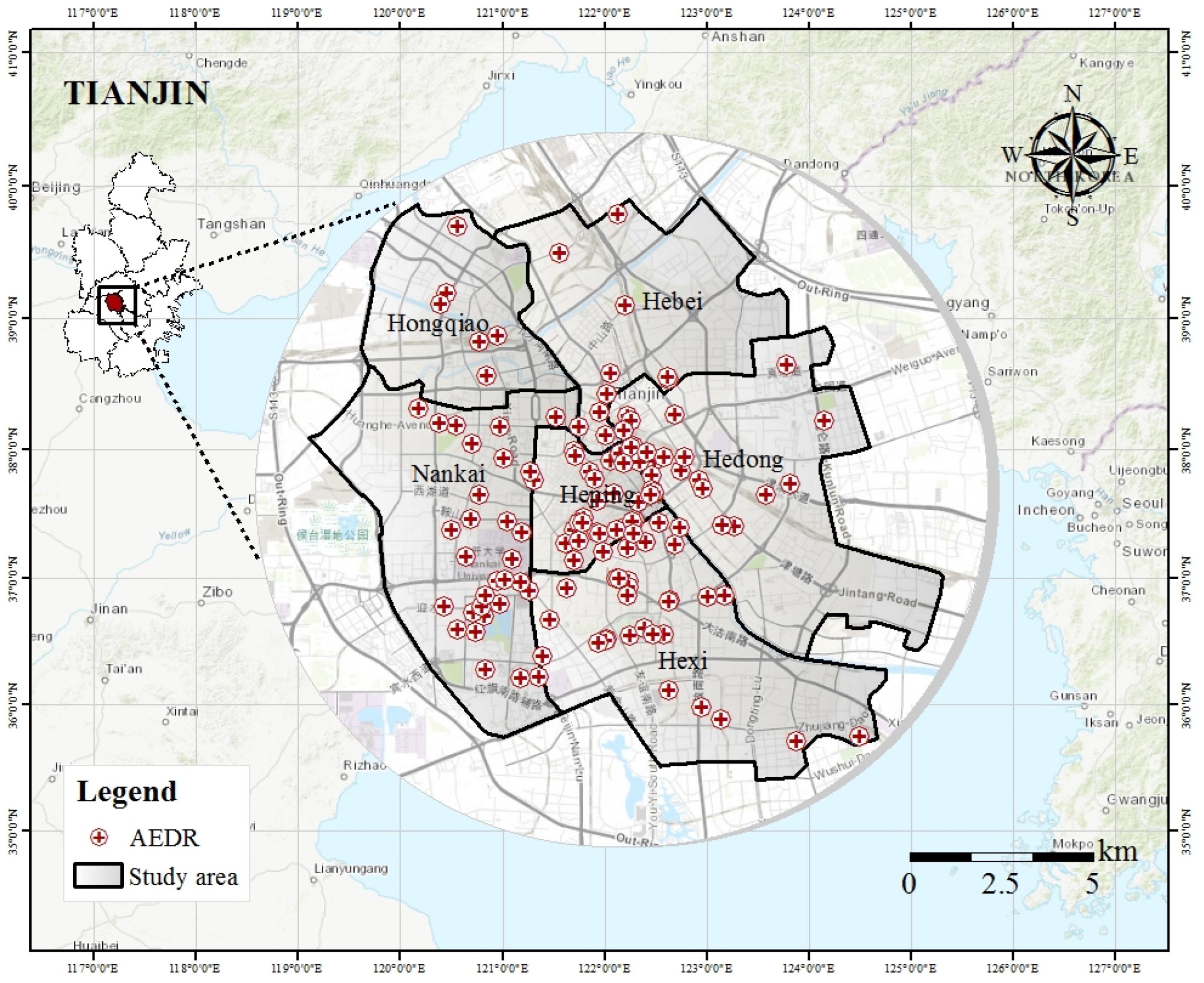
Tianjin (38°34′ N to 40°15′ N, 116°43′ E to 118°04′ E), a coastal megacity in Northern China, is one of the four municipalities directly under the Central Government of China and a pivotal economic hub in the Bohai Rim region [31,32]. The city’s rapid urbanization has intensified challenges in healthcare resource development, particularly in Tianjin Downtown (Figure 1). Spanning 1.73 km2 with a population of 4.0572 million (29.26% of Tianjin’s population within 1.54% of its total land area) [33], this hyper-dense urban core encompasses six administrative districts (Heping, Hedong, Hexi, Nankai, Hebei, and Hongqiao) [31]. We target Tianjin Downtown as the study area for three reasons: (1) The extreme population–land disparity demonstrates significant supply–demand mismatches. (2) Despite 2017 healthcare reforms prioritizing prehospital care optimization [34], Tianjin’s OHCA response system remains underdeveloped, partly driven by inadequate AED placement. (3) The dense built environment and data availability make it an ideal case to model the BE–AEDR nexus in high-density urban cores.
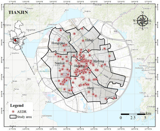
Figure 1.
Location of the study area.
2.2. Framework
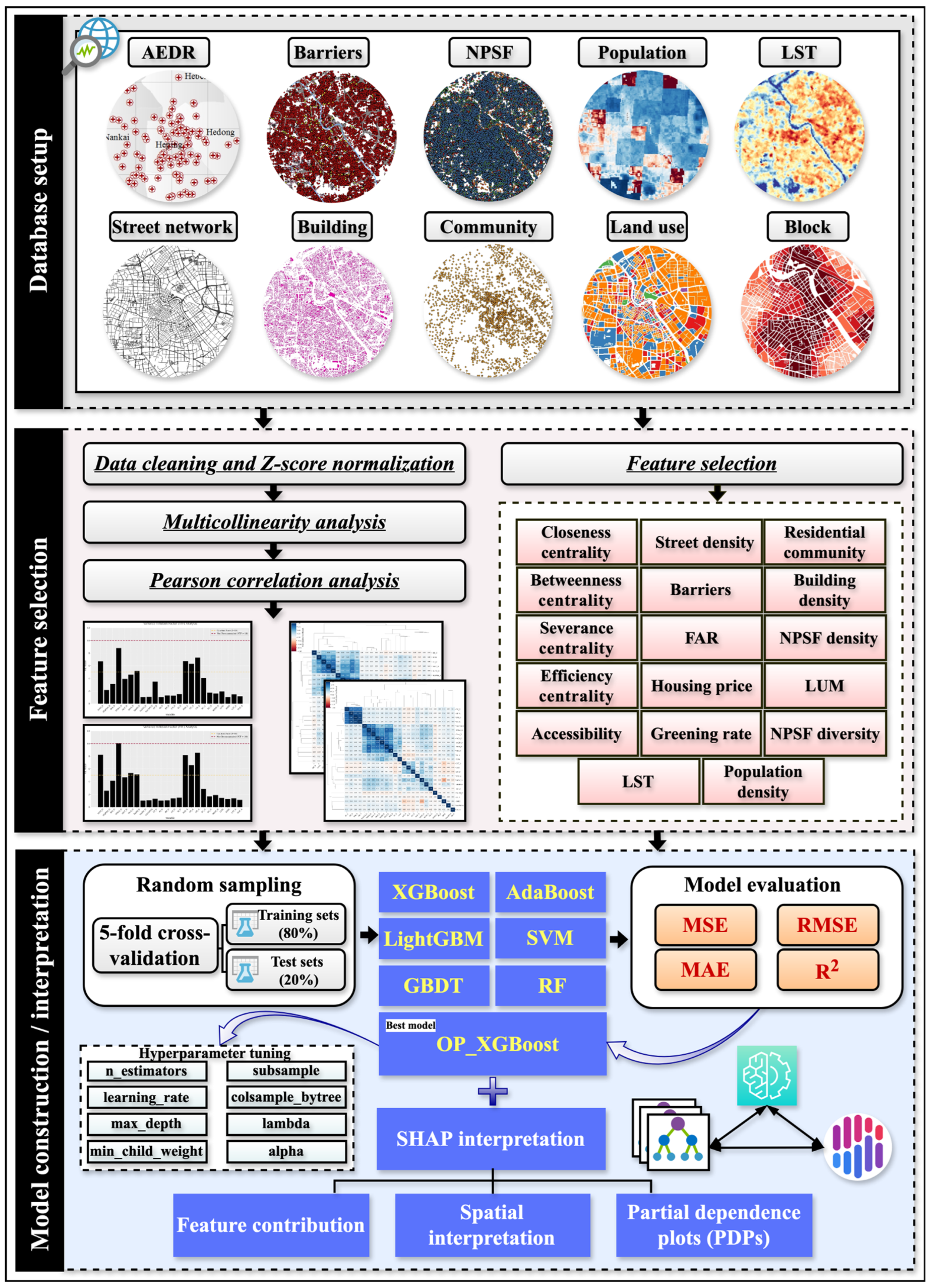
Our study develops an analytical framework to explore the non-linear BE–AEDR spatial nexus in Tianjin Downtown, China (Figure 2). The framework comprises three main phases. (P1) The first phase is related to database setup and preprocessing, including AEDR and BE feature data collection, screening, calculation, and transformation into spatial layers to ensure the elimination of redundancy. (P2) The second phase is related to BE feature selection. Specifically, the potential indicators were identified via extensive literature review, multicollinearity, and Pearson correlation analysis, ensuring the robustness of model input. (P3) The third phase constructs and evaluates the AEDR prediction models. Then, model training, hyper-parameter tuning, and validation were performed step by step. In this study, all procedures run in ArcGIS 10.8 (with a projected coordinate system: WGS_1984_UTM_Zone_50N) and Python 3.9. Finally, we identified limitations of this study and proposed recommendations for AEDR development. To the best of our knowledge, this is the first study to have conducted such a refined analysis of this nature.

Figure 2.
Framework.
2.3. Database Setup
This study utilized three multi-source datasets: AEDR, BE features, and administrative boundaries (Table 1). The first-hand AEDR data, provided by the Tianjin Red Cross Society and supplemented by the geospatial data sourced from the Tianjin EMS and RESCOND WeChat applets, underwent rigorous cleaning of duplicates, errors, and inaccuracies, resulting in 82 valid AEDRs within Tianjin Downtown, which were geocoded and saved into shapefiles. Additionally, the street network data, including crossing and river barriers, were extracted from the OpenStreetMap (OSM) and processed through topological screening: orphan streets were removed, double-line streets were converted into single-line streets, and overlaps were resolved, resulting in 20,708 valid pedestrian-accessible street segments. Furthermore, 3456 residential communities were obtained from Anjuke, China’s largest real estate platform, including attributes such as geographic coordinates, community age, floor area ratio, housing price, greening rate, etc. In parallel, the land-use data were sourced from Gong et al. and classified into residential, commercial, industrial, transportation, and public management types by referring to the Essential Urban Land Use Categories in China (EULUC-China) [35] aligned with the national planning standards (Ministry of Housing and Urban-Rural Development of the People’s Republic of China, 2018; the Ministry of Natural Resources of the People’s Republic of China, 2021). Simultaneously, the buildings, points of interest (POIs), and signage data were crawled via the application program interface (API) provided by AutoNavi one of the largest search engine providers in China. POIs were harmonized with land-use classification to minimize discrepancies (Table A1). Moreover, the land-surface temperature (LST) data were acquired from the USGS Landsat 8 satellite with a spatial resolution of 30 m, while population data were obtained from WorldPop with a spatial resolution of 1 km. The block data were derived from Beiing City Lab (http://www.beijingcitylab.org (accessed on 1 July 2024)), and the national administrative boundaries were obtained from the Chinese Academy of Sciences’ Resource and Environment Science and Data Center.

Table 1.
Data sources.
2.4. Variable Definitions
2.4.1. Dependent Variable: AEDR Intensity Calculation
By referring to previous studies, AEDR density was selected as the dependent variable to capture the spatial heterogeneity attributes. In our paper, Kernel density estimation (KDE) analysis was applied to reflect AEDR intensity in Tianjin Downtown, with 30 m × 30 m cell size and default bandwidth (Table 2) [36]. AEDR intensity (AEDR_D) dependent variable was calculated via KDE analysis, which can be formulated as follows (Equation (1)).
where is the kernel density function of point ; is the distance between point , and the i is the observation point; n is the number of observation points, (i.e., AEDRs) within the radius ; is the kernel function.
Table 2.
Variable definitions.
2.4.2. Independent Variable: BE Feature Calculation
By referring to existing studies, this study delineated BE factors from five dimensions, including comprehensive accessibility, psychological barriers, land use, temperature, and demographics.
(1) Comprehensive accessibility. The comprehensive accessibility was measured by three variables, i.e., street network configuration, service coverage (SC), and street density (ST_D). Street network configuration, a critical determinant of public facility access, was analyzed via the Spatial Network Analysis (sDNA 4.1/https://sdna.cardiff.ac.uk/sdna/ (accessed on 1 May 2024)) technique in the context of space syntax (SS) theory [37,38]. OHCA resuscitation requires AED delivery within 3.5 min [12]. Thus, by referring to Kwon’s formula MD = (f × 2) × f′/2, where f = 1.0 m/s is the maximum walking speed (“Standard for Urban Pedestrian and Bicycle Transport System Planning”) and f′ = 210 s (3.5 min delivery in seconds), the angular choice and integration measures [39], which account for directional influence on route choices, were calculated within a 210 m maximum distance of a bystander. To capture the different dimensions of the street configuration, we computed four indices: closeness (Mean Angular Distance (MAD), network quantity penalized by distance (NQPDA)), betweenness (Betweenness (BtA), Two-phase Betweenness (TPBtA)), severance (Mean Crow Flight (MCF) distance, Diversion Ratio (DivA)), and efficiency (Convex Hull Maximum Radius (HullR), Convex Hull Shape Index (HullSI)) to capture the centrality rate of the street segments [40]. Furthermore, KDE analysis with 30 m × 30 m cell size and default bandwidth was applied to spatially smooth the discrete polylines [41]. SC was evaluated via the Gaussian 2-step Floating Catchment Area (GA2SFCA) method to assess AEDR supply–demand dynamics [42], a widely used approach facility accessibility analysis. Street density (ST_D), a proven EMS accessibility predictor [43], was calculated in ArcGIS through the Intersect tool and length calculation.
(2) Psychological barrier. The psychological barriers, that might delay pedestrian movement, were determined by river density (RI_D), crossing density (CR_D), and signage density (SI_D) [18,44].
(3) Land use. The dimension of land use was assessed by the average floor area ratio (FAR_A) [45], average greening rate (GR_A) [46], residential community count (RC_C), building density (BU_D) [45], nearby public service facility density (NPSF_D) [45], land-use mixture (LUM_SHEI) [47], and nearby public service facility diversity (NPSF_SHDI) [47] as land-use indicators.
(4) Temperature. Existing studies have discovered that BE factors, such as weather conditions, are significantly correlated with EMS response times [45]. The average land surface temperature (LST_A) was used to assess urban heat island effects.
(5) Demographics. Two indicators, average population (POP_A) and average housing price (HP_A), were chosen to reflect demographics and economic activity concentration [17,20].
The KDE cell size of 30 × 30 m was chosen to balance spatial resolution and computational efficiency, consistent with the resolution of ancillary datasets (e.g., LST from Landsat 8) and prior urban spatial analysis literature. All these variables are fundamental BE indicators that reflect the concentration and intensity aspect of residential and commercial endeavors. The driving factor formulas and descriptions are reflected in Table 2, Figure A1 and Figure A2.
2.5. Prediction Model Construction and Performance Evaluation
2.5.1. Data Standardization and Multicollinearity
Ensuring the reliability of the dataset, the z-score standardization method was used, and the missing values were removed. Furthermore, the multicollinearity was assessed via the variance inflation factor (VIF), eliminating the driving factors with VIF > 10 value according to the collinearity verification requirement [48]. The calculation formula is defined as follows (Equation (2)):
where refers to the variance inflation factor of each driving factor and refers to the unadjusted coefficient of determination for regressing the th independent variable on the remaining independent variables [48]. A large VIF value indicates a highly collinear relationship to the other independent variables.
2.5.2. XGBoost and OP_XGBoost Regression Models
XGBoost, an advanced gradient boosting approach proposed by [49], employs classification and regression trees (CARTs) as the base classifier, relying on multiple interconnected decision trees, where the input of the subsequent decision tree is shaped by the prediction and training outcomes of the previous decision tree. Consequently, XGBoost has been widely used through data scientists, providing a parallel tree boosting that handles many ML challenges in a fast and accurate way. In this section, we briefly introduce its mathematics, for additional details; please see the original work on XGBoost model [49]. The XGBoost model can be formulated as follows (Equation (3)):
where denotes the predicted value, corresponds to an independent tree structure with leaf weights, and denotes to the set of all the possible CARTs. The objective function of XGBoost is the sum of the loss function and the regular term, respectively, to control the model accuracy and complexity [50]. The objective function in XGBoost can be formulated as follows (Equation (4)):
where
where l is the convex loss function, which measures the difference between the prediction and target, and denotes a term that penalizes the model complexity. denotes the number of leaves in each tree and denotes the weight associated with and , which indicate the regularization parameters.
In this study, XGBoost model is developed using the sklearn package for jupiter notebook (Python 3.9). To improve the superior performance of the model, we applied the Optuna (OP) hyper-parameter tuning technique combined with a 5-fold cross-validation [51] for dataset partitioning. The RMSE served as the objective function [52]. In general, the model construction process of this study primarily included four steps: dataset partitioning, model selection, model tuning for OP_XGBoost, and model evaluation. The optimal hyper-parameter values and descriptions for the training of the model are shown in Table 3.
Table 3.
Hyper-parameter tunning.
2.5.3. Model Performance Evaluation
To evaluate the model performance, the datasets were randomly split into 80% training and 20% validating sets. Mean Square Error (MSE), Root Mean Squared Error (RMSE), Mean Absolute Error (MAE), and coefficient of determination (R2) were considered four assessment metrics. All the models were resampled 500 times per grid/block unit, and the superior model was selected based on the highest R2 and lowest MSE, RMSE, and MAE. The assessment metrics are defined as formula (Equation (5)):
2.5.4. SHAP Interpretation
To interpret the feature impact on the AEDR intensity, we applied SHAP (SHapley Additive exPlanations) and the partial dependence plots (PDPs). SHAP values quantify the feature importance by computing the weighted contribution of each variable across all possible feature combinations, comparing the model’s prediction with and without the variable [53]. Mathematically, the SHAP values for a feature are calculated as follows (Equation (6)) [54]:
where denotes all the feature set, denotes the feature subset, denotes the factorial of the number of features contained in , and and denote the model trained with and without feature , respectively. The positive, negative, or zero SHAP values indicate features increasing, decreasing, or not affecting the prediction, respectively. For instance, > 0 indicates a positive impact, and < 0 indicates a negative impact [53]. The larger the absolute value of Shapley, the stronger the contribution of the feature [55]. XGBoost and SHAP are often paired in machine learning because they together offer a comprehensive solution for prediction and interpretability. PDPs and locally weighted scatterplot smoothing (LOWESS) trend lines further visualized the complex nonlinear BE–AEDR relationships via local regression smoothing.
3. Results
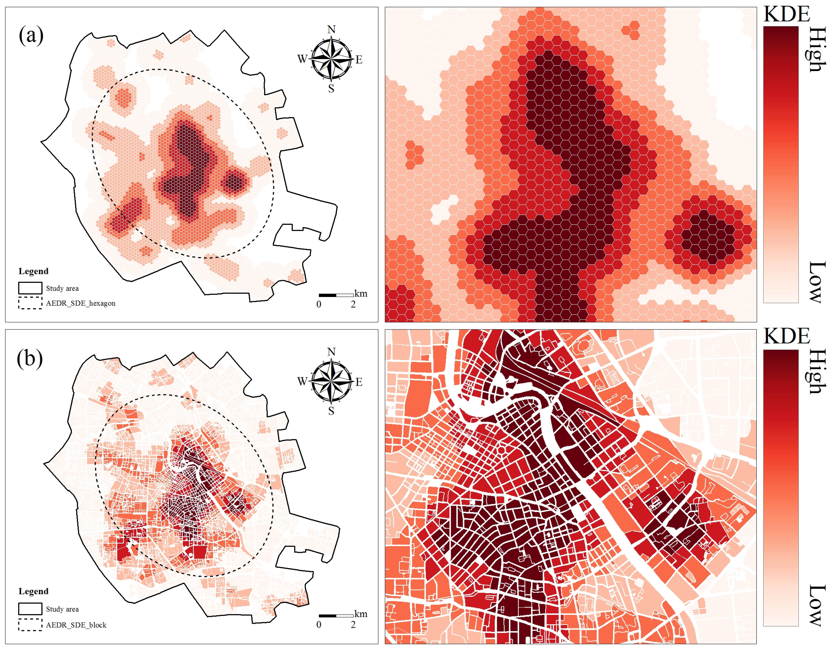
3.1. AEDR Intensity Descriptive Statistics
The AEDR intensity at the grid and block scale in Tianjin Downtown were presented in Figure 3a,b. From the spatial distribution perspective, the results revealed a clear center-edge spatial structure, with a significantly higher intensity in the urban core than in the peripheral areas, particularly with high-intensity clusters in Heping, Nankai, and Hexi districts, and low-intensity clusters in Hongqiao, Hebei, and Hedong districts.
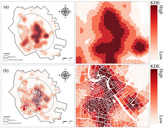
Figure 3.
Intensity trend of AEDRs in Scenario I (a) and Scenario II (b).
The findings demonstrated uneven distribution of AEDRs, pinpointing the hotspot areas with high-density clusters while outlying the peripheral areas with systemic under-provision challenges.
3.2. BE Feature Screening and Correlation Analysis
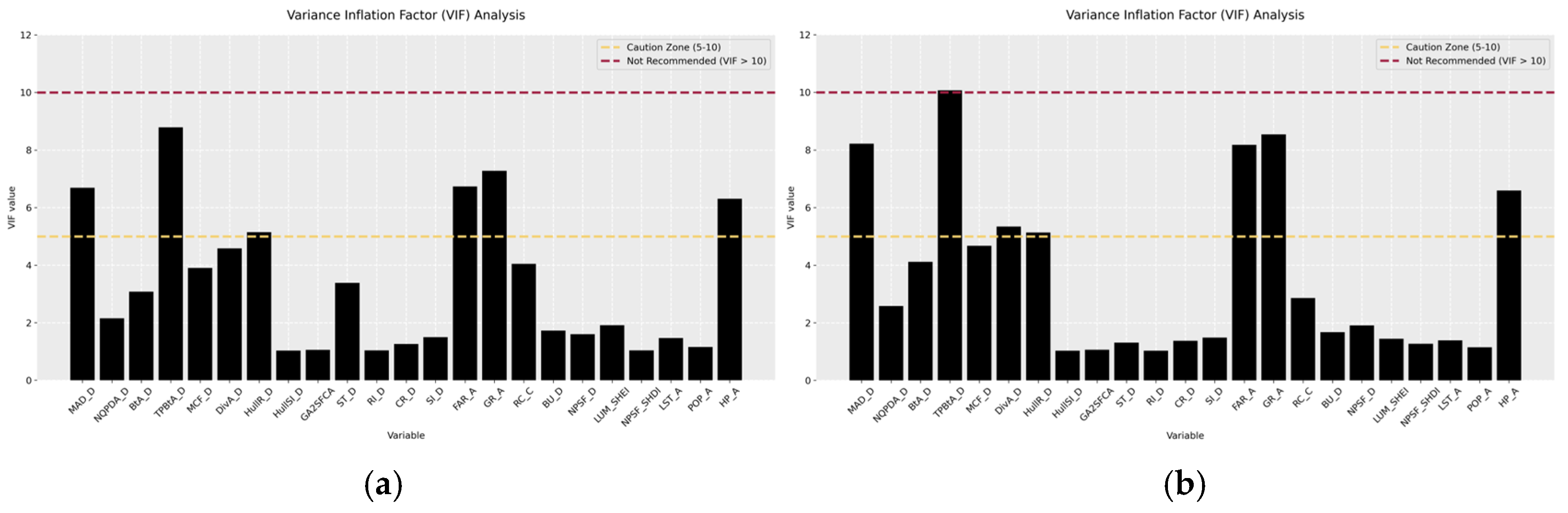
The multicollinearity among 33 independent variables was assessed through VIF, excluding 10 variables with VIF > 10 values, to ensure the model’s reliability. Consequently, 23 variables were retained for analysis (Figure 4a,b).
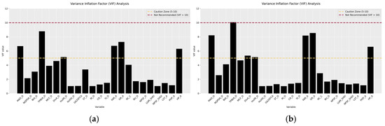
Figure 4.
VIF selected features in Scenario I (a) and Scenario II (b).
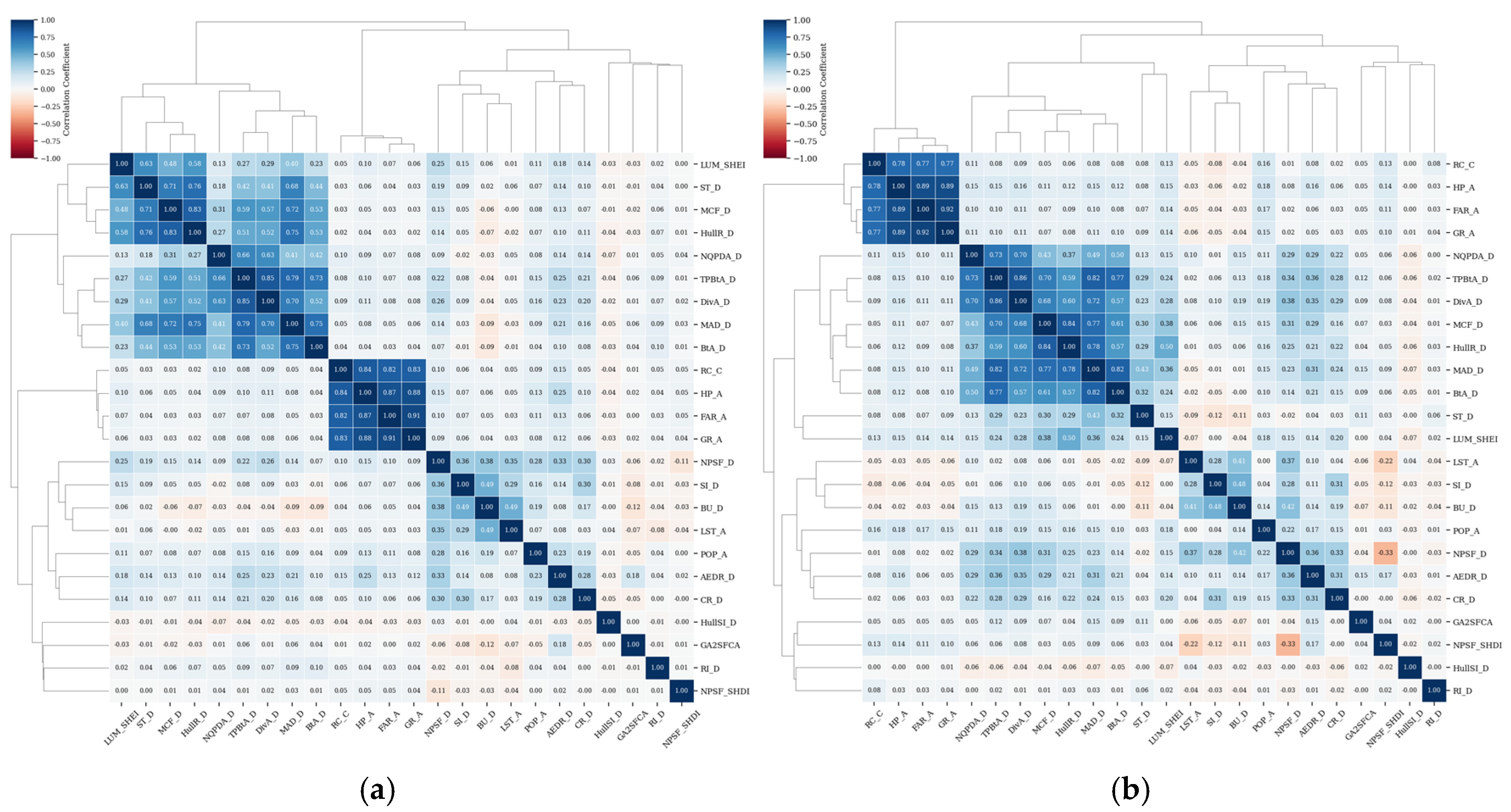
Upon the Pearson correlation coefficient heatmap observation (Figure 5a,b), it is evident that there exists a significant correlation among multiple features. Strong positive correlations were observed between AEDR_D and FAR_A (r = 0.91 and r = 0.92 in SI and SII, respectively), HP_A (r = 0.87 and r = 0.89 in SI and SII, respectively), and TPBtA_D (r = 0.85 and r = 0.86 in SI and SII, respectively), suggesting AEDR concentration in high-density urban areas and transportation hubs. In contrast, several variables display notably weak correlations with AEDR_D, such as GA2SFCA (r = −0.01 and r = 0.02 in SI and SII, respectively), CR_D (r = −0.05 and r = −0.06 in SI and SII, respectively) and HullSI_D (r = 0.00 and r = −0.00 in SI and SII, respectively), reflecting potential gaps and less-served areas. Pearson correlation and VIF values of all the variables are shown in Table A2.

Figure 5.
Correlation matrix among the selected features in Scenario I (a) and Scenario II (b).
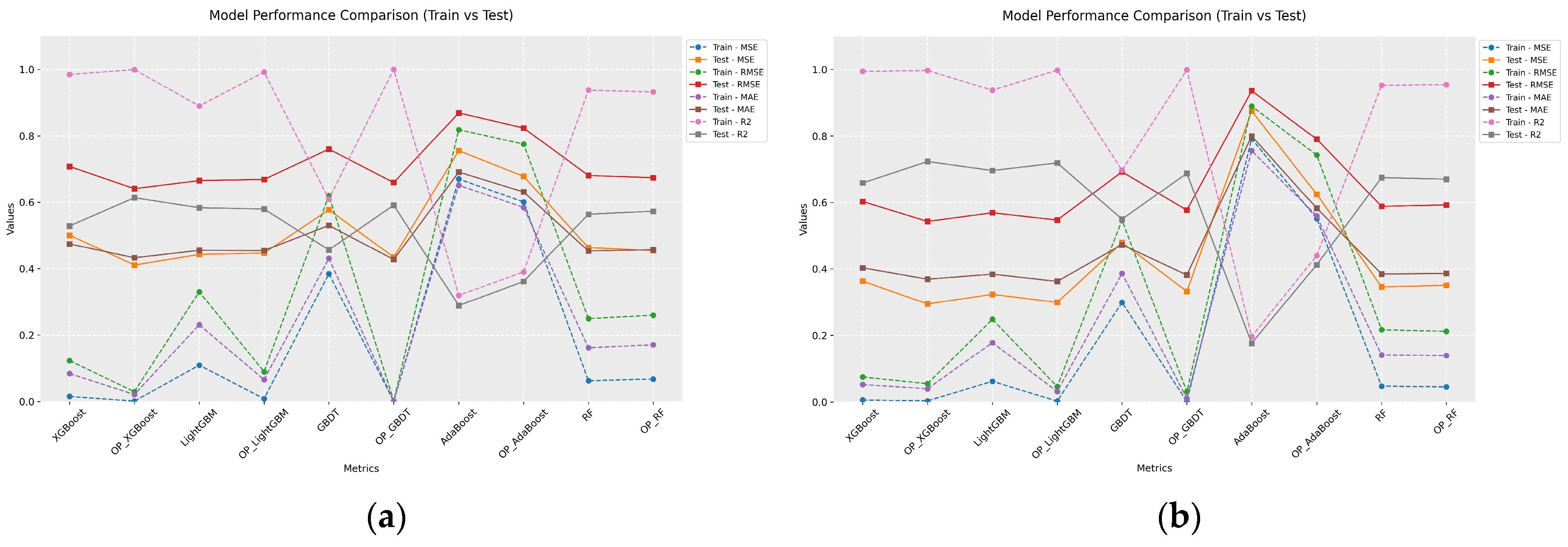
3.3. Performance Evaluation of the Prediction Models
Figure 6a,b shows the scatter plots of the models’ performance predicted on the train and test sets at the grid (SI) and block scales (SII). The performance results of the 10 models (XGBoost, OP_XGBoost, LightGBM, OP_LightGBM, GBDT, OP_GBDT, AdaBoost, OP_ AdaBoost, RF, OP_RF) were evaluated via MSE, RMSE, MAE, and R2 (Table A3 and Table A4).
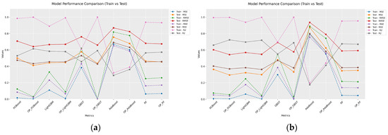
Figure 6.
Performance of the models in Scenario I (a) and Scenario II (b).
In SI, OP_XGBoost achieved the highest R2 = 0.61 and the lowest RMSE = 0.64, while MSE = 0.41 and MAE = 0.43 outperform other models, particularly XGBoost (R2 = 0.53, RMSE = 0.71, MSE = 0.50, MAE = 0.47), LightGBM (R2 = 0.58, RMSE = 0.67, MSE = 0.44, MAE = 0.46), OP_LightGBM (R2 = 0.58, RMSE = 0.67, MSE = 0.45, MAE = 0.45), GBDT (R2 = 0.46, RMSE = 0.76, MSE = 0.58, MAE = 0.53), OP_GBDT (R2 = 0.59, RMSE = 0.66, MSE = 0.43, MAE = 0.43), AdaBoost (R2 = 0.23, RMSE = 0.87, MSE = 0.76, MAE = 0.70), OP_AdaBoost (R2 = 0.36, RMSE = 0.82, MSE = 0.68, MAE = 0.63), RF (R2 = 0.56, RMSE = 0.68, MSE = 0.46, MAE = 0.45), and OP_RF (R2 = 0.57, RMSE = 0.67, MSE = 0.45, MAE = 0.46).
In SII, the OP_XGBOOST model demonstrated even superior performance, achieving the highest R2 = 0.72 and the lowest RMSE = 0.54, MSE = 0.30, and MAE = 0.37, which was significantly better than the XGBoost (R2 = 0.66, RMSE = 0.60, MSE = 0.36, MAE = 0.40), LightGBM (R2 = 0.70, RMSE = 0.57, MSE = 0.32, MAE = 0.38), OP_LightGBM (R2 = 0.71, RMSE = 0.55, MSE = 0.30, MAE = 0.36), GBDT (R2 = 0.55, RMSE = 0.70, MSE = 0.48, MAE = 0.47), OP_ GBDT (R2 = 0.69, RMSE = 0.58, MSE = 0.33, MAE = 0.38), AdaBoost (R2 = 0.18, RMSE = 0.94, MSE = 0.88, MAE = 0.80), OP_ AdaBoost (R2 = 0.41, RMSE = 0.79, MSE = 0.63, MAE = 0.58), RF (R2 = 0.68, RMSE = 0.59, MSE = 0.35, MAE = 0.39), and OP_ RF (R2 = 0.67, RMSE = 0.59, MSE = 0.35, MAE = 0.39).
The notable improvements in OP_XGBoost at the block scale affirm its theoretical and practical relevance, emphasizing the adoption of OP_XGBoost at the block scale as the superior analytical approach for further spatial analysis.
3.4. Results of Modelling Interpretation
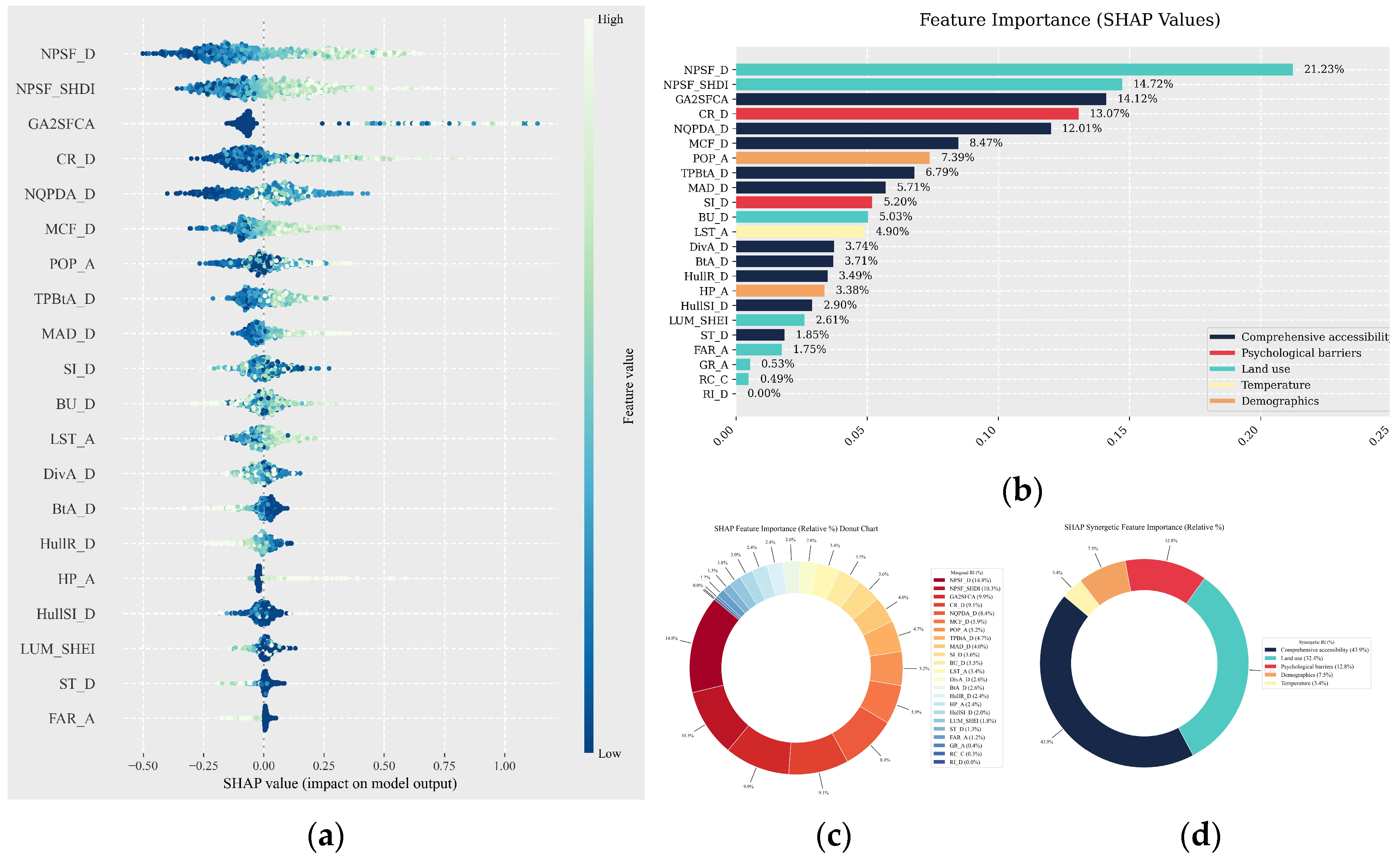
3.4.1. Feature Importance Disparities
Figure 7a–d and Figure 8a–d showed the results of the absolute importance (AI), relative importance (RI), and rankings of independent variables in Tianjin Downtown. Feature importance (SHAP values) refers to the absolute importance (AI), inherently accounting for interactions. Both the absolute importance (AI) and relative importance (RI) were analyzed in the context of marginal and synergetic contributions. The marginal contribution denotes the isolated impact of a single feature on the model’s output. The synergetic contribution denotes the hierarchical groupings of features to assess the combined impact on the model’s output. The SHAP summary plot (Figure 7a and Figure 8a) and BE-AI (Figure 7b and Figure 8b) enabled the determination of the positive and negative contributions of feature importance. The horizontal coordinate represented the SHAP value, with the color of each sample point indicating the height of the sample value; lower sample values corresponded to higher SHAP values, indicating a negative contribution, and vice versa for positive contributions.
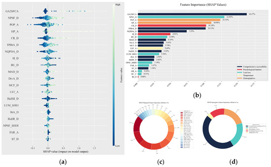
Figure 7.
SHAP mean values (a), AI (b), marginal RI (c) and synergetic RI (d) in Scenario I.
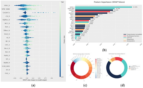
Figure 8.
SHAP mean values (a), AI (b), marginal RI (c) and synergetic RI (d) in Scenario II.
In terms of the marginal contribution (Figure 7c and Figure 8c), the BE-RI displayed a continuously varying contribution trend across the two units. The top 10 variables in SI included GA2SFCA, NPSF_D, POP_A, HP_A, CR_D, TPBtA_D, NQPDA_D, SI_D, BU_D, and MAD_D, whereas other variables were negatively correlated, with AEDR intensity demonstrating lower RI effects. Consequently, the top 10 variables in SI included NPSF_D, NPSF_SHDI, GA2SFCA, CR_D, NQPDA_D, MCF_D, POP_A, TPBtA_D, MAD_D, and SI_D. The RI of the GA2SFCA showed a continuously decreasing contribution rate of 13.2% and 9.7% in the SI and SII, respectively, appearing to hold predictive importance, and ranking first in the grid model and third in the block model. Conversely, NPSF_D demonstrated a progressive increase in importance, ranking second in the grid model and first in the block model, as well as showing a continuously increasing contribution rate of 10.5% and 14.8% in the SI and SII, respectively.
In terms of the synergistic contribution (Figure 7d and Figure 8d), the BE-RI displayed a relatively congruent contribution with a slight difference. The synergistic contribution rate of the comprehensive accessibility indicators stood at 45.1% and 43.9% in the SI and SII models, respectively. In contrast, the land-use indicators showed a higher contribution, standing at 20.7% and 32.4% in the SI and SII models, respectively, whereas the demographic indicators, with 19.0% and 7.5% in the SI and SII, showed adaptivity lower contributions. Additionally, the psychological barrier indicators demonstrated 12.3% and 12.8% and the land surface temperature indicators 3% and 3.4% in the SI and SII models, respectively. The findings revealed that comprehensive accessibility and land use play a significant role, ranking first and second in both SI and SII, underscoring the significance of the top BE features in influencing AEDR.
The findings provide two insights. First, BE features are overlooked in AEDR-related studies. In contrast, the impact of a single BE feature on AEDR varies, with some features demonstrating significant influence, while others show negative influence, highlighting the heterogeneous nature of the BE-AEDR nexus. Second, the results suggest that the influence of the BE is highly interactive with proximity to the AEDR, with the maximum influence exerted within bock pattern, which not only underscores the reason for the superior model performance but also advocates for urban designers and planners to prioritize this block pattern to maximize the effectiveness of BE-related interventions. Our findings affirm the multi-scale nature of urban environments, where certain features dominate at finer resolutions while others emerge at broader scales. This underscores the need to consider multiple spatial units to capture the full spectrum of the BE-AEDR nexus, ensuring a more robust and comprehensive urban health infrastructure planning.
3.4.2. Spatial Contribution of Independent Variables
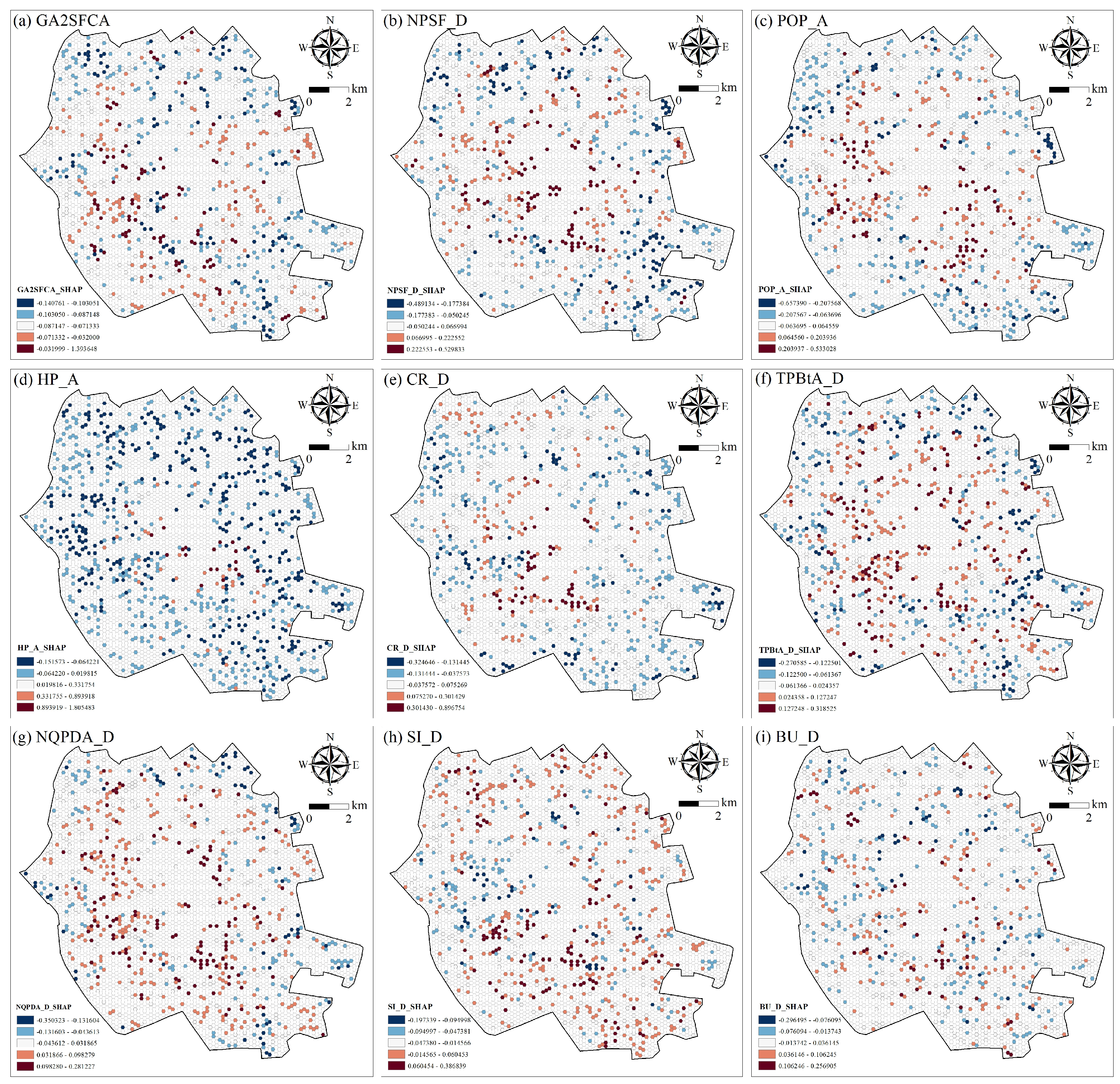
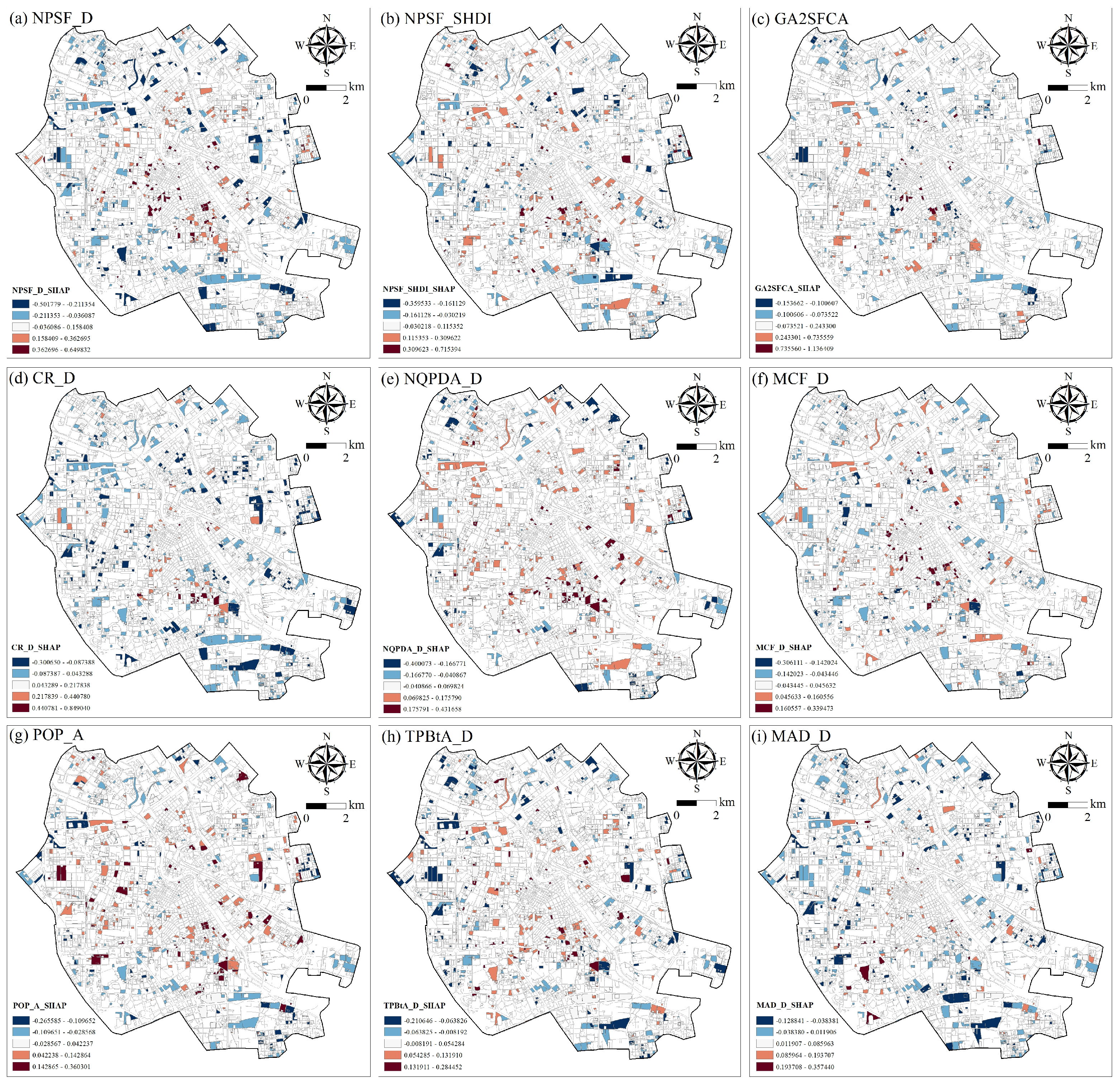
The study calculated and analyzed the average SHAP values for each grid cell and block in Tianjin Downtown. Figure 9 and Figure 10 illustrate the spatial distribution of SHAP values for the primary nine key BE features, highlighting the nuances of spatial patterns and reflecting spatial heterogeneity and spatial consistency trends, ultimately enhancing the underserved peripheral zones.
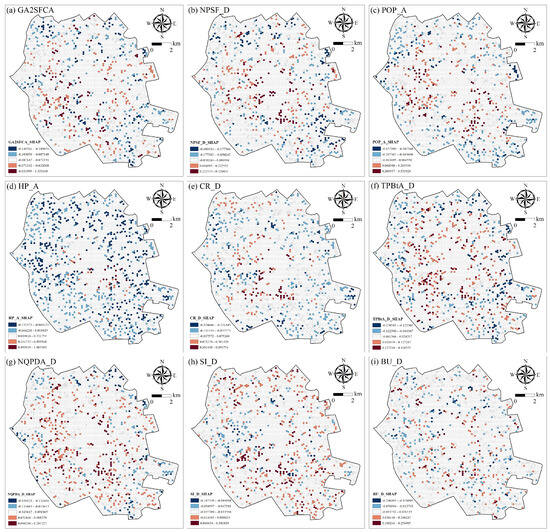
Figure 9.
Grid patterns of SHAP values in a sample experiment with 20% sampling ratio.
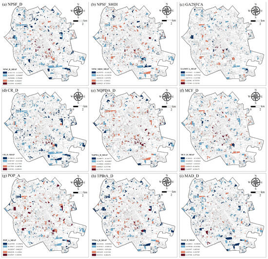
Figure 10.
Block patterns of SHAP values in a sample experiment with a 20% sampling ratio.
The spatial performance of key variables revealed spatial heterogeneity and spatial consistency trends. This phenomenon highlighted the influence of spatial resolution on the interpretation of SHAP values.
At the grid scale, GA2SFCA showed strong positive contributions in the southern and eastern areas, reflecting high AED accessibility in these regions. Northern grids exhibited predominantly negative SHAP values, indicating significant gaps in AED accessibility. At the block scale, positive contributions were observed in eastern areas, suggesting finer localized accessibility. However, northern and western blocks showed more fragmented negative values. While both scales identified northern areas with limited accessibility, the block scale reveals finer spatial heterogeneity, uncovering intra-grid disparities. NPSF_D and NPSF_SHDI displayed a mixed pattern, with negative SHAP values concentrated in the urban core and western patterns, suggesting facility saturation, and positive contributions were dispersed across central, northern, and eastern patterns. Positive SHAP values emerged in southern blocks, while negative values clustered in the central areas, reinforcing the grid-level findings but with more pronounced variations across adjacent blocks. POP_A showed contrasting patterns, with positive contributions in southern and eastern grids and negative values in the north. Population influence was more spatially fragmented at the block scale, with positive values in eastern areas, while the grid scale revealed broader population trends. This phenomenon suggests that population impact on AEDR might operate at varying spatial resolutions. HP_A demonstrated a minor positive contribution across the southwest grids. The peripheral grids reflected localized negative SHAP values. The grid scale captured macro-level trends in housing price influence and smoothed the local discrepancies, reinforcing the pervasive impact of socio-economic conditions on AEDR. CR_D predominantly displayed negative contributions across the southwestern grids, implying that high crossing density hinders AED accessibility. The block scale revealed smaller patches of positive contributions in eastern and southern areas, with negative values concentrated in the north. High positive contributions of TPBtA_Ds appeared in central grids, suggesting that network connectivity enhances AED accessibility. Block scale analysis reflected similar trends, with certain blocks showing negative contributions. TPBtA_D’s positive influence was consistent across both scales, highlighting network connectivity benefits. NQPDA_D showed positive SHAP values clustered in eastern, southern, and western grids, reflecting highly efficient road networks. Fragmented grids in the peripheral areas exhibited negative contributions. Similar patterns emerged at the block scale, while MAD_D and MCF_D showed fragmented contributions with emphasized micro-level accessibility challenges. SI_D demonstrated positive contributions dominating outer grids, while negative values were concentrated in the eastern areas. BU_D exhibited mixed contributions across central grids, with scattered positive values most in eastern and southern grids, highlighting potential redevelopment opportunities.
In conclusion, spatial SHAP uncovered pattern dependency, emphasizing the spatial heterogeneity and spatial consistency trends, showing how the variable contributions vary across space, while others exhibit stability. SHAP spatial maps identified underserved grids and blocks, informing targeted interventions to address AEDR development challenges.
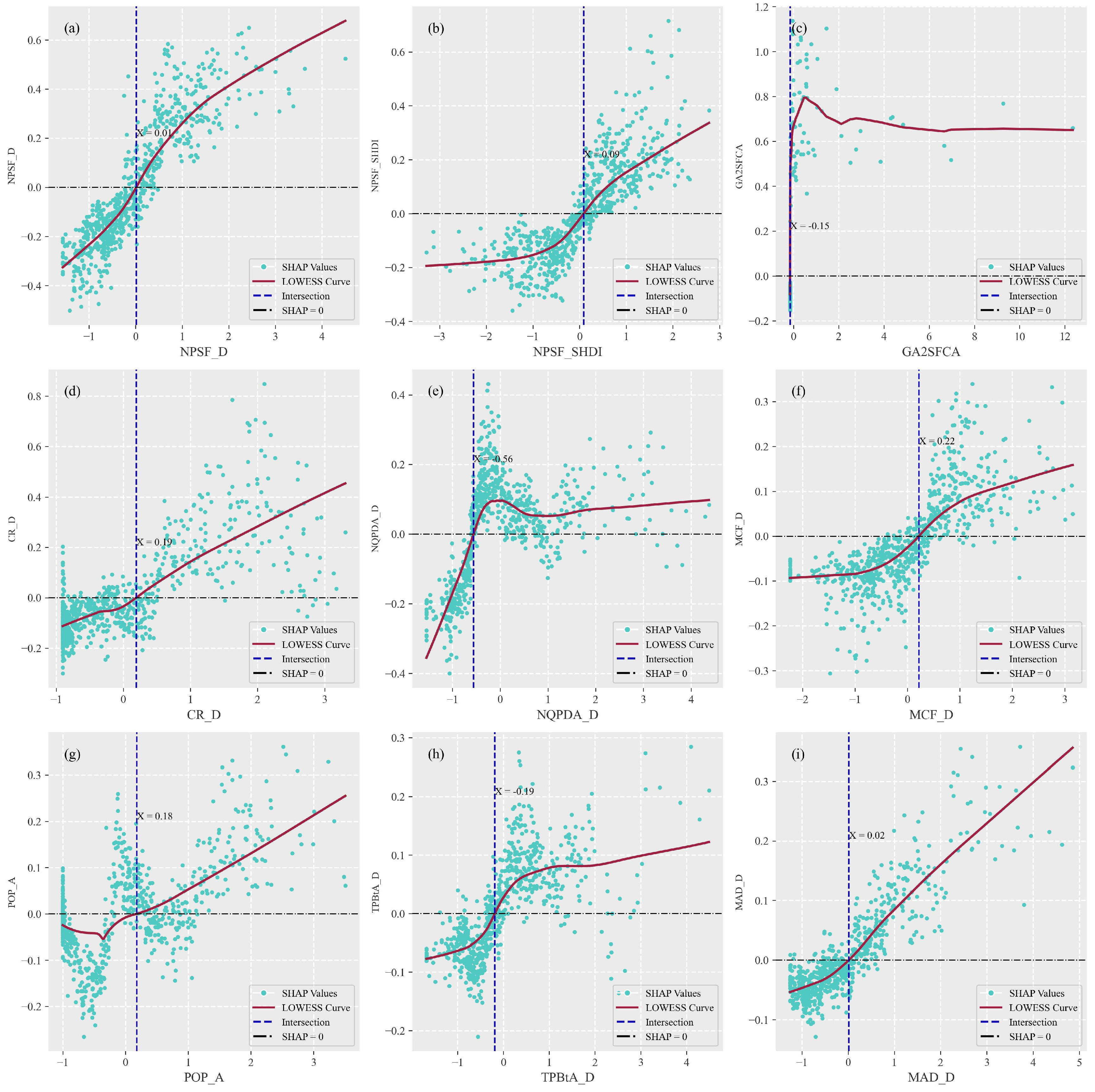
3.4.3. Non-Linear Impact of BE Features on AEDR Intensity
To capture the inherent complexities of the feature dependence and non-linear effects of the primary nine BE features, the SHAP scatter plot and PDPs were utilized. The scatter plots indicated the degree of positive/negative features’ influence on the AEDR intensity, while the fitted LOWESS curve revealed the threshold effects across grid and block patterns, as shown in Figure 11 and Figure 12.
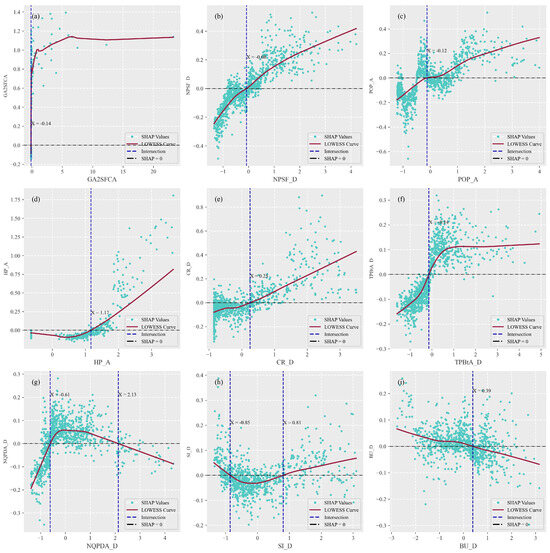
Figure 11.
Non-Linear impact of BE features on AEDR intensity in Scenario I.
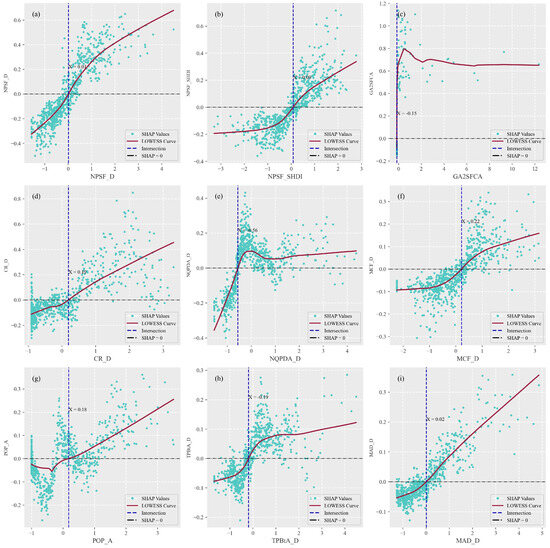
Figure 12.
Non-Linear impact of BE features on AEDR intensity in Scenario II.
For comprehensive accessibility, the GA2SFCA plots showed positive effects beyond the feature values of x ≈ −0.14 (SI) and −0.15 (SII). Further, the values plateau, indicating a relatively balanced effect on AEDR intensity. The TPBtA_D exhibited a critical threshold effect at x ≈ −0.14 (SI) and x ≈ −0.19 (SII), shifting from negative to positive, suggesting prioritized AEDR placement in well-connected and accessible areas. The NQPDA_D displayed an inverse U-shaped correlation with AEDR, indicating a negative–positive–negative pattern peaking around from x ≈ −0.61 to x ≈ 2.13 (SI), contributing negatively at both ends. While SII showed a negative–positive effect with intersection x ≈ −0.56, characterized by stabilization thereafter. The MAD_D and MCF_D demonstrated positive impact at the threshold x ≈ 0.02 (SII) and x ≈ 0.22 (SII), respectively. The positive values indicated well-connected and accessible areas, while negative values indicated lower accessibility, emphasizing the significance of enhancing AEDR accessibility in underserved areas. Physiological barrier analysis revealed the CR_D’s slight positive contribution, becoming more pronounced beyond x ≈ 0.25 (SI) and x ≈ 0.19 (SII), while SI_D exhibited a U-shaped effect, shifting from negative to positive, with the lowest threshold effect beyond x ≈ −0.85 (SI) and the highest threshold around x ≈ 0.81 (SI). This reflected the complex navigation dynamics, where sparsely distributed crossings and signages act as barriers, while well-planned and clustered signages improve AED response. Land-use dynamics showed the NPSF_D shifting from negative to a positive effect, with a critical threshold effect beyond x ≈ −0.08 (SI) and x ≈ 0.01 (SII), indicating sensitivity to NPSF density. The BU_D showed moderate positive trends below x ≈ 0.39 (SI) then decreased gradually, indicating negative impact, possibly due to sparse building distribution, while NPSF_SHDI shifted from neutral to positive nonlinear contribution as feature values increased. Initially, the effect became evident at the x ≈ 0.09 (SII) threshold, suggesting areas with lower diversity exhibit no impact, while higher diversity exhibits positive impact, affirming the contributions of the mixed-use areas to pre-EMS service coverage. Demographic factors demonstrated HP_A’s strong non-linear correlation as the housing price increased, with the threshold beyond x ≈ 1.17 (SI), characterized by better infrastructure resources. In the areas with lower housing prices, the effect was balanced and not significant, reflecting that less developed areas were underserved. POP_A showed slightly distinct trends: a negative–positive shift at x ≈ −0.12 (SI) and a V-shaped positive–negative–positive shift at x ≈ 0.18 (SII).
In general, PDPs with the threshold effect were excellent in detecting the overall non-linear BE–AEDR nexus dynamics, enhancing the model accuracy and interpretability.
4. Discussion
The integration of BE considerations into AEDR planning is pivotal for enhancing pre-EMS accessibility in urban settings. This study bridges methodological and theoretical gaps by employing explainable ML models to unravel the BE–AEDR nexus, offering actionable insights for sustainable urban health planning. AEDRs have relatively dispersed geographical locations in Tianjin because they have usually been rigorously screened and jointly determined by investors, governors, and experts. Traditional AED planning studies have largely relied on linear regression or heuristic approaches, which oversimplify the intricate interactions between urban features and AEDR. This study advances the field by integrating explainable ML algorithms, notably the OP_XGBoost model optimized with SHAP. The OP_XGBoost outperformed benchmark models (e.g., XGBoost, RF, etc.) across both grid (R2 = 0.61) and block (R2 = 0.72) scales, demonstrating superior predictive accuracy and robustness. Unlike “black-box” models, the SHAP framework provided granular interpretability, revealing how BE features influence AEDR intensity. This methodological shift underscores the value of ML in capturing urban complexity while maintaining transparency, a critical requirement for policymakers prioritizing evidence-based decisions. Future studies could extend this approach to other cities, validating its generalizability across diverse urban morphologies. Below, we contextualize the key findings, emphasizing their academic significance and practical implications.
4.1. Bridging Accessibility and Land-Use Efficiency
The SHAP analysis highlighted pronounced disparities in feature importance across spatial resolutions. At the grid scale, comprehensive accessibility metrics like GA2SFCA dominated, contributing 13.2% to AEDR intensity, while at the block scale, nearby public service facility density (NPSF_D, 14.8%) emerged as the most influential. This divergence underscores the multi-scale nature of BE impacts: macro-scale accessibility governs broad AED placement, whereas micro-scale land-use efficiency (e.g., clustered services) becomes critical at finer resolutions. Synergistically, comprehensive accessibility and land-use indicators collectively contributed 45.1% and 43.9% to model predictions, emphasizing their centrality in AEDR planning. Eastern and southern zones exhibited strong positive contributions at the grid scale, reflecting robust AED coverage, whereas northern and western areas showed fragmented accessibility gaps, particularly at the block scale. Notably, the urban core and western zones displayed facility saturation and demonstrated unmet demand. Such insights necessitate tailored interventions, such as boosting AED deployment while targeting micro-level inefficiencies in underserved zones, like northern and western zones, to dramatically improve OHCA outcomes.
4.2. Spatial Resolution and Pattern Dependency as Game-Changers: Block-Level Granularity Redefines Urban AED Planning
The study’s most striking revelation was the superior predictive performance of block-level models over grid-based ones. This aligns with urban design principles, where blocks, as functional units of pedestrian movement, better encapsulate localized BE interactions. The revealed spatial heterogeneity and consistency gaps by SHAP spatial maps advocate for multi-scale planning frameworks, where block-level granularity complements city-wide grids to address micro-level disparities.
4.3. Nonlinear Dynamics: Threshold Effects and Policy Levers
The non-linear association between the BE and AEDR could provide input for creating bystander-friendly AEDRs in high-density cities. The relationships between the built environment attributes and AEDR intensity exhibit non-linearity. The non-linear patterns offer valuable geographical insights that facilitate a deeper understanding of AEDRs within varying environmental contexts. These patterns help to clarify how different environmental factors foster specific infrastructure development in non-linear ways, ensuring resources align with the dynamic urban rhythms.
Our findings provided valuable policy implications for urban planners and policymakers to improve future AED deployment. (1) First, since AEDR intensity was influenced by various factors, the contribution analysis prioritized the importance of the comprehensive accessibility feature for future AED placement. We note that the city center does not provide a suitable walking environment. Targeting areas with low AED accessibility, accounting for groupings of the features, can help urban planners to draw more comprehensive policies, providing diverse short-distance travel and ensuring a smooth travel system for residents’ emergency requirements. (2) Second, geospatial analyses at the block scale could be beneficial for stakeholders to locate AEDs in underserved areas, reducing spatial mismatches between supply and demand. (3) Third, BE features exhibit non-linear associations with AEDR intensity, with variable-specific positive and negative thresholds. Failure to account for non-linearity may lead to underestimation of the impacts of certain variables. It is recommended that urban planners identify critical BE features to enhance AEDR usage effectively. In summary, decision-makers should consider the BE non-linear effects when formulating urban planning strategies. Understanding these effects empowers urban planners and policymakers to make more informed decisions regarding city design and planning.
5. Conclusions
AEDs are critical interventions in cardiac arrest treatment, improving OHCA survival outcomes by up to 70%. Therefore, this study established an interpretable ML-based framework and used novel datasets to uncover the complex interplay of the BE-AEDR in Tianjin Downtown.
The principal conclusions are as follows: (1) Marginally, the AEDR intensity was greatly influenced by the GA2SFCA at grid scale and NPSF_D at block scale, as well as synergistically by the comprehensive accessibility at both scales. Furthermore, the block pattern demonstrated superior performance in testing model; (2) Pattern-dependent effects existed between BE–AEDR factors, while SHAP values vary across specific patterns, emphasizing localized spatial heterogeneity and spatial consistency trends; (3) The BE-AEDR non-linear relationships were uncovered, demonstrating distinct positive and negative correlations with the threshold effects. Overall, the interpretable ML-based approach in this study demonstrated excellent predictive outcomes by setting health at the heart of the urban development approach.
Despite the robust analytical framework, this study has several limitations. First, the unavailability of OHCA incident data, as the incident spatiotemporal variations may skew AED demand predictions. Second, the analysis prioritizes pedestrian street networks, neglecting the spatiotemporal dynamics of drivers and cyclists, whose behavioral movement fluctuates, such as route preferences and speed variations. Third, the focus on the grid and block spatial units fails to address urban–rural heterogeneities in the BE–AEDR context, which could introduce variability not captured in the current model. Addressing these gaps requires multi-modal mobility data and optimized ML models, offering a more comprehensive view of urban planning and emergency preparedness, ensuring alignment with real-world needs.
Overall, this study provided scientific support for policymakers and urban planners to prioritize life-saving resource development via capturing the BE–AEDR nexus. The framework is generalizable and can be applied to settings with the same geographical features, ensuring both methodological rigor and practical applicability.
Author Contributions
Conceptualization, Sara Grigoryan; methodology, Sara Grigoryan; software, Sara Grigoryan; validation, Sara Grigoryan; formal analysis Sara Grigoryan; data curation, Sara Grigoryan; writing—original draft preparation, Sara Grigoryan; writing—review and editing, Sara Grigoryan and Nadeem Ullah; visualization, Sara Grigoryan; supervision, Yike Hu. All authors have read and agreed to the published version of the manuscript.
Funding
This research received no external funding.
Data Availability Statement
Data will be made available on request.
Conflicts of Interest
The authors declare no conflicts of interest.
Appendix A
Appendix A.1
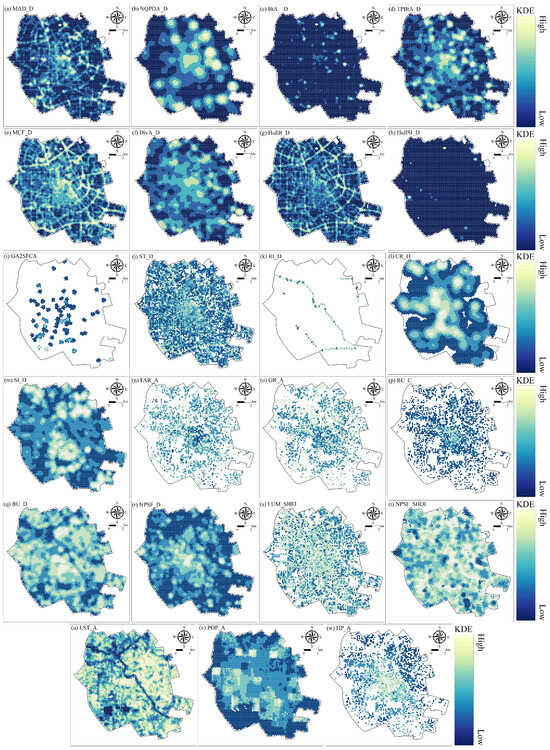
Figure A1.
Spatial distribution of the selected BE variables in Scenario I.
Figure A1.
Spatial distribution of the selected BE variables in Scenario I.
Appendix A.2
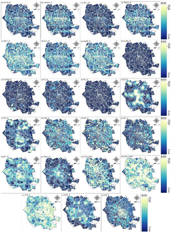
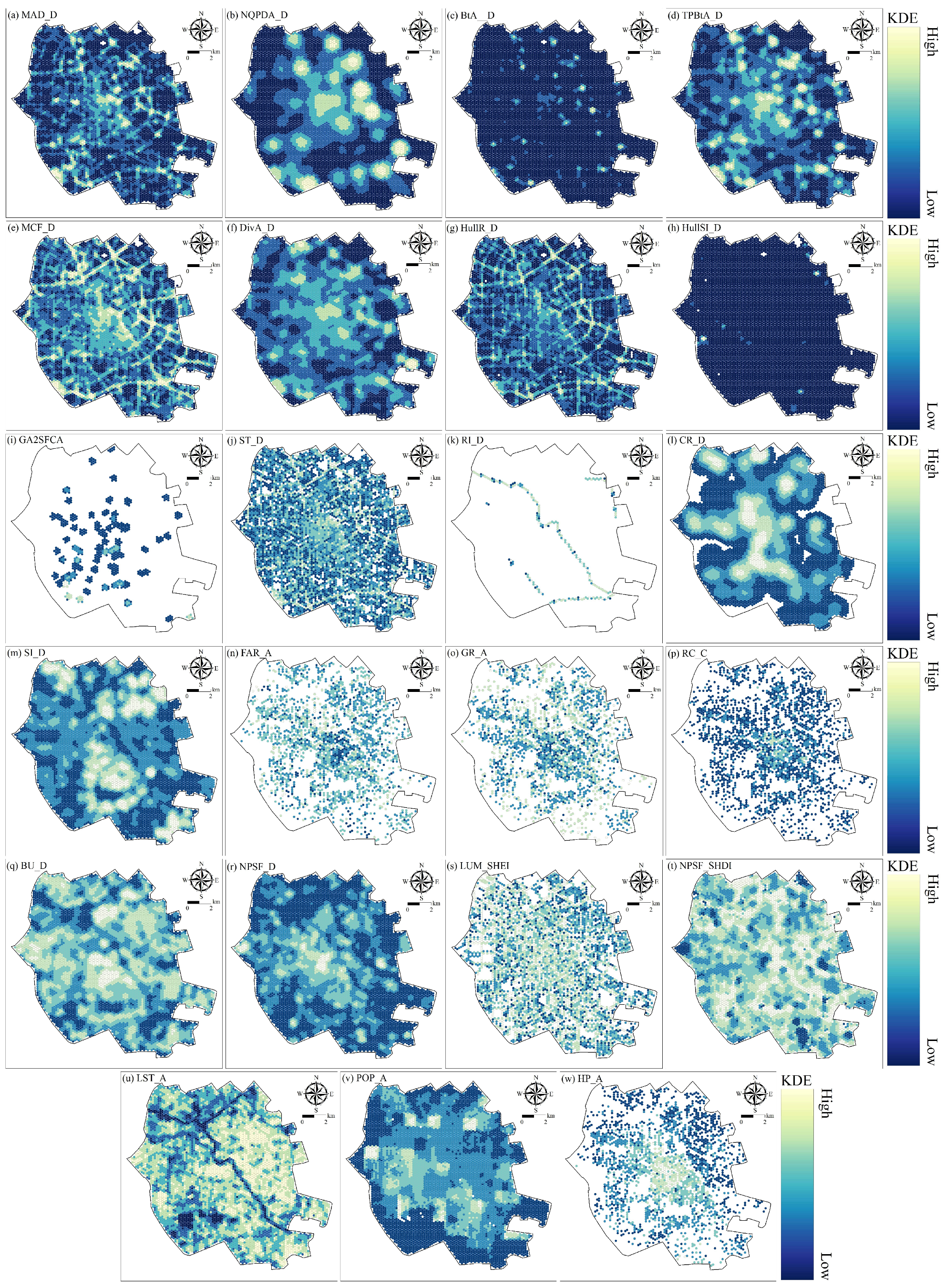
Figure A2.
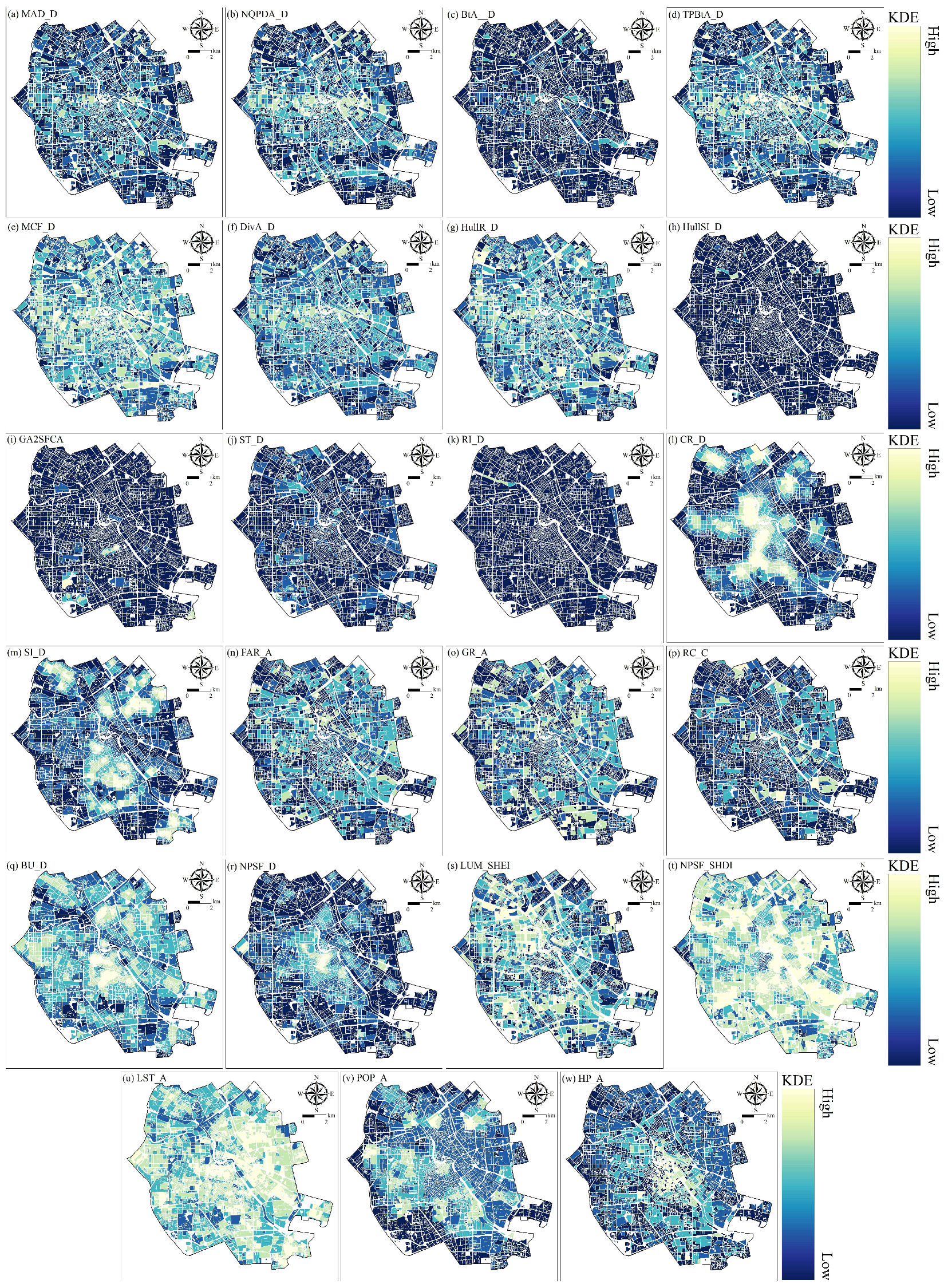
Spatial distribution of the selected BE variables in Scenario II.
Figure A2.
Spatial distribution of the selected BE variables in Scenario II.
Appendix B
Appendix B.1
Table A1.
POI classification.
Table A1.
POI classification.
| Level I | Level II | Number | Percentage (%) |
|---|---|---|---|
| Residential | Residences (community) | 3456 | 3.02% |
| Commercial | Business and finance (company, bank, ATM, security office, etc.), commerce (convenience store, supermarket, shopping mall, store, shopping-related place, etc.), and catering (catering venue, restaurant, fast food venue, tea-coffee house, etc.) | 76,551 | 66.81% |
| Industrial | Industry (factory) | 142 | 0.12% |
| Transportation | Transportation facilities (railway station, subway station, bus station, taxi station, port, parking lot, etc.) | 9500 | 8.29% |
| Public management and service | Administration (government institution, social organization, foreign institution, and public security), healthcare (hospital, clinic, medical service (pharmacy), EMS center, disease prevention institution), education and culture (university, college, institution, school, research institution and cultural venue, museum, exhibition hall, art gallery, library, planetarium, etc.), sport and leisure (sport stadium, golf related, recreation venue, holiday and nursing resort, cinema, park and square, tourist attraction, etc.) | 24,932 | 21.76% |
Appendix B.2
Table A2.
Pearson coefficient correlation and VIF test values.
Table A2.
Pearson coefficient correlation and VIF test values.
| Variables | Scenario I | Scenario II | ||||||
|---|---|---|---|---|---|---|---|---|
| Pearson Coef. | p Value | VIF (Pre-Z-Score) | VIF (Post-Z-Score) | Pearson Coef. | p Value | VIF (Pre-Z-Score) | VIF (Post-Z-Score) | |
| Lconn_D | 0.31 | 2.20 | 20.74 | -- | 0.19 | 1.09 | 1.12 | -- |
| Jnc_D | 0.06 | 1.08 | 17.80 | -- | 0.21 | 4.13 | 22.32 | -- |
| TPD_D | 0.34 | 7.35 | 24.08 | -- | 0.46 | 4.73 | 19.71 | -- |
| Ang_D | 0.12 | 4.20 | 4.88 | -- | 0.12 | 2.91 | 4.80 | -- |
| MAD_D | 0.21 | 1.36 | 15.25 | 6.70 | 0.28 | 1.59 | 17.20 | 8.21 |
| NQPDA_D | 0.14 | 6.19 | 3.79 | 2.15 | 0.30 | 2.62 | 4.49 | 2.57 |
| BtA_D | 0.01 | 0.43 | 8.05 | 3.11 | 0.12 | 1.19 | 10.37 | 4.10 |
| TPBtA_D | 0.23 | 6.51 | 41.98 | 8.79 | 0.36 | 1.53 | 45.95 | 10.06 |
| MCF_D | 0.16 | 1.21 | 56.46 | 3.91 | 0.31 | 3.39 | 58.05 | 4.66 |
| DivA_D | 0.17 | 8.71 | 8.04 | 4.57 | 0.33 | 3.61 | 8.85 | 5.33 |
| MGLA_D | 0.17 | 1.02 | 70.67 | -- | 0.32 | 2.88 | 78.26 | -- |
| HullA_D | 0.10 | 1.98 | 7.46 | -- | 0.25 | 2.84 | 5.27 | -- |
| HullP_D | 0.11 | 1.25 | 70.28 | -- | 0.27 | 9.81 | 28.83 | -- |
| HullR_D | 0.06 | 6.91 | 29.06 | 5.16 | 0.21 | 3.34 | 16.61 | 5.12 |
| HullB_D | 0.15 | 8.50 | 4.09 | -- | 0.27 | 2.42 | 3.77 | -- |
| HullSI_D | −0.04 | 0.01 | 1.02 | 1.02 | −0.04 | 0.01 | 1.02 | 1.02 |
| GA2SFCA | 0.09 | 2.74 | 1.05 | 1.04 | 0.20 | 2.72 | 1.08 | 1.06 |
| ST_D | 0.13 | 1.00 | 6.37 | 3.48 | 0.02 | 0.27 | 1.43 | 1.31 |
| RI_D | 0.04 | 0.00 | 1.04 | 1.03 | 0.02 | 0.26 | 1.02 | 1.02 |
| BR_D | −0.02 | 0.06 | 1.31 | -- | 0.02 | 0.15 | 1.07 | -- |
| CR_D | 0.29 | 1.07 | 1.30 | 1.25 | 0.35 | 1.29 | 1.43 | 1.36 |
| SI_D | 0.12 | 4.95 | 1.51 | 1.48 | 0.07 | 5.40 | 1.54 | 1.48 |
| FAR_A | 0.17 | 1.32 | 6.73 | 6.72 | 0.12 | 6.75 | 8.20 | 8.16 |
| HP_A | 0.43 | 1.78 | 6.35 | 6.29 | 0.35 | 8.74 | 6.64 | 6.58 |
| GR_A | 0.18 | 1.11 | 7.30 | 7.27 | 0.13 | 6.16 | 8.55 | 8.53 |
| RC_C | 0.39 | 1.45 | 4.06 | 4.04 | 0.18 | 1.70 | 2.88 | 2.87 |
| BU_D | 0.13 | 3.18 | 1.77 | 1.72 | 0.19 | 1.73 | 1.89 | 1.66 |
| NPSF_D | 0.33 | 4.31 | 1.73 | 1.59 | 0.36 | 1.94 | 2.09 | 1.90 |
| LUM_SHEI | 0.18 | 1.95 | 1.10 | 1.90 | 0.14 | 1.61 | 1.57 | 1.44 |
| NPSF_SHDI | 0.02 | 0.16 | 1.03 | 1.03 | 0.19 | 9.53 | 1.30 | 1.26 |
| SID | 0.28 | 1.75 | 25.44 | -- | 0.40 | 2.29 | 22.26 | -- |
| LST_A | 0.05 | 5.39 | 1.50 | 1.45 | 0.08 | 2.96 | 1.44 | 1.38 |
| POP_A | 0.13 | 2.25 | 1.18 | 1.15 | 0.10 | 1.34 | 1.15 | 1.14 |
Appendix B.3
Table A3.
AEDR prediction results of each model.
Table A3.
AEDR prediction results of each model.
| Model | Scenario I | |||||||
|---|---|---|---|---|---|---|---|---|
| Training | Testing | |||||||
| MSE | RMSE | MAE | R2 | MSE | RMSE | MAE | R2 | |
| XGBoost | 0.02 | 0.12 | 0.08 | 0.99 | 0.50 | 0.71 | 0.47 | 0.53 |
| OP_XGBoost | 0.00 | 0.03 | 0.02 | 1 | 0.41 | 0.64 | 0.43 | 0.61 |
| LightGBM | 0.11 | 0.33 | 0.23 | 0.89 | 0.44 | 0.67 | 0.46 | 0.58 |
| OP_LightGBM | 0.01 | 0.09 | 0.07 | 1 | 0.45 | 0.67 | 0.45 | 0.58 |
| GBDT | 0.39 | 0.62 | 0.43 | 0.61 | 0.58 | 0.76 | 0.53 | 0.46 |
| OP_GBDT | 3.25 | 0.00 | 0.00 | 1 | 0.43 | 0.66 | 0.43 | 0.59 |
| AdaBoost | 0.67 | 0.82 | 0.65 | 0.32 | 0.76 | 0.87 | 0.70 | 0.23 |
| OP_AdaBoost | 0.60 | 0.78 | 0.58 | 0.39 | 0.68 | 0.82 | 0.63 | 0.36 |
| RF | 0.06 | 0.25 | 0.16 | 0.94 | 0.46 | 0.68 | 0.45 | 0.56 |
| OP_RF | 0.07 | 0.26 | 0.17 | 0.93 | 0.45 | 0.67 | 0.46 | 0.57 |
Appendix B.4
Table A4.
AEDR prediction results of each model.
Table A4.
AEDR prediction results of each model.
| Model | Scenario II | |||||||
|---|---|---|---|---|---|---|---|---|
| Training | Testing | |||||||
| MSE | RMSE | MAE | R2 | MSE | RMSE | MAE | R2 | |
| XGBoost | 0.01 | 0.07 | 0.05 | 0.99 | 0.36 | 0.60 | 0.40 | 0.66 |
| OP_XGBoost | 0.00 | 0.06 | 0.04 | 1 | 0.30 | 0.54 | 0.37 | 0.72 |
| LightGBM | 0.06 | 0.25 | 0.18 | 0.94 | 0.32 | 0.57 | 0.38 | 0.70 |
| OP_LightGBM | 0.00 | 0.05 | 0.03 | 1 | 0.30 | 0.55 | 0.36 | 0.71 |
| GBDT | 0.30 | 0.55 | 0.39 | 0.70 | 0.48 | 0.70 | 0.47 | 0.55 |
| OP_GBDT | 0.00 | 0.03 | 0.01 | 1 | 0.33 | 0.58 | 0.38 | 0.69 |
| AdaBoost | 0.80 | 0.89 | 0.76 | 0.20 | 0.88 | 0.94 | 0.80 | 0.18 |
| OP_AdaBoost | 0.55 | 0.74 | 0.56 | 0.44 | 0.63 | 0.79 | 0.58 | 0.41 |
| RF | 0.05 | 0.22 | 0.14 | 0.95 | 0.35 | 0.59 | 0.39 | 0.68 |
| OP_RF | 0.05 | 0.21 | 0.14 | 0.95 | 0.35 | 0.59 | 0.39 | 0.67 |
References
- Nichol, G.; Sayre, M.R.; Guerra, F.; Poole, J. Defibrillation for Ventricular Fibrillation: A Shocking Update. J. Am. Coll. Cardiol. 2017, 70, 1496–1509. [Google Scholar] [CrossRef] [PubMed]
- Wong, P.P.; Low, C.T.; Cai, W.; Leung, K.T.; Lai, P.C. A Spatiotemporal Data Mining Study to Identify High-Risk Neighborhoods for Out-Of-Hospital Cardiac Arrest (OHCA) Incidents. Sci. Rep. 2022, 12, 3509. [Google Scholar] [CrossRef] [PubMed]
- Ringh, M.; Hollenberg, J.; Palsgaard-Moeller, T.; Svensson, L.; Rosenqvist, M.; Lippert, F.K.; Wissenberg, M.; Malta Hansen, C.; Claesson, A.; Viereck, S.; et al. The Challenges and Possibilities of Public Access Defibrillation. J. Intern. Med. 2018, 283, 238–256. [Google Scholar] [CrossRef] [PubMed]
- United Nations. Transforming Our World: The 2030 Agenda for Sustainable Development; United Nations: New York, NY, USA, 2015. [Google Scholar]
- Zoghbi, W.A.; Duncan, T.; Antman, E.; Barbosa, M.; Champagne, B.; Chen, D.; Gamra, H.; Harold, J.G.; Josephson, S.; Komajda, M.; et al. Sustainable Development Goals and the Future of Cardiovascular Health: A Statement from the Global Cardiovascular Disease Taskforce. J. Am. Heart Assoc. 2014, 3, e000504. [Google Scholar] [CrossRef]
- Fredman, D.; Haas, J.; Ban, Y.F.; Jonsson, M.; Svensson, L.; Djarv, T.; Hollenberg, J.; Nordberg, P.; Ringh, M.; Claesson, A. Use of a Geographic Information System to Identify Differences in Automated External Defibrillator Installation in Urban Areas with Similar Incidence of Public Out-Of-Hospital Cardiac Arrest: A Retrospective Registry-Based Study. BMJ Open 2017, 7, e014801. [Google Scholar] [CrossRef]
- Brooks, S.C.; Clegg, G.R.; Bray, J.; Deakin, C.D.; Perkins, G.D.; Ringh, M.; Smith, C.M.; Link, M.S.; Merchant, R.M.; Pezo-Morales, J.; et al. Optimizing Outcomes after Out-of-Hospital Cardiac Arrest with Innovative Approaches to Public-Access Defibrillation: A Scientific Statement from the International Liaison Committee on Resuscitation. Circulation 2022, 145, e776–e801. [Google Scholar] [CrossRef]
- Wang, Z.; Ma, L.; Liu, M.; Fan, J.; Hu, S. Summary of the 2022 Report on Cardiovascular Health and Diseases in China. Chin. Med. J. 2023, 136, 2899–2908. [Google Scholar] [CrossRef]
- Zhang, L.; Li, B.; Zhao, X.; Zhang, Y.; Deng, Y.; Zhao, A.; Li, W.; Dong, X.; Zheng, Z.J. Public Access of Automated External Defibrillators in a Metropolitan City of China. Resuscitation 2019, 140, 120–126. [Google Scholar] [CrossRef]
- Zhang, W.; Zhang, X.; Wu, G. The Network Governance of Urban Renewal: A Comparative Analysis of Two Cities in China. Land Use Policy 2021, 106, 105448. [Google Scholar] [CrossRef]
- Tan, X.; Liu, X.; Shao, H. Healthy China 2030: A Vision for Health Care. Value Health Reg. Issues 2017, 12, 112–114. [Google Scholar] [CrossRef]
- Chen, G.P.; Widener, M.J.; Zhu, M.M.; Wang, C.C. Identification of Priority Areas for Public-Access Automated External defibrillators (AEDs) in Metropolitan Areas: A Case Study in Hangzhou, China. Appl. Geogr. 2023, 154, 102922. [Google Scholar] [CrossRef]
- Liao, S.Y.; Gao, F.; Feng, L.; Wu, J.M.; Wang, Z.X.; Chen, W.Y. Observed Equity and Driving Factors of Automated External Defibrillators: A Case Study Using WeChat Applet Data. ISPRS Int. J. Geo-Inf. 2023, 12, 444. [Google Scholar] [CrossRef]
- Gao, F.; Lu, S.Y.; Liao, S.Y.; Chen, W.Y.; Chen, X.; Wu, J.M.; Wu, Y.J.; Li, G.Y.; Han, X. AED Inequity among Social Groups in Guangzhou. ISPRS Int. J. Geo-Inf. 2024, 13, 140. [Google Scholar] [CrossRef]
- Folke, F.; Lippert, F.K.; Nielsen, S.L.; Gislason, G.H.; Hansen, M.L.; Schramm, T.K.; Sorensen, R.; Fosbol, E.L.; Andersen, S.S.; Rasmussen, S.; et al. Location of Cardiac Arrest in a City Center: Strategic Placement of Automated External Defibrillators in Public Locations. Circulation 2009, 120, 510–517. [Google Scholar] [CrossRef]
- Sun, C.L.F.; Karlsson, L.; Torp-Pedersen, C.; Morrison, L.J.; Folke, F.; Chan, T.C.Y. Spatiotemporal AED Optimization is Generalizable. Resuscitation 2018, 131, 101–107. [Google Scholar] [CrossRef]
- Dahan, B.; Jabre, P.; Karam, N.; Misslin, R.; Bories, M.C.; Tafflet, M.; Bougouin, W.; Jost, D.; Beganton, F.; Beal, G.; et al. Optimization of automated external defibrillator deployment Outdoors: An Evidence-Based Approach. Resuscitation 2016, 108, 68–74. [Google Scholar] [CrossRef] [PubMed]
- Kwon, P.; Kim, M.J.; Lee, Y.; Yu, K.; Huh, Y. Locating Automated External Defibrillators in a Complicated Urban Environment Considering a Pedestrian-Accessible Network that Focuses on Out-of-Hospital Cardiac Arrests. ISPRS Int. J. Geo-Inf. 2017, 6, 39. [Google Scholar] [CrossRef]
- Chrisinger, B.W.; Grossestreuer, A.V.; Laguna, M.C.; Griffis, L.M.; Branas, C.C.; Wiebe, D.J.; Merchant, R.M. Characteristics of Automated External Defibrillator Coverage in Philadelphia, PA, Based on Land Use and Estimated Risk. Resuscitation 2016, 109, 9–15. [Google Scholar] [CrossRef]
- Lin, B.C.; Chen, C.W.; Chen, C.C.; Kuo, C.L.; Fan, I.C.; Ho, C.K.; Liu, I.C.; Chan, T.C. Spatial Decision on Allocating Automated External Defibrillators (AED) in Communities by Multi-Criterion Two-Step Floating Catchment Area (MC2SFCA). Int. J. Health Geogr. 2016, 15, 17. [Google Scholar] [CrossRef]
- Griffis, H.M.; Band, R.A.; Ruther, M.; Harhay, M.; Asch, D.A.; Hershey, J.C.; Hill, S.; Nadkarni, L.; Kilaru, A.; Branas, C.C.; et al. Employment and Residential Characteristics in Relation to Automated External Defibrillator Locations. Am. Heart J. 2016, 172, 185–191. [Google Scholar] [CrossRef]
- Bonnet, B.; Dessavre, D.G.; Kraus, K.; Ramirez-Marquez, J.E. Optimal Placement of Public-Access AEDs in Urban Environments. Comput. Ind. Eng. 2015, 90, 269–280. [Google Scholar] [CrossRef]
- Kobayashi, D.; Sado, J.; Kiyohara, K.; Kitamura, T.; Kiguchi, T.; Nishiyama, C.; Okabayashi, S.; Shimamoto, T.; Matsuyama, T.; Kawamura, T.; et al. Public Location and Survival from Out-Of-Hospital Cardiac Arrest in the Public-Access Defibrillation Era in Japan. J. Cardiol. 2020, 75, 97–104. [Google Scholar] [CrossRef] [PubMed]
- Duan, Z.; Zhao, H.; Li, Z. Non-Linear Effects of Built Environment and Socio-Demographics on Activity Space. J. Transp. Geogr. 2023, 111, 103671. [Google Scholar] [CrossRef]
- Li, X.; Li, Y.; Jia, T.; Zhou, L.; Hijazi, I.H. The Six Dimensions of Built Environment on Urban Vitality: Fusion Evidence from Multi-Source Data. Cities 2022, 121, 103482. [Google Scholar] [CrossRef]
- Zeng, Q.; Wu, H.; Wei, Y.; Wang, J.; Zhang, C.; Fei, N.; Dewancker, B.J. Association between Built Environment Factors and Collective Walking Behavior in Peri-Urban Area: Evidence from Chengdu. Appl. Geogr. 2024, 167, 103274. [Google Scholar] [CrossRef]
- Liu, K.; Liao, C. Examining the Importance of Neighborhood Natural, and built Environment Factors in Predicting Older Adults’ Mental Well-being: An XGBoost-SHAP approach. Environ. Res. 2024, 262, 119929. [Google Scholar] [CrossRef] [PubMed]
- Shen, Y.; Tao, Y. Associations Between Spatial Access to Medical Facilities and Health-Seeking Behaviors: A Mixed Geographically Weighted Regression Analysis in Shanghai, China. Appl. Geogr. 2022, 139, 102644. [Google Scholar] [CrossRef]
- Wang, Y.; Han, Y.; Luo, A.; Xu, S.; Chen, J.; Liu, W. Site Selection and Prediction of Urban Emergency Shelter based on VGAE-RF Model. Sci. Rep. 2024, 14, 14368. [Google Scholar] [CrossRef] [PubMed]
- Chen, Y.; Zhang, X.; Grekousis, G.; Huang, Y.; Hua, F.; Pan, Z.; Liu, Y. Examining the Importance of Built and Natural Environment Factors in Predicting Self-Rated Health in Older Adults: An Extreme Gradient Boosting (XGBoost) Approach. J. Clean. Prod. 2023, 413, 137432. [Google Scholar] [CrossRef]
- Xue, M.; Luo, Y. Dynamic Variations in Ecosystem Service Value and Sustainability of Urban System: A Case Study for Tianjin City, China. Cities 2015, 46, 85–93. [Google Scholar] [CrossRef]
- Liu, C.; Cao, M.; Yang, T.; Ma, L.; Wu, M.; Cheng, L.; Ye, R. Inequalities in the commuting burden: Institutional Constraints and Job-Housing Relationships in Tianjin, China. Res. Transp. Bus. Manag. 2022, 42, 100545. [Google Scholar] [CrossRef]
- Yang, H.; Jin, C.; Li, T. A Paradox of Economic Benefit and Social Equity of Green Space in Megacity: Evidence from Tianjin in China. Sustain. Cities Soc. 2024, 109, 105530. [Google Scholar] [CrossRef]
- Li, Y.; Li, J.; Geng, J.; Liu, T.; Liu, X.; Fan, H.; Cao, C. Urban-Sub-Urban-Rural Variation in the Supply and Demand of Emergency Medical Services. Front. Public Health 2022, 10, 1064385. [Google Scholar] [CrossRef]
- Gong, P.; Chen, B.; Li, X.; Liu, H.; Wang, J.; Bai, Y.; Chen, J.; Chen, X.; Fang, L.; Feng, S.; et al. Mapping Essential Urban Land Use Categories in China (EULUC-China): Preliminary Results for 2018. Sci. Bull. 2020, 65, 182–187. [Google Scholar] [CrossRef]
- Song, L.; Kong, X.; Cheng, P. Supply-Demand Matching Assessment of the Public Service Facilities in 15-Minute Community Life Circle Based on Residents’ Behaviors. Cities 2024, 144, 104637. [Google Scholar] [CrossRef]
- Fan, P.Y.; Chun, K.P.; Mijic, A.; Tan, M.L.; Liu, M.S.; Yetemen, O. A Framework to Evaluate the Accessibility, Visibility, and Intelligibility of Green-Blue Spaces (GBSs) Related to Pedestrian Movement. Urban For. Urban Green. 2022, 69, 127494. [Google Scholar] [CrossRef]
- Cooper, C.H.V. Spatial Localization of Closeness and Betweenness Measures: A Self-Contradictory but Useful form of Network Analysis. Int. J. Geogr. Inf. Sci. 2015, 29, 1293–1309. [Google Scholar] [CrossRef]
- Hillier, B.; Iida, S. Network and Psychological Effects in Urban Movement. In Spatial Information Theory; Cohn, A.G., Mark, D.M., Eds.; Lecture Notes in Computer Science; Springer: Berlin/Heidelberg, Germany, 2005; Volume 3693, pp. 475–490. ISBN 978-3-540-28964-7. [Google Scholar]
- Cooper, C.H.V.; Fone, D.L.; Chiaradia, A.J.F. Measuring the Impact of Spatial Network Layout on Community Social Cohesion: A Cross-Sectional Study. Int. J. Health Geogr. 2014, 13, 11. [Google Scholar] [CrossRef] [PubMed]
- He, S.; Yu, S.; Wei, P.; Fang, C. A Spatial Design Network Analysis of Street Networks and the Locations of Leisure Entertainment Activities: A Case Study of Wuhan, China. Sustain. Cities Soc. 2019, 44, 880–887. [Google Scholar] [CrossRef]
- Dai, D. Racial/Ethnic and Socioeconomic Disparities in Urban Green Space Accessibility: Where to Intervene? Landsc. Urban. Plan. 2011, 102, 234–244. [Google Scholar] [CrossRef]
- Seong, K.; Jiao, J.; Mandalapu, A. Effects of Urban Environmental Factors on Heat-Related Emergency Medical Services (EMS) Response Time. Appl. Geogr. 2023, 155, 102956. [Google Scholar] [CrossRef]
- Luo, Y.; Liu, Y.; Tong, Z.; Wang, N.; Rao, L. Capturing Gender-Age Thresholds Disparities in Built Environment Factors Affecting Injurious Traffic Crashes. Travel. Behav. Soc. 2023, 30, 21–37. [Google Scholar] [CrossRef]
- Zhang, S.; Wang, L.; Shen, Y.; Zhang, Y.; Gao, Y.; Xu, T.; Zhang, Z. What Causes Emergency Medical Services (EMS) Delay? Unravel High-Risk Buildings Using Citywide Ambulance Trajectory Data. Habitat. Int. 2024, 153, 103198. [Google Scholar] [CrossRef]
- Cheng, Q.; Sha, S. Last Defense in Climate Change: Assessing Healthcare Inequities in Response to Compound Environmental Risk in a Megacity in Northern China. Sustain. Cities Soc. 2024, 115, 105886. [Google Scholar] [CrossRef]
- Chen, S.; Biljecki, F. Automatic Assessment of Public Open Spaces Using Street View Imagery. Cities 2023, 137, 104329. [Google Scholar] [CrossRef]
- Zhou, Y.; Xu, K.; Feng, Z.; Wu, K. Quantification and Driving Mechanism of Cultivated Land Fragmentation under Scale Differences. Ecol. Inform. 2023, 78, 102336. [Google Scholar] [CrossRef]
- Chen, T.; Guestrin, C. XGBoost: A Scalable Tree Boosting System. In Proceedings of the 22nd ACM SIGKDD International Conference on Knowledge Discovery and Data Mining, San Francisco, CA, USA, 13 August 2016; pp. 785–794. [Google Scholar]
- Ma, M.; Zhao, G.; He, B.; Li, Q.; Dong, H.; Wang, S.; Wang, Z. XGBoost-Based Method for Flash Flood Risk Assessment. J. Hydrol. 2021, 598, 126382. [Google Scholar] [CrossRef]
- Yoshida, Y.; Hayashi, Y.; Shimada, T.; Hattori, N.; Tomita, K.; Miura, R.E.; Yamao, Y.; Tateishi, S.; Iwadate, Y.; Nakada, T.A. Prehospital Stroke-Scale Machine-Learning Model Predicts the Need for Surgical Intervention. Sci. Rep. 2023, 13, 9135. [Google Scholar] [CrossRef]
- Li, X.; Chen, J.; Chen, Z.; Lan, Y.; Ling, M.; Huang, Q.; Li, H.; Han, X.; Yi, S. Explainable Machine Learning-Based Fractional Vegetation Cover Inversion and Performance Optimization—A Case Study of an Alpine Grassland on the Qinghai-Tibet Plateau. Ecol. Inform. 2024, 82, 102768. [Google Scholar] [CrossRef]
- He, J.; Shi, Y.; Xu, L.; Lu, Z.; Feng, M.; Tang, J.; Guo, X. Exploring the Scale Effect of Urban Thermal Environment through XGBoost Model. Sustain. Cities Soc. 2024, 114, 105763. [Google Scholar] [CrossRef]
- Lundberg, S.; Lee, S.-I. A Unified Approach to Interpreting Model Predictions. Adv. Neural Inf. Process. Syst. 2017, 30, 1–10. [Google Scholar]
- Zou, J.; Wang, C.; Chen, S.; Zhang, J.; Qiu, B.; Yang, H. Expanding the Associations between Built Environment Characteristics and Residential Mobility in High-Density Neighborhood Unit. Sustain. Cities Soc. 2024, 116, 105885. [Google Scholar] [CrossRef]


Disclaimer/Publisher’s Note: The statements, opinions and data contained in all publications are solely those of the individual author(s) and contributor(s) and not of MDPI and/or the editor(s). MDPI and/or the editor(s) disclaim responsibility for any injury to people or property resulting from any ideas, methods, instructions or products referred to in the content. |
© 2025 by the authors. Published by MDPI on behalf of the International Society for Photogrammetry and Remote Sensing. Licensee MDPI, Basel, Switzerland. This article is an open access article distributed under the terms and conditions of the Creative Commons Attribution (CC BY) license (https://creativecommons.org/licenses/by/4.0/).