Article

Impact of Shared Bicycle Spatial Patterns During Public Health Emergencies: A Case Study in the Core Area of Beijing

1
School of Geomatics and Urban Spatial informatics, Beijing University of Civil Engineering and Architecture, Beijing 100044, China
2
The First Institute of Photogrammetry and Remote Sensing, Ministry of Natural Resources of the People’s Republic of China, Xi’an 710054, China
*
Author to whom correspondence should be addressed.
ISPRS Int. J. Geo-Inf. 2025, 14(2), 92; https://doi.org/10.3390/ijgi14020092
Submission received: 9 December 2024 / Revised: 15 February 2025 / Accepted: 17 February 2025 / Published: 19 February 2025

Abstract

:
During public health emergencies, studying the travel characteristics and influencing factors of shared bicycles during different time periods on weekdays can provide valuable insights for urban transportation planning and offer recommendations for bike-sharing systems (BSS) affected by such events. Utilizing bike-sharing data, this study initiated the analysis by scrutinizing the spatial flow patterns in the core area of Beijing, employing network indicators within the framework of complex network theory. Subsequently, influencing factors associated with bike-sharing trips were pinpointed using the exponential random graph model (ERGM). Using COVID-19 as an example, it examines the impact of public health emergencies on bike-sharing during multiple time periods. Supported by the network analysis method, our findings revealed that the majority of travel activities occurred between adjacent areas. Throughout weekdays, a consistent level of travel activity was observed, exhibiting distinct patterns during daytime and nighttime. The period from 4:00 to 8:00 emerged as the peak time, characterized by heightened traffic and temperature changes. Morning commuting extended until 8:00–12:00, followed by a transition period from 12:00–16:00. The most active travel time, encompassing various purposes, was identified as 16:00–20:00. Additionally, the presence of hospitals and train stations amplified travel within the pandemic-affected area. Finally, variants of ERGMs were employed to assess the influence of finance, shopping, dining, education, transportation, roads, and COVID-19 on bike-sharing activities. The road network emerged as the most critical factor, exhibiting a significant negative impact. Conversely, COVID-19 had the most pronounced positive influence, with transportation stops and educational institutions also contributing significantly in a positive manner. This research provides valuable transportation planning insights for addressing public health emergencies and promotes the effective utilization of bike-sharing systems.

1. Introduction

The emergence of public health emergencies has exerted a profound influence on various domains, including society, geopolitics, the environment, climate, and the economy [1,2]. Using the COVID-19 pandemic as a case study, since the initial confirmation of cases in Wuhan in December 2019, numerous cities have instituted appropriate containment and control measures. Policies, such as face masks and social distancing mandates, closure of schools and non-essential businesses, and work-from-home protocols, have significantly altered the way many citizens live [3]. Personal travel stands out as a primary contributor to the community spread of the pandemic [4], and it has experienced considerable disruption [5]. Individuals were compelled to reassess their travel preferences and make transportation decisions accordingly [6]. Amid the pandemic, urban dwellers shifted away from traditional public transportation modes like subways or buses [7]. Conversely, bike-sharing, as an emerging active mobility mode [8,9], coupled with its “internet + sharing” feature [10,11], has gained popularity among residents. Simultaneously, bicycle-sharing systems (BSS) have proven effective in mitigating various transportation and environmental challenges, including traffic congestion [12], air pollution [13], and carbon emissions. Enhancing accessibility and boosting public transport patronage are crucial in this regard [14,15]. The improvement of bicycling accessibility has emerged as a key strategy for addressing the rebalancing issue in BSS during the pandemic [16,17]. Consequently, numerous contemporary studies have delved into the analysis of methods for enhancing bike-sharing systems [18,19]. In response to the COVID-19 pandemic, bike-sharing systems emerged as a safer alternative to traditional public transport modes, offering an option to reduce the risk of infection while providing efficient urban mobility. This shift highlights the adaptability of bike-sharing systems in times of public health crises.
With bike-sharing, the flow of crowds is generated among various areas in the city [20]. Therefore, it becomes an integral component of BSS research to investigate the spatial patterns of bike-sharing crowd flows and the primary determinants of residents’ bike-sharing usage. The findings from these studies can aid decision-makers in planning relevant transport infrastructure and assist operators in addressing issues related to bicycle imbalance [21]. Prior to the COVID-19 pandemic, numerous researchers had conducted extensive studies on the factors influencing bicycle sharing. It has been observed that the probability of bike-sharing usage increases depending on the distance between stops and their familiar destinations in Canada [22]. Furthermore, studies have demonstrated not only a significant and positive association between the number of cafes and restaurants and the frequency of bike-sharing trips [23], but also a correlation with the number of residential, commercial, and parkland areas in southern European island cities [24]. The distribution of BSS infrastructure and transportation infrastructure has been identified to impact bike-sharing demand in New York [25]. In Shanghai, China, the influence of temperature and precipitation on the demand for bike-sharing rides is substantial [26]. In Beijing, dedicated bike lanes, street lights, sidewalks, and bike parking were found to significantly impact bike-sharing demand [27]. At train stops, determinants of bike-sharing demand include passenger flow at bus stops, land use, bus lines, and road-network characteristics [28]. On college campuses, campus characteristics serve as primary determinants of bike-sharing demand, encompassing faculty size, student population, school size, vacations, semesters, and temporal factors related to student flow and weather [29]. Different land uses, such as residential, employment, recreation, and metro stops, have been identified as crucial influencing factors [30].
In addition to the aforementioned factors, an increasing number of researchers are directing their attention to the impact of the COVID-19 pandemic [31,32]. Studies indicate that bike-sharing represents a more resilient option when compared to transit, driving, and walking [33]. Amid the COVID-19 pandemic, individuals are more inclined to opt for shared bikes as an alternative to traditional public transportation to mitigate the risk of infection [34], given the perceived safety of personal transportation during an outbreak in contrast to public transportation [35]. The substantial decrease in demand for taxis contributed to an upsurge in the demand for shared bicycles [36]. Government policies enforcing social distancing measures in response to the epidemic also played a role in influencing the utilization of shared bicycles [6]. However, some studies present contrasting results, suggesting that residents express concerns about the lack of disinfection of shared bicycles after use, leading to heightened fears of infection and a subsequent reduction in the use of shared bicycles [37].
From a methodological standpoint, the majority of studies on bike-sharing determinants rely on regression models, encompassing negative binomial regression models [21], binary logistic regression models [22], bivariate correlation analysis [23], linear mixed models [27], and multilevel regression analysis [30]. Additionally, spatial auto-regressive (SAR) models [24], spatial error and spatial lag models, spatiotemporal Bayesian modeling methods, and geographically weighted regression (GWR) models have been employed [28]. However, while these methods allow for both qualitative and quantitative analysis of the effects of various factors, they do not consider the impact on the interactions between regions when considering regional properties as factors [14]. Inter-regional crowd flows give rise to corresponding network structures in space. Moreover, as trips exhibit directional and flow distinctions, the travel activities of bike-sharing between intra-city regions form a weighted directional network embedded in geographic space. Directed weighted networks can be studied as complex systems. Research shows that dockless bike-sharing travel patterns exhibit small-world and scale-free characteristics in multiple cities, with higher traffic node density in city centers [38]. Other studies suggest that bike-sharing demand is higher during the morning and evening peak hours in large cities, and the connections between bike-sharing stations are more concentrated in city center areas. Additionally, the bike-sharing network shows positive spatial autocorrelation and distinct community structures [39]. Therefore, network analysis metrics and statistical network models can be employed to investigate the travel characteristics of bike-sharing and its determinants. This study employs network analysis methods from complex network theory, using the Exponential Random Graph Model (ERGM) to analyze the usage patterns of the bike-sharing system. This approach captures the interdependencies of flows between regions and reveals the spatial dynamics underlying bike-sharing movement patterns.
In terms of the temporal scale for bike-sharing analysis, the majority of existing research focuses on a day or more extended periods, such as days, weeks, and months [20,21,22,23,25,26,27]. Only a relatively small portion of the literature utilizes a finer temporal scale, specifically moments of the day [24]. Examining and studying within a single day can enhance conclusions drawn from different temporal scales and address the specific challenges related to BSS imbalances on a daily basis. Moreover, the study area of Beijing is a first-tier city with a resident population exceeding 20 million. Beijing’s BSS has experienced substantial growth since 2014, boasting 2777 public bicycle outlets, 200,000 daily rentals and returns, and 941,000 shared bicycles. Given the significant temporal variations in the demand for shared bicycles in Beijing, especially in the core area, and the frequent occurrence of supply–demand imbalances, research on shared bicycle travel during multiple periods of a day becomes imperative.
While numerous studies have analyzed shared bike data, this research distinguishes itself by focusing specifically on the impact of the COVID-19 pandemic on bike-sharing patterns, offering a unique perspective on how public health emergencies reshape urban mobility. The primary objective of this study is to investigate how the pandemic has influenced bike-sharing travel patterns, including demand distribution, travel characteristics, and network structures. Unlike traditional regression-based approaches, we employ a network-based framework to analyze bike-sharing travel patterns, providing a more comprehensive understanding of the spatial interactions between urban areas. Additionally, we examine bike-sharing usage across multiple time periods within a single day, capturing the dynamic nature of demand variations. This study integrates a variety of influencing factors, such as road network density, COVID-19 cases, and points of interest (POIs), using the Exponential Random Graph Model (ERGM) to evaluate the relative importance of each factor in shaping bike-sharing patterns during the pandemic.
In summary, this paper addresses three key objectives. First, it investigates the spatial characteristics of shared bicycle trips during weekdays using network models. Second, it explores the spatial characteristics and influencing factors of shared bicycle travel at different times of the day during the pandemic. Lastly, it examines the impact of COVID-19 on shared bike travel distribution and its determinants. To achieve these goals, this paper aims to: (i) construct weekday shared bicycle travel networks and analyze their network characteristics; (ii) use the Exponential Random Graph Model (ERGM) to integrate both network structure variables and node attribute variables, exploring the factors influencing bike-sharing across different periods and assessing their impact during the pandemic; (iii) analyze the distribution of COVID-19 as one of the key influencing factors to provide a comprehensive understanding of the travel network.
This paper is organized as follows: Section 2 introduces the research area, data sources, principles of network construction, and indicators of the network model; Section 3 conducts experiments to statistically analyze the network structure and influencing factors of bike-sharing within the study area; Section 4 and Section 5 presents conclusions and discussions.

2. Materials and Methods

2.1. Research Data

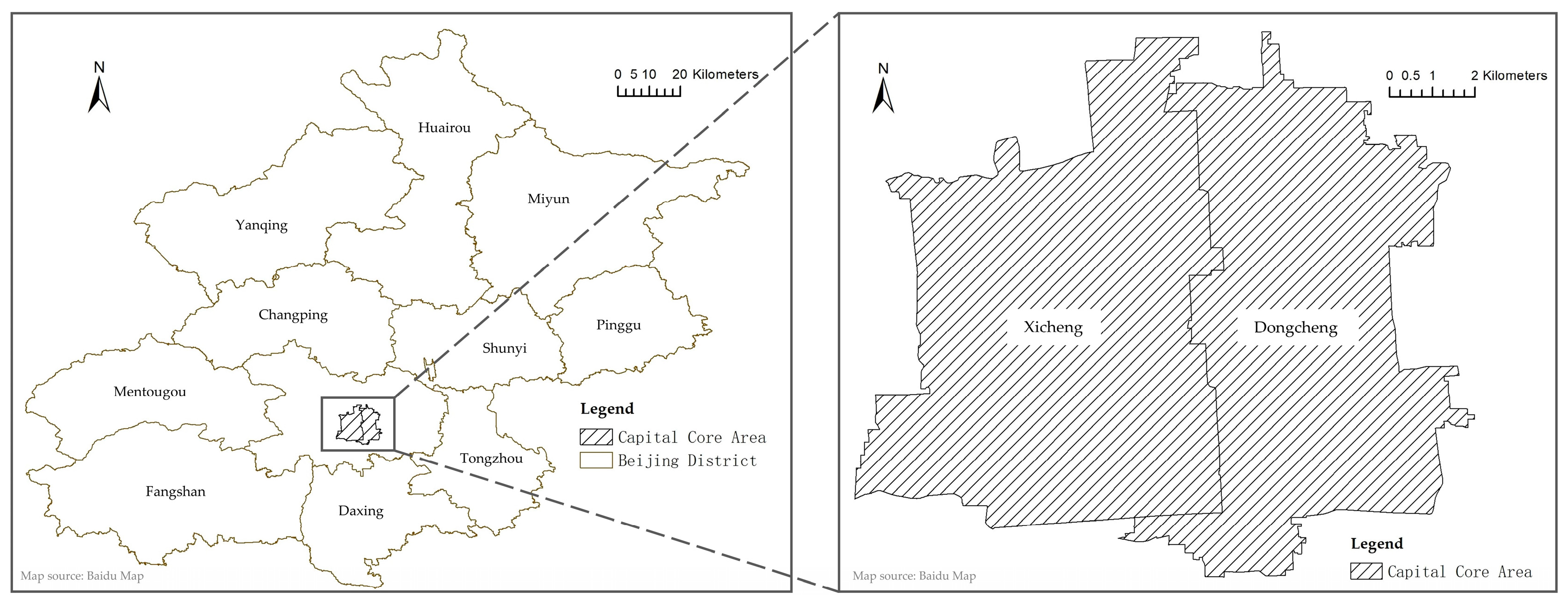
The Chinese information and communications technology (ICT) ecosystem provides advantageous conditions and a solid foundation for the development of shared mobility. The core area of Beijing, the capital of China, covers a total area of 92.5 square kilometers (Figure 1). It serves as the core bearing area for China’s political, cultural, and international communication center, and is also the most urbanized region in Beijing. The core zone of the capital, encompassing Dongcheng and Xicheng districts, hosts 60% of the permanent population and contributes to 70% of the GDP of Beijing [40]. In this context, the core area of Beijing not only experiences severe road congestion during peak periods but also deals with complex crowd flows throughout the rest of the day. Amidst the COVID-19 pandemic, the regular management of the epidemic has given rise to unique travel patterns and influencing factors for shared bicycles in the core area of Beijing. The State Council document “Detailed Control Planning (Neighborhood Level) of the Capital Function Core Area (2018–2035)” emphasizes the necessity to promote orderly traffic collection and decentralization of the core area of Beijing, along with the enhancement of traffic and travel guarantee mechanisms. Therefore, it becomes imperative to study the characteristics of shared bicycles and their influencing factors in the core area of Beijing, especially during the epidemic.
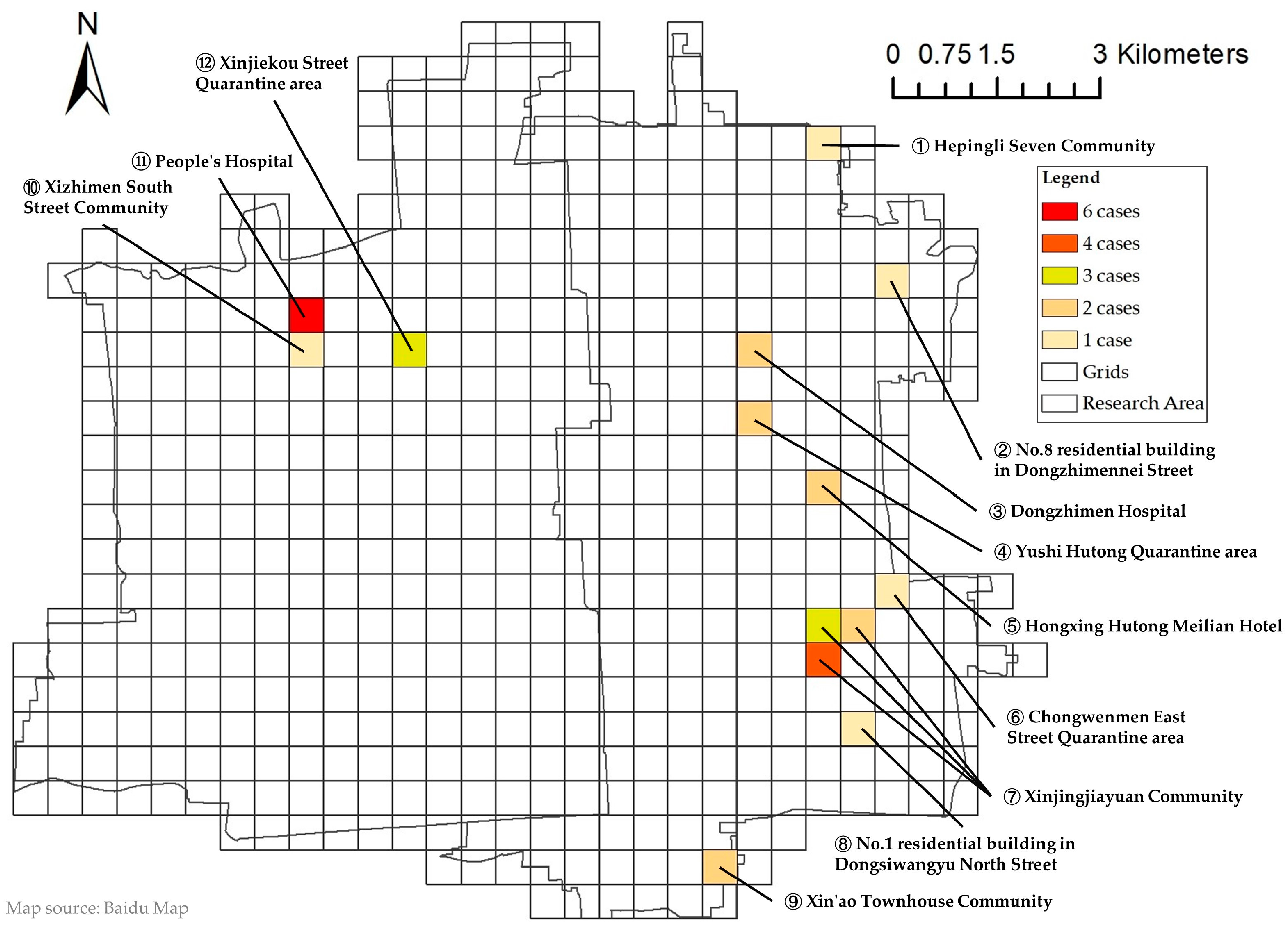
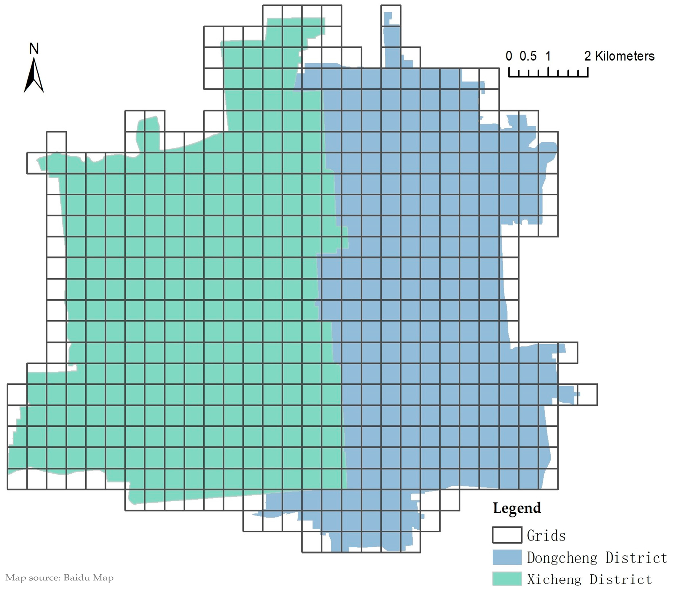
A vector-based polygonal grid is chosen as the spatial unit in this paper. The grid spatial framework has been tested and utilized in traffic alignment analysis, road safety analysis, and land use studies [41,42]. Unlike other spatial units with irregular shapes and variable sizes (such as streets, block groups, or traffic analysis zones), the regular grid can be employed in standard statistical spatial analysis [41], avoiding potential negative effects on results due to shape and size variations [43]. Considering that shared bicycles are typically used for short-distance travel, grids with large sizes may not adequately represent the characteristics of regional interaction, potentially canceling out travel within the grid. Conversely, grids with small sizes may result in the study area having fewer geographical attributes, which is not conducive to subsequent research. After extensive experimental validation, the decision was made to divide the study area into grids measuring 500 × 500 square meters. This grid system comprehensively covers the core area of Beijing (Figure 2). The grids within the region serve as network nodes, and the shared bicycle travel adjacency matrix is constructed using the polynomial network matrix, with values representing the shared bicycle outflow and inflow between grids.
The bicycle-sharing data utilized in this paper were sourced from a major bike-sharing company in Beijing. The data collection spanned from 17 to 21 October 2022, covering five consecutive typical working days. Each trip record includes detailed information such as trip ID, start and end times, start and end locations (latitude and longitude), trip duration, and an anonymized user ID. An example of the shared bicycle data is shown in Table 1. For example, a trip might start at 39.9123, 116.3976 (Beijing Union Hospital) and end at 39.9150, 116.4012 (Beijing Railway Station), with a duration of 10 min. The data were preprocessed to remove duplicates and aggregated into 500 m × 500 m grids for analysis. This preprocessing step ensured that the data were suitable for network-based analysis and allowed us to capture the spatial interactions between different areas of the city. Additionally, POI data were sourced from Baidu Maps and included categories such as hospitals, train stations, shopping centers, educational institutions, dining establishments, and financial services. An example of the POI data is shown in Table 2. For example, the POI data include locations such as Beijing Union Hospital (39.9123, 116.3976) and Peking University (39.9200, 116.4100). These POIs were integrated into the analysis to assess their impact on bike-sharing patterns, particularly during the COVID-19 pandemic.
Additionally, this paper utilized data from the Beijing zoning vector map, road network, and various types of points of interest (POI). The data of confirmed cases from 10 to 21 October 2022 were sourced from the Baidu epidemic real-time big data reporting website (https://voice.baidu.com/act/newpneumonia/newpneumonia (accessed on 22 October 2022)). The Beijing zoning data can be downloaded from the OpenStreetMap website (https://master.apis.dev.openstreetmap.org (accessed on 1 December 2022)). The POI data and road network data are available for download from Baidu Maps (https://map.baidu.com(accessed on 1 December 2022)). The details of the data used in this paper are presented in Table 3.

2.2. Research Methods

2.2.1. Travel Network Construction and Analysis with Spatial Grids as Nodes

Residents’ trips using shared bicycles in the city form an Origin–Destination (OD) flow constituting a complex network that illustrates spatial interactions between regions. In this paper, grids with a size of 500 m × 500 m serve as the network nodes, and the bicycle trips among the grids represent the edges, with the number of trips per period considered as the edge weights. To enhance accuracy, the shared bicycle location data underwent preprocessing involving the elimination of duplicate data and aggregation using the grid as the research unit. The working days were segmented into six time intervals for analysis: 0:00–4:00, 4:00–8:00, 8:00–12:00, 12:00–16:00, 16:00–20:00, and 20:00–24:00. The data for each of these time intervals were accumulated over the course of five days. The grid is instrumental in determining the origin and destination of bicycles’ OD flows. The origin and destination locations are linked with shared bike IDs to generate OD flows for multiple periods. Consequently, a travel network association matrix for these six time intervals was constructed.
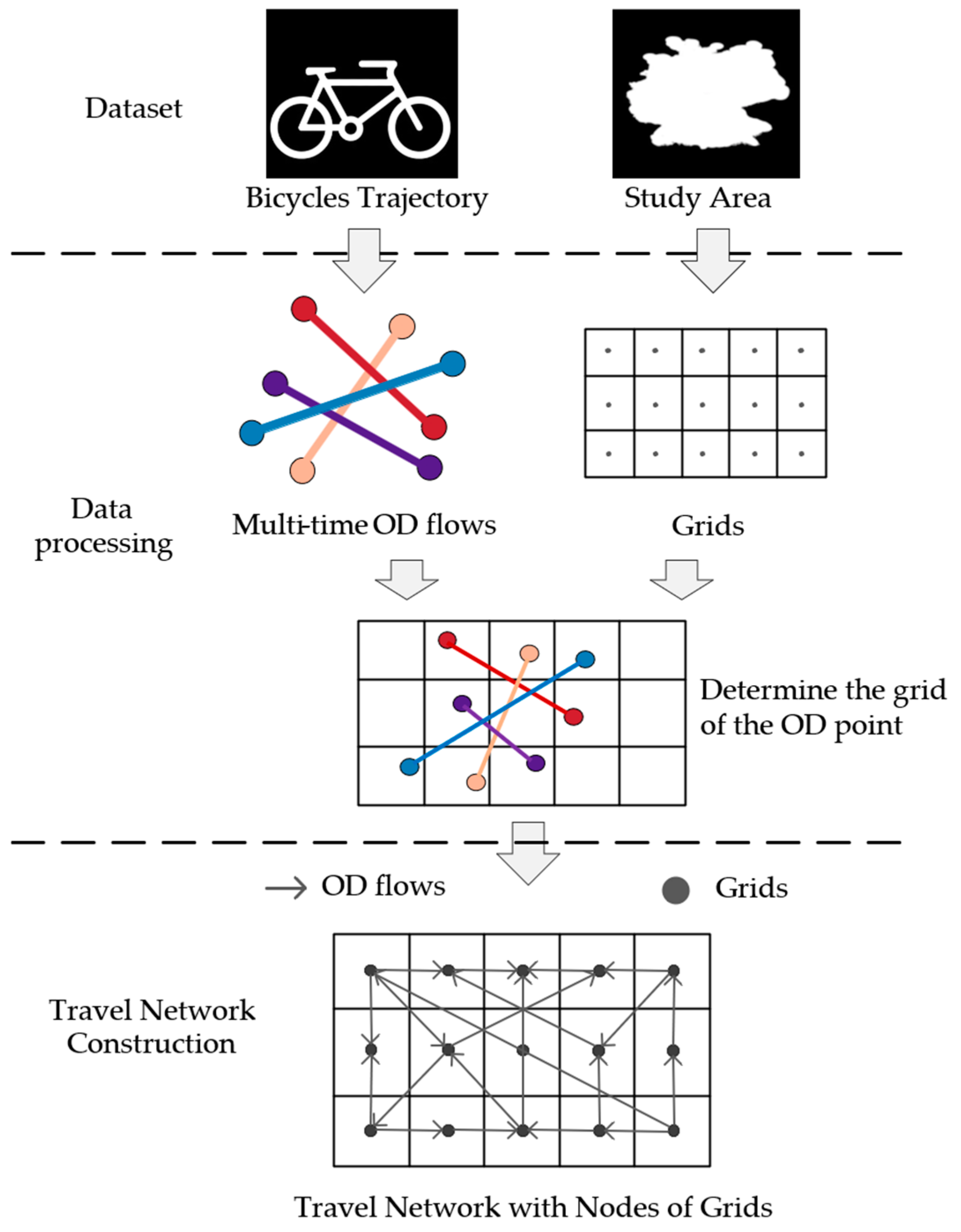
This matrix represents the travel network, where rows correspond to origin grids, columns to destination grids, and each element indicates the number of trips between an origin and destination during a specific time period. Each 500 m × 500 m grid serves as a node in the network, and travel activities form a directed network. Directed edges between nodes represent travel behaviors, with the edge direction indicating the travel direction and the edge weight corresponding to the trip volume. By mapping bike-sharing trip IDs to their start and end locations, we assign each trip to its corresponding origin and destination grids based on their geographic coordinates. Travel trajectories are then established between the grids. To improve visualization, grid centroids are used as node representations, and the network structure is finalized by connecting these nodes with directed edges that follow the street layout (Figure 3).
The travel network can be evaluated using network density and node strength. Network density indicates the level of interaction among nodes, with higher values signifying stronger connections and greater mutual influence. Here, D represents network density, k denotes the number of nodes, and d represents the total edges within the network. The calculation formula is provided in Equation (1).
D = d k k 1
Node strength refers to the total weight of all edges linked to a specific node, as defined in Equation (2). Here, node strength refers to the total weight of all edges linked to a specific node, as defined in Equation (2). Here, S i represents the strength of node i , N i is the set of nodes connected to i , and W i j is the weight of the edge between nodes i and j . In directed networks, node strength is further categorized into in-degree Sin(i) and out-degree Sout(i) based on edge direction. This distinction enables the calculation of the Net Flow Ratio (NFR) for nodes, with corresponding formulas provided in Equations (3)–(5).
S i = j N i W i j
S i n i = j ν i n W i j
S o u t i = j ν o u t W i j
N F R = S i n i S o u t i S i n i + S o u t i
S i n i and S o u t i represent the incoming and outgoing intensities of node i , respectively. ν i n is the set of nodes directing the flow to node i , while W i j is the weight of the edge between nodes i and j . ν o u t is the set of nodes that node i directs flow to, and N F R denotes the net flow ratio. When the N F R is positive, the incoming intensity exceeds the outgoing intensity, indicating an increase in the connection strength between nodes; if the N F R is negative, the connection strength decreases.

2.2.2. Travel Network Determinant Analysis with ERGM

The Exponential Random Graph Model (ERGM) offers a statistical approach to network modeling, focusing on the structural characteristics of a network. Unlike conventional descriptive methods, ERGM provides insights not only into the visible attributes of the network but also into the processes driving its formation. While other models, such as the gravity model and OD-focused spatial econometric models, are widely used for estimating OD flows, ERGM is particularly suited for capturing the complex interdependencies and network dynamics inherent in bike-sharing travel patterns. The gravity model, for example, is effective in predicting flow volumes based on distance and attractiveness factors, but it does not account for the network structure and interdependencies between regions. Similarly, OD-focused spatial econometric models are useful for analyzing spatial dependencies but may not fully capture the directional and weighted nature of bike-sharing networks. By employing ERGM, we are able to model both the network structure and the influence of node attributes, providing a more comprehensive understanding of the determinants of bike-sharing travel patterns during the COVID-19 pandemic [44,45]. This framework can accommodate both directed and weighted interactions between nodes, offering a deeper understanding of network dynamics [46]. In ERGM, the network is represented by a random graph G = V , E , where M i , j denotes the directed edge from node i to node j . The adjacency matrix M = [ M i , j ] captures the pairwise relationships between all nodes. Each matrix element M i , j represents the presence or absence of an edge between nodes i and j . The likelihood of a specific network configuration, denoted as m , occurring under a given set of parameters θ is represented by P θ M = m . This probability is influenced by the network statistics embedded in the model, which define the underlying structural characteristics of the network. The general and simplest form of ERGM is shown in Equation (6).
P θ M = m = 1 k exp H θ H g H m
Here, H is a collection of network statistics, and g m corresponds to the network statistic associated with the configuration m . The parameter θ reflects the weight of each statistic’s influence on the overall network structure. To estimate the model parameters, simulations of random graphs are generated, and the parameter values are refined by comparing the simulated networks with actual observed networks. This iterative process continues until the simulated network closely resembles the observed network structure. The constant k serves as a normalization factor to ensure that the probabilities across all possible network configurations sum to 1. The calculation equation is shown in Equation (7).
k = m exp H θ H g H m
In this formula, k ensures the consistency of the parameter estimates, normalizing the influence of the various network statistics on the network structure. By adjusting for these statistical variables, the model provides a robust framework for understanding the formation of travel networks.

2.2.3. Pandemic Impact Analysis of the Candidate Explanatory Variable in the Travel Network

This paper identifies two primary categories of network explanatory variables. The first category consists of pure network structure variables, which influence the development and organization of network relationships [47]. These variables represent various aspects of the network’s structure, such as edges, mutuality, closure, transitivity, k-triangles, and k-paths. In the ERGM framework, edges and mutuality are fundamental variables that capture different aspects of the network structure. Edges represent the basic connections between nodes, providing a measure of network density, while mutuality captures the likelihood of bidirectional interactions, which is crucial for understanding the reciprocity in directed networks. Based on empirical analysis and previous studies [48], this paper focuses on edges and mutuality as the selected explanatory variables.
The other category is node attribute variables. In the model of this paper, we include epidemic data, road network density, financial services, shopping places, dining places, transportation stops, transportation facilities, and educational institutions. For example, the POI data for dining places include locations such as Haidilao Hot Pot (39.9220, 116.4150), while educational institutions include Peking University (39.9200, 116.4100). These variables were integrated into the ERGM to assess their impact on bike-sharing patterns during the pandemic, as the epidemic has had a dramatic impact on people’s mobility. Strict control measures have reduced the number of people choose public transportation, and bike-sharing has thus become a major alternative for short-distance trips [49]. Bicycling during epidemics is also effective for users’ health expectations [36]. Due to the ongoing impact of the outbreak and relevant policies, the area where a case is located is identified as a high-risk area for one to two weeks. Therefore, the epidemic data collection period includes the shared bike data collection period (17–21 October 2022) and extends to seven days prior (10–16 October 2022). The location data of confirmed cases were collected from the Baidu epidemic big data report, which provides the geographic coordinates (latitude and longitude) of each case. These coordinates were used to assign cases to the corresponding 500 m × 500 m grids. For example, a case reported at 39.9123, 116.3976 (Beijing Union Hospital) was assigned to the grid containing these coordinates. The number of confirmed cases in each grid was then used as input to the model. While the number of cases is relatively small, it is representative of the spatial distribution of COVID-19 during the peak impact period in Beijing’s core area. We acknowledge that the limited number of cases may affect the generalizability of the findings, and future studies could benefit from a larger dataset covering a longer time frame. Although most grids in the study area had no COVID-19 cases during the data collection period, the presence of cases in certain grids can still significantly impact bike-sharing patterns. For example, areas with confirmed cases may experience reduced bike-sharing usage due to fear of infection, or they may experience increased usage as residents avoid public transportation. Therefore, the COVID-19 variable is included to capture the localized impact of the pandemic on bike-sharing behavior. Financial services have garnered significant interest from economic geographers due to their substantial productivity growth within the modern urban service sector [50]. However, previous research on shared bicycle travel patterns has seldom addressed the impact of financial services [14]. On the other hand, studies have shown a strong positive correlation between the presence of cafes and restaurants and the frequency of bike-sharing trips [23]. Areas with a high concentration of shopping malls and restaurants tend to experience greater demand for bike-sharing services [51]. Additionally, the accessibility of public transport stops plays a crucial role in enhancing the appeal of public transportation [52]. Financial services, as one of the influencing factors, have widely attracted the attention of economic geographers. As an important means of transportation to public transport stations, traffic stops are also essential to the volume of shared bicycle trips [22]. Distinguished from transportation stops, transportation facilities include infrastructure such as intersections, street lights, and traffic signals. Several studies have found that transportation facilities significantly impact bike-sharing trips [25,27]. Educational institutions are one the essential destinations for weekday trips and have a positive effect on shared bicycle travel activities [51]. The road network layout of the core area of Beijing originated in the Yuan Dynasty, with the Forbidden City as the center to set up a central axis running north and south. This central axis is used as the axis of symmetry to build a checkerboard-style road network. This road network layout can provide safe driving conditions for transport travel. However, this will lead to various detours from the departure point to the destination, and multiple road intersections will also affect the smooth flow of the traffic. In this paper, the total length of the road network in the grid is used as the input to the model.
Due to the data limitations of this study, factors such as weather, temperature, and precipitation are not considered in this paper. The definitions of the influencing factors and their measurement units in the model are shown in Table 4.

2.2.4. Integrated Method

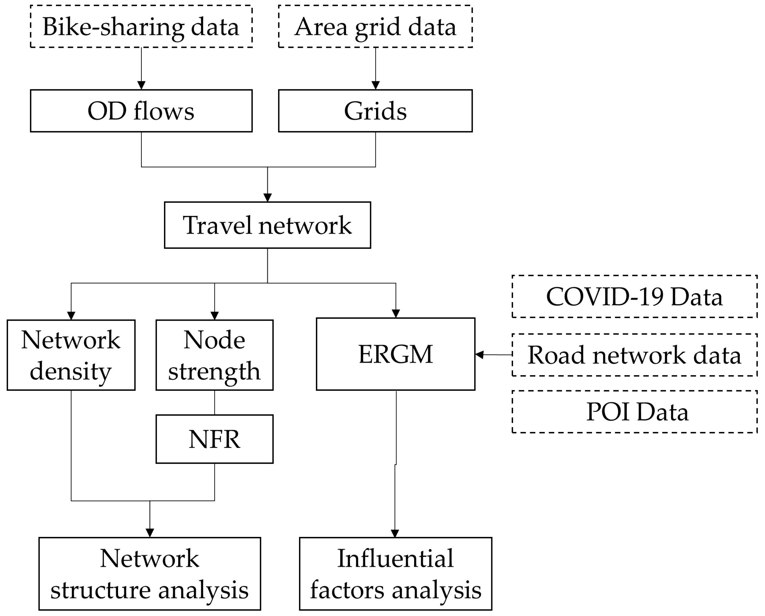
Firstly, the travel network was constructed based on the shared bikes and area grid data. Then, the travel network was analyzed from the perspective of network structure, network density, and node strength. Finally, COVID-19 data, road network data, and various types of POI data were input into ERGM as influencing factors to verify the effects of each factor. The experimental flow chart (Figure 4) illustrates the step-by-step process of this study as follows: (i) Data preparation: Shared bike data, POI data, road network data, and COVID-19 case data are collected and preprocessed; (ii) Network construction: The travel network is constructed using 500 m × 500 m grids as nodes, with shared bike trips forming the edges; (iii) Network analysis: Network density and node strength are calculated to analyze the spatial patterns of bike-sharing trips; (iv) ERGM modeling: The Exponential Random Graph Model (ERGM) is applied to identify the determinants of bike-sharing travel patterns, incorporating factors such as COVID-19 cases, road network density, and POIs.

3. Results

3.1. The Pandemic Situation in the Core Area of Beijing

To account for the unique characteristics of public health emergencies, particularly the ongoing impact of the COVID-19 pandemic, location data of confirmed cases were collected from 10 to 21 October 2022. The COVID variable represents the cumulative number of confirmed COVID-19 cases within each 500 m × 500 m grid during the data collection period (10 to 21 October 2022). This variable captures the overall impact of the pandemic on bike-sharing patterns in different areas, as the cumulative number of cases reflects the long-term exposure of each grid to the pandemic. Figure 5 shows the total number of cases per grid in the study area and the information on the location of the cases. The order and meaning of the numbers are consistent with Figure 5. Figure 5 show that the locations of confirmed cases were mostly residential communities (No. 1, 2, 7, 8, 9, 10), quarantine areas (No. 4, 6, 12), hotels (No. 5), and hospitals (No. 3, 11). The single grid with the highest total number of cases was the People’s Hospital. All three grids within the Xinjingjiayuan community had confirmed cases, and this community had the highest total number of cases during the experimental period.

3.2. Spatial Pattern Analysis of Multiple Periods During the Pandemic

3.2.1. Network Structure and Pandemic Effects Analysis During Multiple Periods

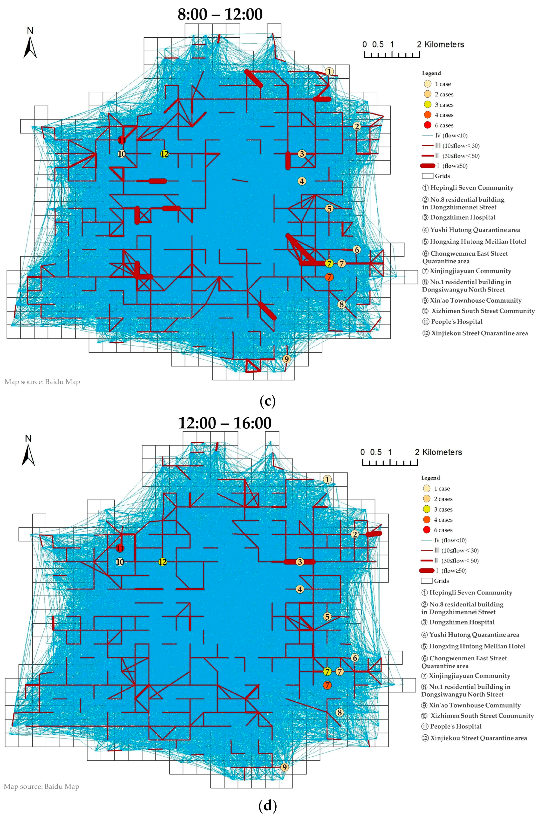
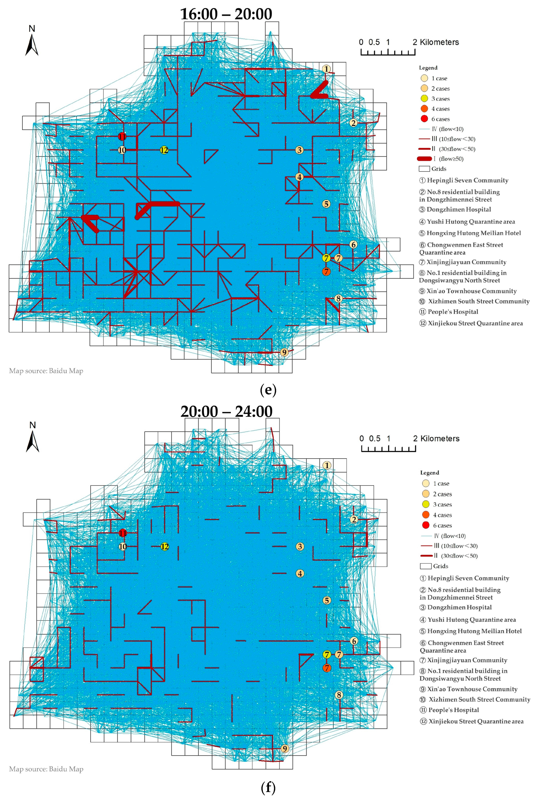
The bike-sharing travel networks were constructed for multiple periods, which were 0:00–4:00, 4:00–8:00, 8:00–12:00, 12:00–16:00, 16:00–20:00, and 20:00–24:00 (Figure 6a–f). Figure 6 illustrates the travel networks for the six different time periods. Figure 6a–f represents the bike-sharing flow patterns during a specific time slot. The blue lines in Figure 6a–f represent the directed edges between nodes (500 m × 500 m grids), with the thickness of the lines indicating the volume of bike-sharing trips. Thicker lines correspond to higher traffic volumes, while thinner lines represent lower traffic volumes. Key nodes, such as hospitals and train stations, are highlighted to show areas with significant travel activity. For example, in Figure 6b (4:00–8:00), the morning peak period, thicker lines are observed around residential areas and transportation hubs, indicating high commuting activity. In contrast, Figure 6f (20:00–24:00) shows thinner lines, reflecting lower traffic volumes during the nighttime period. The number of confirmed COVID-19 cases in each grid is indicated by the color of the nodes, with darker colors representing grids with more cases. The order and meaning of the node numbers are consistent with those shown in Figure 5. The network indicators were calculated in Table 5. To assess the statistical significance of the observed differences in network density and other indicators across time periods, we conducted paired t-tests. The results of these tests are presented in Table 6, which shows that the differences in network density between peak periods (e.g., 4:00–8:00 and 16:00–20:00) and off-peak periods (e.g., 0:00–4:00 and 20:00–24:00) are statistically significant (p < 0.05). This confirms that the observed differences are not merely statistical noise but reflect meaningful variations in bike-sharing usage patterns.
The bike-sharing travel networks were constructed for multiple periods, which are 0:00–4:00, 4:00–8:00, 8:00–12:00, 12:00–16:00, 16:00–20:00, and 20:00–24:00 (Figure 6a–f). The coordinates of the nodes are the geometric centers of the divided grids. The number of confirmed cases of COVID-19 is indicated using different-colored nodes. The order and meaning of the node numbers are consistent with those in Figure 5. The network indicators are calculated in Table 5.
Most network travel activities occurred between adjacent grids (Figure 6). Shared bicycles are usually used for short weekday trips, which is consistent with the travel characteristics of shared bicycles [14]. There are differences in bike-sharing usage during different periods. It can be seen that the nodes numbers in the travel network change during different periods. Figure 6 and Table 7 show that the four time periods (4:00–8:00, 8:00–12:00, 12:00–16:00, 16:00–20:00) are similar in terms of edge weights, number of nodes, network density, and total trips (total number of edges) in the network. Meanwhile, 0:00–4:00 and 20:00–24:00 differ significantly from these four time periods based on the indicators mentioned above. Therefore, for the spatial pattern analysis, we divided the six time periods into two time categories to conduct the analysis: the daytime period from 4:00–20:00 and the nighttime period from 0:00–4:00 and 20:00–24:00.
During the daytime, (i) 4:00–8:00 had the most significant number of nodes (Figure 6b) and more flow in level (I) than the remaining three periods during the daytime period (Figure 6). However, the network density and the total number of network edges in this period were the least. This shows the geographically concentrated characteristics in this time period. Since the 4:00–8:00 period is the morning peak for weekday travel, the purpose of travel during this period is mostly for commuting. Residents use shared bicycles more intensively to travel from their living places to workplaces or other public transportation transfer points. (ii) For 8:00–12:00 compared to 4:00–8:00, the network density and the total number of network edges were increased (Figure 6c). The traffic in level (I) decreased but remained high compared to the other time periods. This indicates that the traffic of residents is still concentrated during this time period, and the residents’ travel for commuting purposes still continues. (iii) The period of 12:00–16:00 is the most dispersed during the daytime. The amount of level (I) traffic is low, as well as the number of network edges and the network density (Figure 6d). This period is the transition time between morning and evening commutes. (iv) The period of 16:00–20:00 is the most active regarding bike-sharing use (Figure 6e). This is the evening peak period of the weekdays, when the network structure is significantly different from the morning peak, and the traffic distribution is relatively dispersed. The amount of traffic in level (I) is significantly less than the amount during the periods of 4:00–8:00 and 8:00–12:00. Meanwhile, it has the largest network density and total travel volume of the day. The results can be attributed to the reduction in commuting trips during this period, which also highlights the diverse leisure activities of residents in central Beijing during the COVID-19 pandemic. Additionally, bike-sharing usage remained steady throughout weekdays, with no notable peaks or dips. This consistent pattern is likely due to the high population density and urbanization in the study area, which encourages continuous movement of people within the city during the day.
At nighttime, the network structure during the periods of 0:00–4:00 and 20:00–24:00 does not have edges with larger weights, and the flows are very dispersed (Figure 6f). Furthermore, the number of nodes, network density, and total travel volume is significantly lower than during the daytime. For the bike-sharing operation, companies usually dispatch bikes at night to dispatch more bikes to the areas with high demand the next day. Therefore, the traffic during the nighttime period should be composed of sporadic trips by residents as well as bicycle dispatching.
Finally, we focus on the effects of the pandemic on the spatial patterns of the traffic network. The network structure shows that higher traffic volumes are sometimes present around the pandemic area at special times, i.e., during the periods of 4:00–8:00 and 12:00–16:00 for COVID-19 case No.3 and the period of 8:00–12:00 for case No. 7. Case No. 3 is located in Dongzhimen Hospital, and people in the surrounding area may choose to use shared bicycles to go to the hospital for epidemic prevention-related activities. Case No. 7 is located in the Xinjingjiayuan community; it is a large community with high travel demand, and it is near the Beijing Railway Station.

3.2.2. Network Degree, NFR, and Pandemic Effects Analysis During Multiple Periods

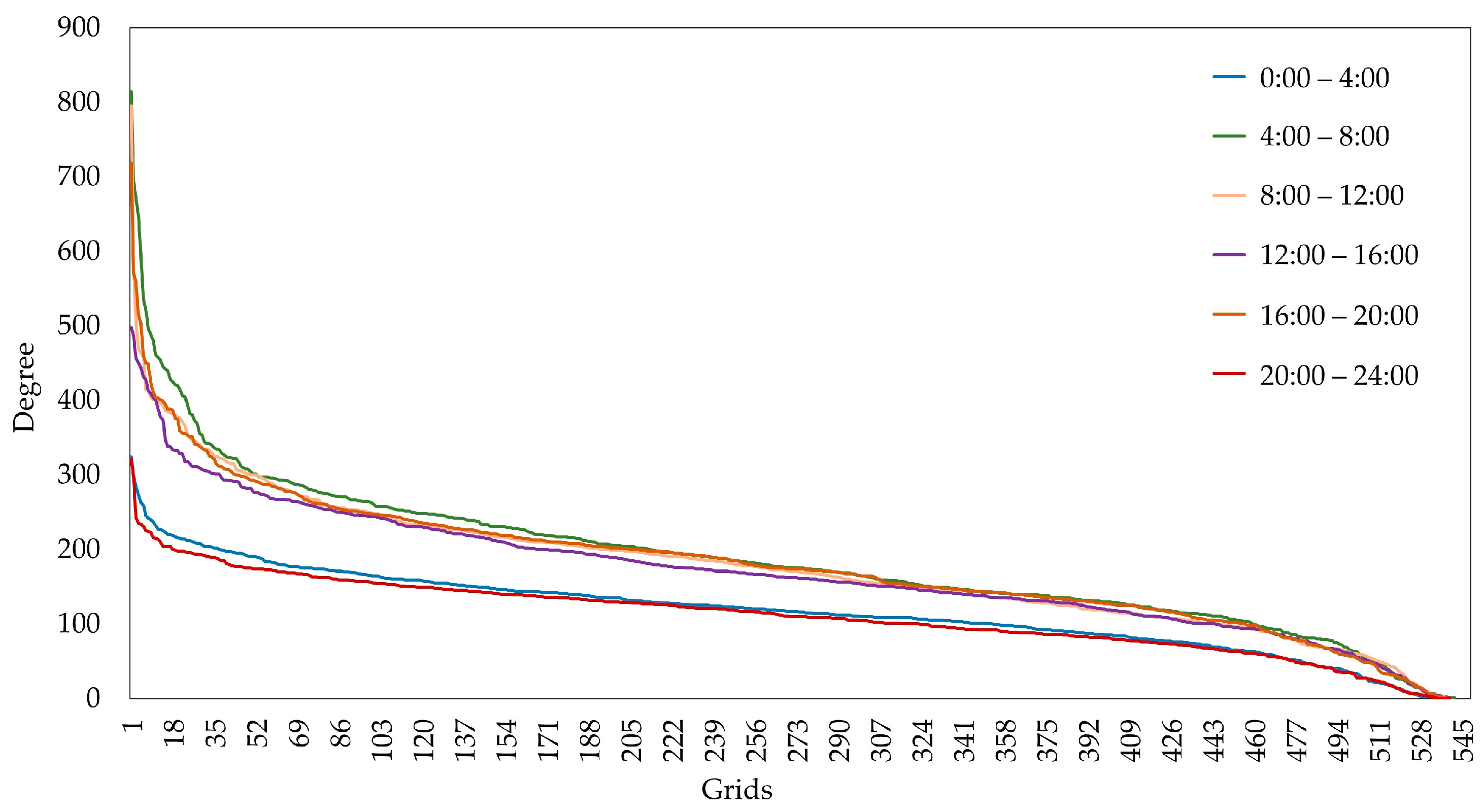
The degree and NFR of all nodes are calculated as shown in Figure 7 and Figure 8. The in-degree and out-degree of the nodes are summed to calculate the node intensities. The node intensity of all grids was calculated for each time period, and the grids were sorted from highest to lowest intensity. The X-axis in Figure 7 represents the sorted grid IDs, while the Y-axis shows the corresponding node intensity values. This ranking allows us to compare the relative importance of grids across different times of the day. The node intensity distribution of all time periods conforms to the power-law distribution and satisfies the scale-free property of the complex network. It can be clearly seen that the node intensities in the daytime period (4:00–20:00) are significantly higher than those in the nighttime period (0:00–4:00 and 20:00–24:00). The node intensity during 4:00–8:00, as the morning peak of urban travel, is slightly higher than the rest of the daytime periods. 12:00–16:00, as the transition time, is slightly lower than the rest of the daytime periods. The above findings verify the results of the network structure analysis in Section 3.2.1.
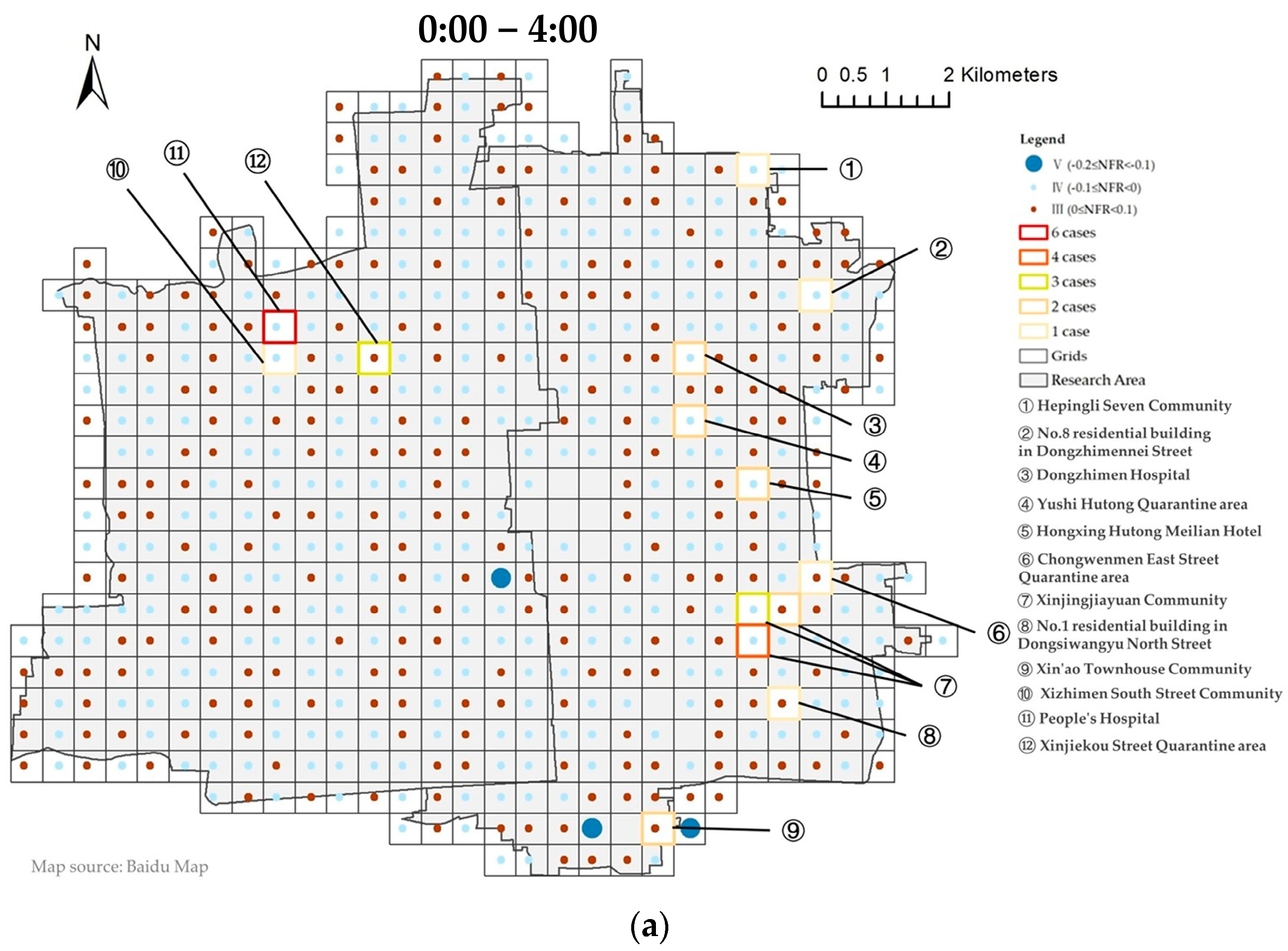
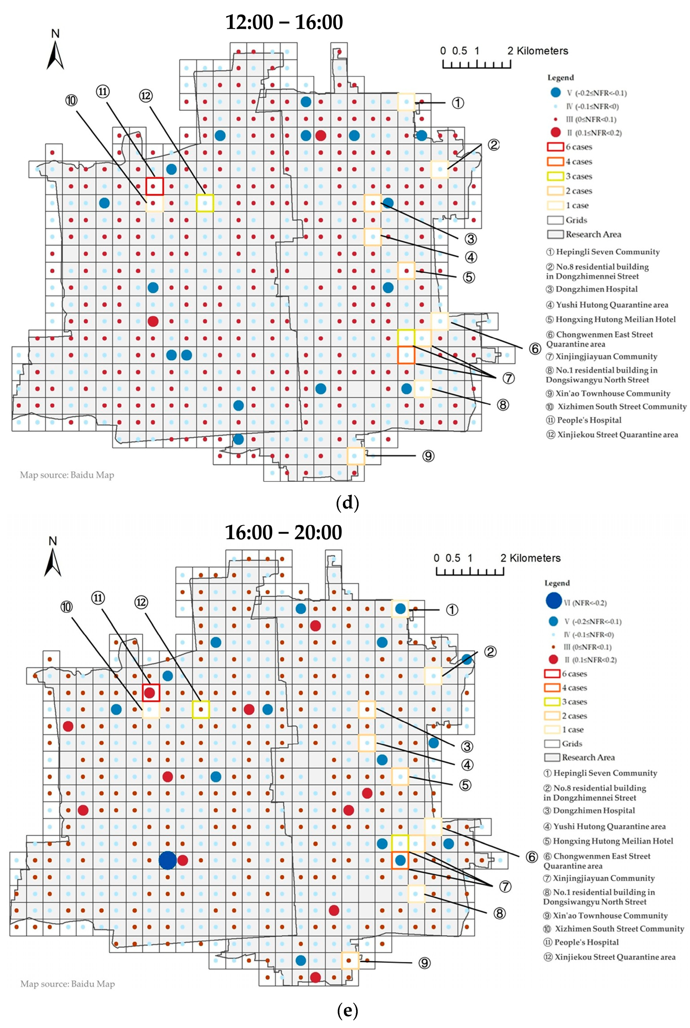
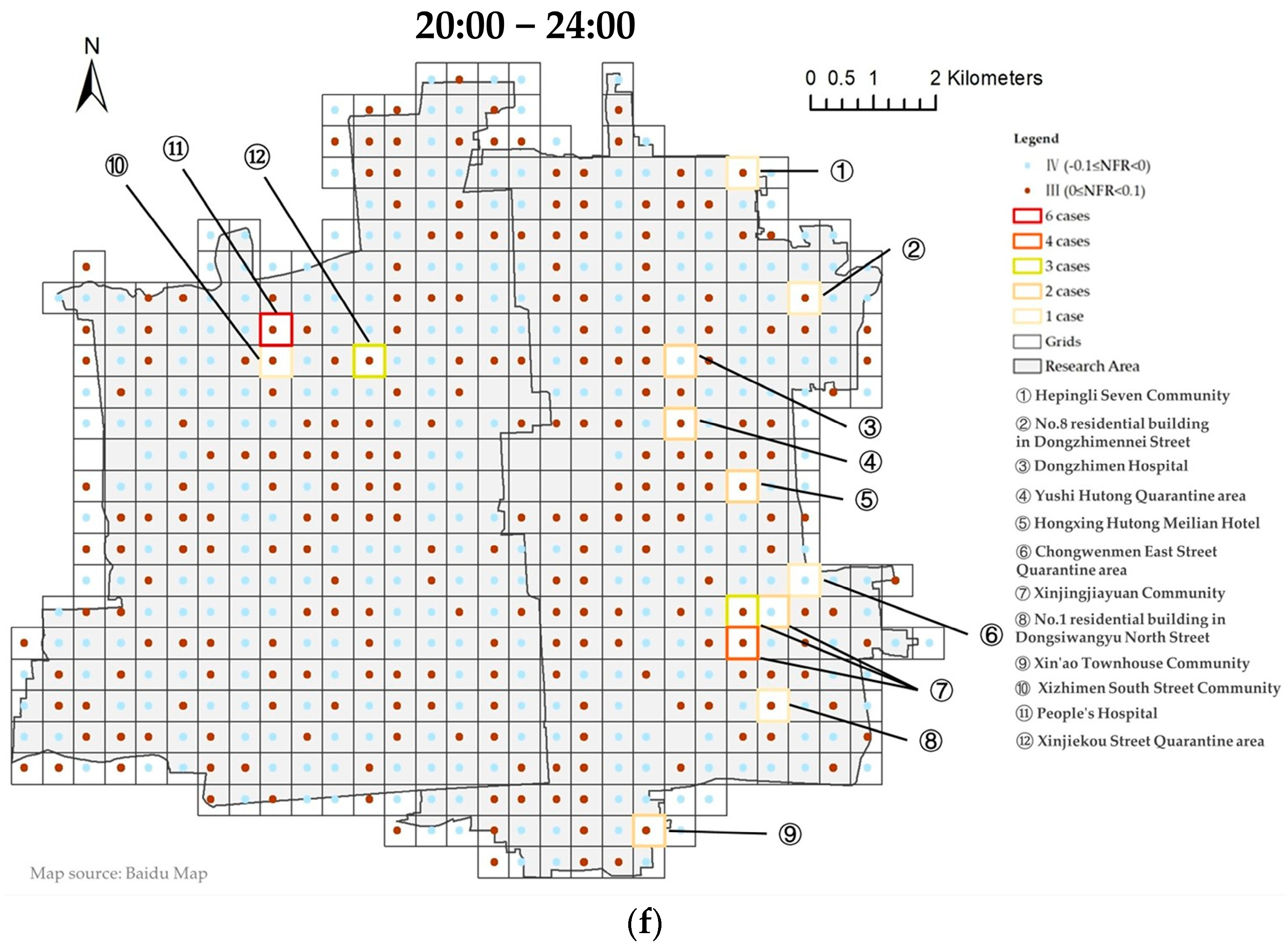
Figure 8 illustrates the spatial distribution of Net Flow Ratio (NFR) across the six time periods: 0:00–4:00, 4:00–8:00, 8:00–12:00, 12:00–16:00, 16:00–20:00, and 20:00–24:00. Figure 8a–f represents the NFR heat changes during a specific time slot. The grid was classified, and the variation in node heat was measured based on the attribution of NFR. The NFR values are classified into six intervals: (I), (II), (III), (IV), (V), and (VI). Levels (I), (II), and (III) represent NFR values greater than zero, indicating an increase in heat, and they are shown in red, with (III) being the level with the highest NFR value. Levels (IV), (V), and (VI) represent NFR values less than zero, indicating a decrease in heat, and they are shown in blue, with (VI) being the level with the most significant negative NFR value. Additionally, the number of confirmed COVID-19 cases is represented by grids of different colors, with the order and meaning of the node numbers consistent with Figure 5. From Figure 8, we can analyze the following results: Key areas with notable NFR values, such as grids with the highest increases or decreases in heat, are annotated to help readers quickly locate and interpret important patterns. For example, in Figure 8b (4:00–8:00), the morning peak period, areas around residential neighborhoods and transportation hubs show significant decreases in heat, reflecting residents leaving for work or transit points. In contrast, Figure 8e (16:00–20:00), the evening peak period, shows more dispersed heat changes, with some areas experiencing increases in heat due to diverse travel purposes such as leisure and dining.
Firstly, we focus on the network NFR during the daytime periods. (i) The period of 4:00–8:00 is the primary period of the morning peak with the highest concentration of heat changes (Figure 8b). It includes one node of level (I), four nodes of level (VI), and several nodes of levels (II) and (V). There are more nodes with a decrease in the heat than an increase during this period. People leave their residences in the morning peak to work or change to other public transportation methods. Therefore, most of the nodes with a decrease in NFR heat should be areas with a high concentration of residences and high crowd density during this period. (ii) The period of 8:00–12:00 includes nodes of level (II) to level (VI) (Figure 8c). These include one level (VI) node and many level (II) and (V) nodes. As shown in the analysis of network structure, the residents’ travel continues during this period, but it is clear that the peak period of commuting has passed. The number of nodes with increases and decreases in travel heat during this period is almost equal, and the use of shared bicycles is active. (iii) The period of 12:00–16:00 includes the nodes from level (II) to level (V) (Figure 8d). Since this period is a transition time for morning and evening commuting, few nodes with significant heat variations exist. There are significantly more nodes in level (V) than in level (II) during this period. The heat of nodes in this period is mainly decreasing. (iv) The period of 16:00–20:00 includes nodes of level (I) to level (VI). This is the main period of the city’s mid-evening peak (Figure 8e). It includes one node of level (I) with multiple nodes of levels (II) and (V). Unlike the morning peak of 4:00–8:00, there are more nodes with increased heat, and node heat is relatively dispersed during this period. Thus, this indicates that residents do not return to their residences in a concentrated manner during the evening peak period. They are more likely to travel to other destinations, i.e., the purposes of their trips are more varied, which is consistent with the results of the network structure analysis.
Secondly, we focus on the nighttime periods. The periods of 0:00–4:00 and 20:00–24:00 are the two periods when most nodes have NFR values close to 0, including only levels (III), (IV), and (V) (Figure 8a,f). Therefore, there are fewer trips and less variation in node heat during the nighttime period.
Finally, we focus on the effects of the pandemic. There were no obvious changes in NFR heat in the grids where outbreak cases were present during the periods of 0:00–4:00, 12:00–16:00, and 20:00–24:00. When the outbreak cases were present, the NFR values were all at levels (III) or (VI). Only case No. 10 during 4:00–8:00 and case No. 11 and No. 7 during 8:00–12:00 and 16:00–20:00 had NFR of levels (II) and (V). These three periods were also the most active periods of the day for bike-sharing use. From the grid location information in Table 3, we can see that case No. 10 was in the Xizhimen South Street neighborhood and case No.11 was near the People’s Hospital. These two locations are close, and there is a high probability that the trip purpose of these two grids was related to the hospital.

3.3. Pandemic Impact Analysis on the Network Determinants

The ERGM models were constructed using R (4.1.3) software, with the model and source code available for download at https://github.com/statnet/ergm (accessed on 21 November 2021). The ERGM results are presented in Table 7, which provides insights into the formation of the travel network. The table shows the coefficient values, with the corresponding standard errors in parentheses, and the parameter P for hypothesis testing [53]. To assess the model’s fit, the Akaike Information Criterion (AIC) and the Bayesian Information Criterion (BIC) were used, with smaller values of AIC and BIC indicating a better model fit. Based on the data in Table 7, the following conclusions can be drawn.
Secondly, our analysis focuses on the nodal attribute variables. (1) It is noteworthy that Rnet (Road network) is always the factor with the most significant influence on bike-sharing trips. Regardless of the different periods, it always showed a significant negative coefficient (Table 7). And, the influence was significantly greater in the daytime than in the nighttime. This shows that the complexity of the road is the most important factor in whether travelers use shared bikes. If the roads are too complicated, travelers may choose other travel methods, since the values of the road network coefficients are significantly higher—by orders of magnitude—than the other factors. In order to avoid its visual impact on the other factors in the bar chart, we only show the coefficient values of the remaining six factors in Figure 9a. (2) As shown in Figure 9a, Covid (COVID-19 epidemic cases) shows a significant positive coefficient in the daytime period. It shows a significant influence during the COVID-19 epidemic. This influence becomes progressively greater from 4:00 to 16:00 and reaches a maximum at 12:00–16:00, then it starts to decrease. Therefore, in areas with more COVID-19 epidemic cases, people would be more likely to use bike-sharing to travel to reduce the likelihood of infection, which is consistent with previous studies [36,37]. Similarly to the above, only the coefficient values of five factors other than road network and epidemic are shown in Figure 9b. (3) Tsta (Transportation stops) and Edu (Education institutions) have positive coefficients during daytime (Figure 9b). This indicates that transportation stops and educational institutions have a facilitating effect on shared bicycle trips. Regarding the degree of influence, the coefficient of Edu is higher, indicating that the influence of educational institutions is more significant. (4) Tfac (transportation facilities) has a negative coefficient at 20:00–24:00, and Fin (financial services) has a negative coefficient at 0:00–4:00, but both have positive coefficients during the daytime (Figure 9b). It can be shown that transportation facilities and financial services facilitate bike-sharing trips during the daytime. The degree of influence of transportation facilities is significantly smaller than that of transportation stops, educational institutions, and financial services. (5) The coefficients of Din (dining facilities) and Shop are both small (Figure 9b). Din has a positive coefficient only during the periods of 0:00–4:00 and 8:00–12:00, indicating that dining facilities generally have a negative effect on shared bicycle trips during weekdays. In comparison, there may be more trips for dining purposes from 8:00 to 12:00 p.m. The coefficient of Shop is significantly higher during the nighttime than during the daytime period. This indicates that shopping places are less attractive for bike-sharing trips during the daytime period.

4. Discussion

Based on bike-sharing data, this study investigated the spatial and temporal variations of travel networks in Beijing’s core area during the COVID-19 pandemic, with a particular focus on weekdays. By utilizing network structure indicators, we analyzed the travel characteristics of bike-sharing and applied the Exponential Random Graph Model (ERGM) to explore the factors influencing the formation of urban bike-sharing travel networks during the pandemic. Our findings emphasize the significant impact of COVID-19 on bike-sharing usage patterns, especially in areas with high infection rates. The main findings and their implications for urban mobility planning are as follows.
(i) The analysis reveals that bike-sharing is predominantly used for short-distance travel, with most trips occurring between adjacent grids. The travel patterns exhibit distinct temporal variations, divided into daytime (4:00–20:00) and nighttime (0:00–4:00 and 20:00–24:00) periods. Daytime travel is characterized by higher total trip volumes, broader usage ranges, and greater traffic concentration compared to nighttime. Specifically, 4:00–8:00 represents the morning peak, with the most concentrated traffic, followed by 8:00–12:00, where commuting continues. The period from 12:00 to 16:00 serves as a transition phase, while 16:00–20:00 marks the evening peak, the most active period for bike-sharing, with residents engaging in diverse travel purposes such as leisure and dining. Notably, bike-sharing maintains a consistent level of activity throughout the daytime, without significant peaks or valleys, reflecting the high population density and continuous urban mobility in Beijing’s core area. (ii) The node intensity distribution follows a power-law distribution, indicating that the travel network exhibits scale-free properties, a hallmark of complex networks. Node intensity is significantly higher during the daytime than at night. Within the daytime, 4:00–8:00 records the highest node intensity, while 12:00–16:00 has the lowest. The NFR analysis further reveals that 4:00–8:00 is the most concentrated period, with a dominant decrease in node heat, reflecting residents leaving residential areas for work or transit hubs. In contrast, 8:00–12:00 shows a balanced increase and decrease in heat, indicating sustained commuting activity. The evening peak (16:00–20:00) is more dispersed, with residents traveling for varied purposes, such as leisure and dining, rather than returning directly home. Nighttime periods exhibit minimal heat variation and lower trip volumes, likely due to reduced activity and bike rebalancing operations. (iii) The network structure, node strength, and NFR analysis indicate that bike-sharing usage in areas with confirmed COVID-19 cases is generally lower than in unaffected areas, likely due to reduced mobility and fear of infection. However, the presence of hospitals and train stations increases travel activity in pandemic-affected areas, as these locations remain essential for commuting and medical purposes. This highlights the dual role of bike-sharing during the pandemic: as a safer alternative to public transport and a critical mode of travel for essential activities. (iv) The ERGM results reveal that mutual connections (Mutual) have a significant positive effect, indicating a high likelihood of bidirectional interactions between node pairs. The road network (Rnet) is the most influential factor, with a strong negative impact on bike-sharing trips, suggesting that complex road layouts may deter bike usage. Conversely, the COVID-19 pandemic (Covid) has the most substantial positive influence during the daytime, as residents opt for bike-sharing to avoid public transport and reduce infection risks. Transportation stops (Tsta) and educational institutions (Edu) also play significant roles, with positive coefficients throughout the day, reflecting their importance as key destinations. Transportation facilities and financial services further boost bike-sharing during the daytime, while dining (Din) and shopping (Shop) have smaller effects. Dining establishments only facilitate trips during 8:00–12:00, likely due to lunch-related travel, but negatively impact bike-sharing at other times. Shopping establishments have a minor effect during the day but slightly higher activity at night, possibly due to leisure shopping.
These findings provide valuable insights into the dynamics of bike-sharing during public health emergencies, offering practical implications for urban transportation planning and bike-sharing system management. This study underscores the importance of optimizing bike allocation, enhancing infrastructure near key destinations, and addressing the unique challenges posed by pandemics to ensure sustainable urban mobility.

5. Conclusions

This study offers valuable insights into the dynamics of urban bike-sharing travel networks during the COVID-19 pandemic in Beijing. The key findings highlight the short-distance travel nature of bike-sharing, the significant impact of the COVID-19 pandemic on travel patterns, and the crucial role of transportation infrastructure, such as hospitals, train stations, and educational institutions, in shaping travel behavior. The Exponential Random Graph Model (ERGM) has proven essential in identifying the various factors influencing the formation and evolution of travel networks during the pandemic.
These findings have important practical implications for urban traffic management and bike-sharing operators, emphasizing the need for strategic adjustments in bike distribution, infrastructure, and scheduling to better align with shifting travel demand patterns during the pandemic. Specifically, bikes should be deployed more intensively in areas with high travel demand during peak periods and in locations with COVID-19 cases to mitigate infection risks. Future research should consider comparative analyses with alternative modeling approaches, expand the range of influencing factors included in the analysis, and refine the methods for accurately identifying network nodes to improve the robustness of findings.
Despite its valuable insights, this study has certain limitations, such as the reliance on a single model (ERGM), the short data collection period, and the potential simplification of network nodes. Future research could address these limitations by incorporating additional models, expanding the time window, and refining the node identification methods. Such improvements will enhance the robustness of the findings and provide more effective recommendations for pandemic prevention and urban mobility management.
Author Contributions

Zheng Wen performed the computations, verified the analytical methods, and carried out the experiments. Lujin Hu conceived of the presented idea and developed the theory. Jing Hu completed the data collection and data preprocessing. All authors discussed the results and contributed to the final manuscript. All authors have read and agreed to the published version of the manuscript.

Funding

This work was supported by the National Key Research and Development Program of China (Grant no. 2020YFD1100201) and Beijing University of Civil Engineering and Architecture’s young teachers research ability enhancement program (X21023).

Data Availability Statement

Data are contained within the article.

Conflicts of Interest

The authors declare no conflicts of interest.

References

  1. Shang, W.-L.; Chen, J.; Bi, H.; Sui, Y.; Chen, Y.; Yu, H. Impacts of COVID-19 Pandemic on User Behaviors and Environmental Benefits of Bike Sharing: A Big-Data Analysis. Appl. Energy 2021, 285, 116429. [Google Scholar] [CrossRef]
  2. Venter, Z.S.; Aunan, K.; Chowdhury, S.; Lelieveld, J. COVID-19 Lockdowns Cause Global Air Pollution Declines. Proc. Natl. Acad. Sci. USA 2020, 117, 18984–18990. [Google Scholar] [CrossRef]
  3. Jobe, J.; Griffin, G.P. Bike Share Responses to COVID-19. Transp. Res. Interdiscip. Perspect. 2021, 10, 100353. [Google Scholar] [CrossRef] [PubMed]
  4. Oum, T.H.; Wang, K. Socially Optimal Lockdown and Travel Restrictions for Fighting Communicable Virus Including COVID-19. Transp. Policy 2020, 96, 94–100. [Google Scholar] [CrossRef]
  5. Štefancová, V.; Kalašová, A.; Čulík, K.; Mazanec, J.; Vojtek, M.; Mašek, J. Research on the Impact of COVID-19 on Micromobility Using Statistical Methods. Appl. Sci. 2022, 12, 8128. [Google Scholar] [CrossRef]
  6. Kwak, J.; Oh, H.; Jeong, I.; Shin, S.; Ku, D.; Lee, S. Changes in Shared Bicycle Usage by COVID-19. Chem. Eng. Trans. 2021, 89, 169–174. [Google Scholar] [CrossRef]
  7. Padmanabhan, V.; Penmetsa, P.; Li, X.; Dhondia, F.; Dhondia, S.; Parrish, A. COVID-19 Effects on Shared-Biking in New York, Boston, and Chicago. Transp. Res. Interdiscip. Perspect. 2021, 9, 100282. [Google Scholar] [CrossRef] [PubMed]
  8. Shen, S.; Wei, Z.-Q.; Sun, L.-J.; Su, Y.-Q.; Wang, R.-C.; Jiang, H.-M. The Shared Bicycle and Its Network—Internet of Shared Bicycle (IoSB): A Review and Survey. Sensors 2018, 18, 2581. [Google Scholar] [CrossRef] [PubMed]
  9. Zhao, D.; Ong, G.P. Geo-Fenced Parking Spaces Identification for Free-Floating Bicycle Sharing System. Transp. Res. Part A Policy Pract. 2021, 148, 49–63. [Google Scholar] [CrossRef]
  10. Fishman, E. Bikeshare: A Review of Recent Literature. Transp. Rev. 2016, 36, 92–113. [Google Scholar] [CrossRef]
  11. Wang, J.; Huang, J.; Dunford, M. Rethinking the Utility of Public Bicycles: The Development and Challenges of Station-Less Bike Sharing in China. Sustainability 2019, 11, 1539. [Google Scholar] [CrossRef]
  12. Gao, K.; Yang, Y.; Li, A.; Li, J.; Yu, B. Quantifying Economic Benefits from Free-Floating Bike-Sharing Systems: A Trip-Level Inference Approach and City-Scale Analysis. Transp. Res. Part A Policy Pract. 2021, 144, 89–103. [Google Scholar] [CrossRef]
  13. Chen, Z.; van Lierop, D.; Ettema, D. Dockless Bike-Sharing Systems: What Are the Implications? Transp. Rev. 2020, 40, 333–353. [Google Scholar] [CrossRef]
  14. Hu, L.; Wen, Z.; Wang, J.; Hu, J. Spatial Interaction Analysis of Shared Bicycles Mobility Regularity and Determinants: A Case Study of Six Main Districts, Beijing. ISPRS Int. J. Geo-Inf. 2022, 11, 477. [Google Scholar] [CrossRef]
  15. Li, Y.; Zhu, Z.; Guo, X. Operating Characteristics of Dockless Bike-Sharing Systems near Metro Stations: Case Study in Nanjing City, China. Sustainability 2019, 11, 2256. [Google Scholar] [CrossRef]
  16. Crawford, F.; Watling, D.P.; Connors, R.D. A Statistical Method for Estimating Predictable Differences between Daily Traffic Flow Profiles. Transp. Res. Part B Methodol. 2017, 95, 196–213. [Google Scholar] [CrossRef]
  17. O’Brien, O.; Cheshire, J.; Batty, M. Mining Bicycle Sharing Data for Generating Insights into Sustainable Transport Systems. J. Transp. Geogr. 2014, 34, 262–273. [Google Scholar] [CrossRef]
  18. Garcia-Gutierrez, J.; Romero-Torres, J.; Gaytan-Iniestra, J. Dimensioning of a Bike Sharing System (BSS): A Study Case in Nezahualcoyotl, Mexico. Procedia-Soc. Behav. Sci. 2014, 162, 253–262. [Google Scholar] [CrossRef]
  19. Chen, X.; Ma, Z.; Ye, G.; Li, Z. Usage Behavior and Satisfaction Analysis of Free-Floating Bicycle Sharing System Service: Evidence from a Chinese University Campus. Res. Transp. Bus. Manag. 2022, 43, 100703. [Google Scholar] [CrossRef]
  20. Eren, E.; Uz, V.E. A Review on Bike-Sharing: The Factors Affecting Bike-Sharing Demand. Sustain. Cities Soc. 2020, 54, 101882. [Google Scholar] [CrossRef]
  21. Zhao, D.; Ong, G.P.; Wang, W.; Zhou, W. Estimating Public Bicycle Trip Characteristics with Consideration of Built Environment Data. Sustainability 2021, 13, 500. [Google Scholar] [CrossRef]
  22. Bachand-Marleau, J.; Lee, B.H.Y.; El-Geneidy, A.M. Better Understanding of Factors Influencing Likelihood of Using Shared Bicycle Systems and Frequency of Use. Transp. Res. Rec. 2012, 2314, 66–71. [Google Scholar] [CrossRef]
  23. Maas, S.; Nikolaou, P.; Attard, M.; Dimitriou, L. Heat, Hills and the High Season: A Model-Based Comparative Analysis of Spatio-Temporal Factors Affecting Shared Bicycle Use in Three Southern European Islands. Sustainability 2021, 13, 3274. [Google Scholar] [CrossRef]
  24. Maas, S.; Nikolaou, P.; Attard, M.; Dimitriou, L. Spatial and Temporal Analysis of Shared Bicycle Use in Limassol, Cyprus. J. Transp. Geogr. 2021, 93, 103049. [Google Scholar] [CrossRef]
  25. Faghih-Imani, A.; Eluru, N. Incorporating the Impact of Spatio-Temporal Interactions on Bicycle Sharing System Demand: A Case Study of New York CitiBike System. J. Transp. Geogr. 2016, 54, 218–227. [Google Scholar] [CrossRef]
  26. Duan, Y.; Zhang, S.; Yu, Z. Applying Bayesian Spatio-Temporal Models to Demand Analysis of Shared Bicycle. Phys. A Stat. Mech. Its Appl. 2021, 583, 126296. [Google Scholar] [CrossRef]
  27. Zacharias, J.; Meng, S. Environmental Correlates of Dock-Less Shared Bicycle Trip Origins and Destinations. J. Transp. Geogr. 2021, 92, 103013. [Google Scholar] [CrossRef]
  28. Wang, Z.; Cheng, L.; Li, Y.; Li, Z. Spatiotemporal Characteristics of Bike-Sharing Usage around Rail Transit Stations: Evidence from Beijing, China. Sustainability 2020, 12, 1299. [Google Scholar] [CrossRef]
  29. Kutela, B.; Teng, H. The Influence of Campus Characteristics, Temporal Factors, and Weather Events on Campuses-Related Daily Bike-Share Trips. J. Transp. Geogr. 2019, 78, 160–169. [Google Scholar] [CrossRef]
  30. Meng, S.; Zacharias, J. Street Morphology and Travel by Dockless Shared Bicycles in Beijing, China. Int. J. Sustain. Transp. 2021, 15, 788–798. [Google Scholar] [CrossRef]
  31. Teixeira, J.F.; Lopes, M. The Link between Bike Sharing and Subway Use during the COVID-19 Pandemic: The Case-Study of New York’s Citi Bike. Transp. Res. Interdiscip. Perspect. 2020, 6, 100166. [Google Scholar] [CrossRef] [PubMed]
  32. Chibwe, J.; Heydari, S.; Faghih Imani, A.; Scurtu, A. An Exploratory Analysis of the Trend in the Demand for the London Bike-Sharing System: From London Olympics to COVID-19 Pandemic. Sustain. Cities Soc. 2021, 69, 102871. [Google Scholar] [CrossRef]
  33. Hu, S.; Xiong, C.; Liu, Z.; Zhang, L. Examining Spatiotemporal Changing Patterns of Bike-Sharing Usage during COVID-19 Pandemic. J. Transp. Geogr. 2021, 91, 102997. [Google Scholar] [CrossRef] [PubMed]
  34. Elhenawy, M.; Komol, M.R.; Masoud, M.; Liu, S.Q.; Ashqar, H.I.; Almannaa, M.H.; Rakha, H.A.; Rakotonirainy, A. A Novel Crowdsourcing Model for Micro-Mobility Ride-Sharing Systems. Sensors 2021, 21, 4636. [Google Scholar] [CrossRef] [PubMed]
  35. Hu, J.-W.; Creutzig, F. A Systematic Review on Shared Mobility in China. Int. J. Sustain. Transp. 2022, 16, 374–389. [Google Scholar] [CrossRef]
  36. Saatchian, V.; Azimkhani, A.; Türkmen, M.; Laein, D.D. Cycling as Transportation & COVID-19: Advantages of Shared Bicycles during Epidemics. Sport Mont 2021, 19, 51–57. [Google Scholar] [CrossRef]
  37. Kubaľák, S.; Kalašová, A.; Hájnik, A. The Bike-Sharing System in Slovakia and the Impact of COVID-19 on This Shared Mobility Service in a Selected City. Sustainability 2021, 13, 6544. [Google Scholar] [CrossRef]
  38. Meng, F.; Zheng, L.; Ding, T.; Wang, Z.; Zhang, Y.; Li, W. Understanding dockless bike-sharing spatiotemporal travel patterns: Evidence from ten cities in China. Comput. Environ. Urban Syst. 2023, 04, 102006. [Google Scholar] [CrossRef]
  39. Zhang, H.; Zhuge, C.; Jia, J.; Shi, B.; Wang, W. Green travel mobility of dockless bike-sharing based on trip data in big cities: A spatial network analysis. J. Clean. Prod. 2021, 313, 127930. [Google Scholar] [CrossRef]
  40. Qiao, Z.; Xu, X.; Wu, F.; Luo, W.; Wang, F.; Liu, L.; Sun, Z. Urban Ventilation Network Model: A Case Study of the Core Zone of Capital Function in Beijing Metropolitan Area. J. Clean. Prod. 2017, 168, 526–535. [Google Scholar] [CrossRef]
  41. Kim, K.; Pant, P.; Yamashita, E. Integrating Travel Demand Modeling and Flood Hazard Risk Analysis for Evacuation and Sheltering. Int. J. Disaster Risk Reduct. 2018, 31, 1177–1186. [Google Scholar] [CrossRef]
  42. Kim, K.; Brunner, I.M.; Yamashita, E.Y. Influence of Land Use, Population, Employment, and Economic Activity on Accidents. Transp. Res. Rec. 2006, 1953, 56–64. [Google Scholar] [CrossRef]
  43. Zheng, Y.; Zhao, G.; Liu, J. A Novel Grid Based K-Means Cluster Method for Traffic Zone Division. In Cloud Computing and Big Data; Qiang, W., Zheng, X., Hsu, C.-H., Eds.; Lecture Notes in Computer Science; Springer International Publishing: Cham, Switzerland, 2015; Volume 9106, pp. 165–178. ISBN 978-3-319-28429-3. [Google Scholar]
  44. Harris, J.K. Introduction to Exponential Random Graph Models; Shanghai People’s Publishing House and Gezhi Publishing House: Shanghai, China, 2016. [Google Scholar]
  45. Gutiérrez-Moya, E.; Lozano, S.; Adenso-Díaz, B. Analysing the Structure of the Global Wheat Trade Network: An ERGM Approach. Agronomy 2020, 10, 1967. [Google Scholar] [CrossRef]
  46. van der Pol, J. Introduction to Network Modeling Using Exponential Random Graph Models (ERGM): Theory and an Application Using R-Project. Comput. Econ. 2019, 54, 845–875. [Google Scholar] [CrossRef]
  47. Chong, Z.; Pan, S. Understanding the Structure and Determinants of City Network through Intra-Firm Service Relationships: The Case of Guangdong-Hong Kong-Macao Greater Bay Area. Cities 2020, 103, 102738. [Google Scholar] [CrossRef]
  48. Xu, X.; Huang, Y.; Lai, Q.; Feng, C. Testing the Stakeholders’ Partnership in a Tourism Waste Management Network: An ERGM Approach. Environ. Sci. Pollut. Res. 2023, 30, 15335–15351. [Google Scholar] [CrossRef]
  49. Chai, X.; Guo, X.; Xiao, J.; Jiang, J. Analysis of Spatial-Temporal Behavior Pattern of the Share Bike Usage during COVID-19 Pandemic in Beijing. arXiv 2020, arXiv:2004.12340. [Google Scholar]
  50. Clark, G.L. Money Flows like Mercury: The Geography of Global Finance. Geogr. Ann. Ser. B Hum. Geogr. 2005, 87, 99–112. [Google Scholar] [CrossRef]
  51. Zhao, D.; Ong, G.P.; Wang, W.; Hu, X.J. Effect of Built Environment on Shared Bicycle Reallocation: A Case Study on Nanjing, China. Transp. Res. Part A Policy Pract. 2019, 128, 73–88. [Google Scholar] [CrossRef]
  52. Luethi, M.; Weidmann, U.; Nash, A. Passenger arrival rates at public transport stations. In Proceedings of the TRB 86th Annual Meeting Compendium of Papers, Transportation Research Board, Washington, DC, USA, 21–25 January 2007. [Google Scholar]
  53. Sharifnia, S.G.; Saghaei, A. A Statistical Approach for Social Network Change Detection: An ERGM Based Framework. Commun. Stat.-Theory Methods 2022, 51, 2259–2280. [Google Scholar] [CrossRef]
Figure 1. The study area in Beijing.
Ijgi 14 00092 g001
Figure 2. The study area was divided into 500 m × 500 m grids.
Ijgi 14 00092 g002
Figure 3. Travel network construction principle. The origin and destination of OD flows are identified based on the grids containing these points, forming a travel network where the grids serve as nodes.
Ijgi 14 00092 g003
Figure 4. Experimental flow chart. Experimental flow chart of this study. The process includes data preparation, network construction, network analysis, and ERGM modeling to assess the impact of various factors on bike-sharing travel patterns during the COVID-19 pandemic.
Ijgi 14 00092 g004
Figure 5. Distribution of confirmed cases of COVID-19: The number of cases in each grid was counted.
Ijgi 14 00092 g005
Figure 6. Travel network: (a) 0:00–4:00; (b) 4:00–8:00; (c) 8:00–12:00; (d) 12:00–16:00; (e) 16:00–20:00; (f) 20:00–24:00. The number of confirmed cases of COVID-19 is indicated using different-colored nodes. The order and meaning of the node numbers are consistent with Figure 5.
Ijgi 14 00092 g006aIjgi 14 00092 g006bIjgi 14 00092 g006c
Figure 7. Analysis of node strength. The X-axis represents the sorted grid IDs based on node intensity (from highest to lowest) for each time period. The Y-axis shows the corresponding node intensity values. The grid IDs are consistent across all time periods, but their order on the X-axis varies depending on their node intensity for each specific time period.
Ijgi 14 00092 g007
Figure 8. The spatial distributions of NFR: (a) 0:00–4:00; (b) 4:00–8:00; (c) 8:00–12:00; (d) 12:00–16:00; (e) 16:00–20:00; (f) 20:00–24:00. Grids with different colors represent the number of confirmed cases of the COVID-19 pandemic. The order and meaning of the node numbers are consistent with Figure 5.
Ijgi 14 00092 g008aIjgi 14 00092 g008bIjgi 14 00092 g008cIjgi 14 00092 g008d
Figure 9. ERGM estimation: (a) coefficient values of influencing factors except Rnet; (b) coefficient values of influencing factors excepts Rnet and Covid.
Ijgi 14 00092 g009
Table 1. Example of bike-sharing data.
Trip IDStart TimeEnd TimeStart Location (Lat, Lon)End Location (Lat, Lon)Trip Duration (min)User ID
1234517 October 2022 08:0517 October 2022 08:1539.9123, 116.397639.9150, 116.401210U100
1234617 October 2022 08:2017 October 2022 08:3039.9150, 116.401239.9180, 116.405010U1002
Table 2. Example of POI data.
POI IDCategoryLocation (Lat, Lon)Name
001Hospital39.9123, 116.3976Beijing Union Hospital
002Train station39.9150, 116.4012Beijing Railway Station
003Shopping center39.9180, 116.4050Xidan Shopping Mall
004Educational institution39.9200, 116.4100Peking University
005Dining39.9220, 116.4150Haidilao Hot Pot
006Financial service39.9250, 116.4200Bank of China
Table 3. Data sources.
Data FormatSourcesUpdate Date
Bike-sharing dataCSVBicycle-sharing companies17 to 21 October 2022
Beijing zoning dataShpfileOpenStreetMapAugust 2022
POI dataShpfileBaidu MapAugust 2022
Road network dataShpfileBaidu MapAugust 2022
COVID-19 pandemic dataTextBaidu epidemic big data report10 to 21 October 2022
Table 4. Definitions of variables in the ERGM model.
VariableVariableVariable AbbreviationMeasurement UnitsDefinition
Network structure effectsEdgesEdges The total number of connections in the network
MutualMutual Indicates whether nodes in the network are inclined to interact
Node attribute effectsRoad network densityRnetKilometerSum of road lengths in each grid
Financial serviceFinNumberNumber of financial service POIs
Shopping placesShopNumberNumber of shopping place POIs
Dining placesDinNumberNumber of dining place POIs
Transportation stopsTra_staNumberNumber of transportation stop POIs
Transportation facilitiesTra_facNumberNumber of transportation facility POIs
Education institutionsEduNumberNumber of education institution POIs
COVID-19 epidemicCovidNumberNumber of COVID-19 epidemic cases
Table 5. Basic index statistics of the network.
PeriodNode NumberNetwork DensityEdge Count
0:00–4:005360.0573999216,460
4:00–8:005420.0678837219,905
8:00–12:005400.0704665720,510
12:00–16:005410.0681762219,917
16:00–20:005380.0721618820,848
20:00–24:005340.0569667816,214
Table 6. Paired t-test results for network density differences between time periods.
ComparisonMean DifferenceStandard Errort-Valuep-Value
4:00–8:00 vs. 0:00–4:000.01050.00214.98<0.001
8:00–12:00 vs. 0:00–4:000.01310.00235.67<0.001
16:00–20:00 vs. 0:00–4:000.01480.00255.92<0.001
20:00–24:00 vs. 0:00–4:00−0.00040.0018−0.220.827
Table 7. Analysis of the factors influencing the travel network during pandemic.
Dependent Variable
0:00–4:004:00–8:008:00–12:0012:00–16:0016:00–20:0020:00–24:00
Network structure
Edges−4.4575 ***−3.6843 ***−3.6476 ***−3.6947 ***−3.5918 ***−4.2500 ***
(0.0512)(0.0358)(0.0311)(0.0515)(0.0280)(0.0582)
Mutual5.9874 ***4.2205 ***4.2744 ***4.2684 ***4.1401 ***5.3707 ***
(0. 063)(0.0382)(0.0440)(0.0380)(0.0355)(0.0502)
Node attribute
Din0.0014 *−0.0030 **0.0015 *−0.0003 *−0.0005 *−0.0044 **
(0.0011)(0.0013)(0.0015)(0.0014)(0.0015)(0.0017)
Fin−0.0104 **0.0065 ***0.0047 ***0.0029 ***0.0039 **0.0015 *
(0.0020)(0.0019)(0.0017)(0.0021)(0.0016)(0.0027)
Shop0.0023 ***0.0009 **−0.0003 *0.0002 *0.0011 **0.0017 **
(0.0008)(0.0004)(0.0006)(0.0006)(0.0005)(0.0007)
Tsta0.0099 **0.0050 *0.0029 *0.0054 **0.0023 *0.0043 *
(0.0044)(0.0034)(0.0035)(0.0025)(0.0017)(0.0051)
Tfac0.0016 *0.0003 *0.0015 *0.0010 *0.0033 *−0.0045 *
(0.0020)(0.0017)(0.0013)(0.0013)(0.0017)(0.0023)
Edu0.0042 **0.0118 ***0.0070 ***0.0085 ***0.0075 ***0.0066 *
(0.0035)(0.0028)(0.0027)(0.0027)(0.0020)(0.0031)
Rnet−0.6440 ***−0.9382 ***−1.424 ***−1.5434 ***−1.4851 ***−0.2286 *
(0.1688)(0.1299)(0.1321)(0.5856)(0.1092)(0.8749)
Covid−0.0036 *0.0113 *0.0343 *0.0574 ***0.0499 *−0.0090 *
(0.0343)(0.0231)(0.0205)(0.0195)(0.0284)(0.0359)
AIC8327011600011683811514412027187525
BIC8337511610511694411525012037787631
Note: * p < 0.1, ** p < 0.05, *** p < 0.01.
Disclaimer/Publisher’s Note: The statements, opinions and data contained in all publications are solely those of the individual author(s) and contributor(s) and not of MDPI and/or the editor(s). MDPI and/or the editor(s) disclaim responsibility for any injury to people or property resulting from any ideas, methods, instructions or products referred to in the content.