Article

Monte Carlo-Based Spatial Optimization of Simulation Plots for Forest Growth Modeling

1
Department of Forest Resource Planning and Informatics, Faculty of Forestry, Technical University in Zvolen, T. G. Masaryka 24, 960 01 Zvolen, Slovakia
2
Department of Mathematical Methods and Operations Research, Faculty of Management Science and Informatics, University of Žilina, Univerzitná 8215/1, 010 26 Žilina, Slovakia
*
Author to whom correspondence should be addressed.
ISPRS Int. J. Geo-Inf. 2025, 14(11), 408; https://doi.org/10.3390/ijgi14110408
Submission received: 16 July 2025 / Revised: 10 October 2025 / Accepted: 20 October 2025 / Published: 22 October 2025

Abstract

Accurate placement and geometry of simulation plots are essential for spatially explicit modeling of forest ecosystems. This study introduces a Monte Carlo-based approach for optimizing the spatial alignment of simulation plots with their source polygons, improving their ability to represent stand-level heterogeneity. The method is implemented in GenSimPlot, an open-source Python plugin for QGIS (version 3.30) that automates the generation, placement, and refinement of simulation plots using simple geometric shapes. Monte Carlo optimization iteratively adjusts translation, rotation, and scaling parameters to maximize spatial congruence, thereby enhancing the fidelity of forest growth simulations. A built-in hyperparameter tuning module based on random search enables users to explore optimal parameter settings systematically. In addition, GenSimPlot supports the extraction of qualitative and quantitative environmental variables and terrain from raster datasets, facilitating integration with forest growth models and broader ecological simulations. The proposed approach improves plot representativeness and enables robust scenario analysis across heterogeneous landscapes.

1. Introduction

Forest growth models and ecosystem simulations are crucial tools for evaluating management strategies and ecological dynamics across forested, agricultural, protected, and urban landscapes [1,2,3]. These models integrate biophysical variables, species-specific growth functions, and disturbance regimes to produce spatially explicit representations of environmental systems. Such simulations are central to forecasting long-term landscape dynamics, informing decision-making, and assessing climate and land-use impacts [4,5]. Contemporary simulation frameworks address scales ranging from individual-tree demography to entire forest landscapes, underscoring their versatility and relevance for ecological research and forest planning [6,7,8].
Forested regions often encompass large areas with pronounced environmental heterogeneity. Although forest growth models are frequently developed from detailed inventory data collected on research plots [9,10], spatially explicit simulations must contend with extensive, irregularly shaped landscapes that exhibit substantial structural and ecological variability. Modeling at these scales is computationally demanding, particularly when simulating individual tree dynamics [11,12,13]. Comparable challenges arise in agricultural systems, where diverse crop species differ in phenology, resource requirements, and sensitivity to environmental conditions. Consequently, accurate representation of localized conditions, including soil properties, canopy competition, and species-specific growth responses, is essential for meaningful modeling outcomes [14,15,16,17].
To manage this complexity efficiently, many modeling frameworks adopt simplified spatial units—simulation plots—that serve as proxies for real-world management areas. Extensive and heterogeneous forest or agricultural landscapes, characterized by diverse soils, climates, and management regimes, often rely on virtual ecosystems defined within such plots [18,19,20,21]. Simulation plots are designed to retain essential environmental heterogeneity while reducing computational burden. They also provide standardized, reproducible spatial domains in which fundamental ecological principles and growth hypotheses can be validated at the plot scale before being generalized to regional or national contexts [22].
Frameworks such as TreeSim [23], pyMANGA [24], SIMANFOR [25], MOSES [26], or Sibyla [27] rely on structured spatial domains to support realistic simulations. By coupling multiple ecological processes and disturbance events across heterogeneous landscapes, these systems impose specific design requirements on simulation plots: their size and shape must capture key ecological interactions while remaining computationally tractable. Although limiting spatial extent helps reduce computational demands, preserving critical environmental characteristics is essential to ensure robust landscape modeling outcomes.
Simulation plots commonly employ regular geometric shapes such as—squares, rectangles, circles, or ellipses—to streamline parameterization and enable systematic comparison across growth scenarios. However, poorly chosen shapes or dimensions can introduce prediction bias, particularly in nonlinear forest growth models where plot area, edge effects, and spatial competition strongly influence outcomes. Consequently, plot design must balance geometric simplicity with faithful representation of underlying landscape structure.
A persistent methodological challenge in forest growth modeling involves accurately defining the shape, dimensions, and positioning of simulation plots. Effective plot design is essential for representing stand-level ecological variability, including resource competition, growth dynamics, and mortality patterns [28]. Simple geometric forms, particularly rectangles and squares, are often preferred for their computational efficiency and consistency with common GIS and visualization tools [29,30]. Nevertheless, arbitrary placement or orientation of such regular shapes can poorly reflect the inherent geometry of natural stands, thereby introducing bias and degrading simulation accuracy.
Accurate representation of environmental gradients and resource distributions within simulation plots requires careful spatial alignment with the source forest stands. Although regular geometric shapes are straightforward to generate and manipulate in GIS, their default placement and orientation are often suboptimal, biasing the depiction of ecological conditions. Spatial fidelity can be improved with optimization procedures that systematically adjust plot translation, rotation, and scaling to maximize congruence with the source polygons and better capture within-stand heterogeneity. Stochastic and metaheuristic methods, including Monte Carlo simulation, genetic algorithms, and simulated annealing, provide robust frameworks for exploring alternative configurations and identifying near-optimal solutions [31,32,33].
Monte Carlo methods, long used in engineering, physics, and finance, are well suited to spatial optimization because they can explore high-dimensional, irregular solution spaces. By relying on repeated random sampling, they approximate solutions to analytically intractable problems and have been applied successfully in geoinformatics and forestry. Typical applications include spatial hypothesis testing, forest inventory simulations, design of circular plots, wildfire modeling, harvest planning, and construction of virtual forest landscapes [34,35,36,37,38,39]. Their principal strength is the ability to evaluate a very large set of candidate configurations and select those that optimize a predefined objective. In contrast to deterministic approaches such as gradient-based optimization, which may converge rapidly but are prone to local optima, Monte Carlo methods maintain a probabilistic exploration of the search space and are less sensitive to nonconvex or nonsmooth objective surfaces. This property is particularly valuable for simulation plot optimization, where source polygons are often irregular and nonconvex, and where suitable placement must be identified within a rugged solution space containing multiple near-optimal configurations.
This study presents a systematic approach for generating and optimizing simulation plots for forest growth modeling. A Monte Carlo optimization scheme refines plot translation, rotation, and geometry to maximize overlap with source polygons and improve ecological representativeness. Through iterative random sampling of translations, rotations, and geometric adjustments, the method identifies configurations that yield greater spatial congruence with target stands. By combining stochastic search with iterative refinement, it reduces boundary mismatches, captures within-stand heterogeneity more effectively, and enhances the realism and accuracy of forest growth simulations. An integrated hyperparameter-tuning framework enables systematic exploration of parameter settings, increasing robustness across heterogeneous landscapes. The approach is implemented in the open-source GenSimPlot plugin for QGIS, which integrates seamlessly into geospatial workflows and supports automated extraction of terrain and environmental variables from raster datasets, thereby strengthening the reproducibility and reliability of simulation-based analyses.

2. Methods

2.1. Construction of Simulation Plot Geometries

Tree growth modeling emphasizes the spatial interactions among individual trees within a simulation plot. Plot area is a fundamental parameter, as it directly influences ecological processes such as light availability, inter-tree competition, and mortality, each of which depends on the spatial configuration of trees. Variations in plot size can introduce systematic prediction bias in model outcomes [40]. Therefore, when constructing simulation plots, it is essential to preserve the area of the source polygon to maintain ecological representativeness and model consistency.
Square simulation plots are commonly applied in forest growth modeling and ecological simulations due to their methodological simplicity and practical advantages. Among all rectangles of equal area, the square has the smallest perimeter, which reduces boundary length and minimizes cross-boundary effects on forest dynamics [41]. The side length of a square plot is obtained by equating its area to that of the source polygon, a = A .
Circular plots are widely used in forest inventory and ecological research because they are straightforward to delineate in the field from a known center and radius. Their radial symmetry yields a uniform distance from the center to the boundary, simplifying sampling design and reducing directional bias. To ensure that a circular plot matches the area of the target stand, its radius is calculated as r = A / π .
Enhancing the coverage of a simulation plot within a forest stand requires aligning the plot’s geometry more closely with the stand’s contours. The compactness of a polygon can be quantified using the shape index:
I S H P = p A ,
where p is the polygon perimeter and A is its area. This dimensionless metric increases with elongation and boundary complexity and decreases for more compact shapes.
The shape index for a circle is 2 π (approximately 3.54), for a square it is 4, and for an equilateral triangle it is about 4.56. For a rectangle, the shape index can be expressed as a function of its side ratio s = a / b , where a is the longer side of the rectangle:
I S H P = 2 1 + s s .
This relationship makes it possible to generate a rectangle whose shape index matches that of a given forest stand polygon. When the polygon’s shape index exceeds 4, the longer and shorter sides of the corresponding rectangular simulation plot can be computed as:
a = p + p 2 16 A 4 , b = p p 2 16 A 4 ,
where p is the polygon’s perimeter, A is its area, and a b . In cases where the polygon’s shape index is not greater than 4 (i.e., p 2 16 A ), a square simulation plot is used, with side length a = A .
An elongated polygon may produce excessively narrow rectangular plots that are unsuitable for simulations. This limitation can be addressed by defining an upper limit on the rectangle’s side ratio, s M A X 1 . For polygons with a side ratio greater than or equal to the given limit s M A X , the rectangle’s dimensions are derived as follows:
a = s M A X · A , b = A s M A X .
An elliptical simulation plot, characterized by the semi-major axis a E and the semi-minor axis b E , can be designed to preserve both the polygon’s area and shape index. Using the ellipse perimeter approximation p = π a E + b E , the sizes of the ellipse’s semi-axes are calculated as:
a E = A 2 π I S H P + I S H P 2 4 π , b E = A 2 π I S H P I S H P 2 4 π ,
where A is the polygon’s area and I S H P is the polygon’s shape index (Equation (1)). The calculated sizes of the ellipse’s semi-axes are equal when I S H P = 2 π , resulting in equivalent circular plot.
Similarly to the case of rectangular simulation plots, elongated polygons can result in very narrow elliptical plots which are not suitable for simulations. For ellipses with semi-axis ratio s E = a E / b E greater than or equal to a given ratio limit s M A X , the ellipse’s dimensions are given by:
a E = s M A X · A π , b E = A π · s M A X ,
where A is the polygon’s area.
Three principal methods for positioning simulation plots with respect to the corresponding polygons are available in GIS software: the centroid, the bounding box, and the mean of boundary coordinates. The centroid and bounding box are widely available features in standard GIS software, whereas computing the mean of boundary coordinates typically requires an iterative process that examines each vertex of the polygon boundary.

2.2. Refinement of Plot Shape and Position Using the Monte Carlo Method

Although the initial size and position of simulation plots are often adequate, fine-tuning their placement can substantially increase overlap with polygons representing the simulated areas. Employing a Monte Carlo approach facilitates systematic exploration of more suitable positions, rotations, and shapes, thereby maximizing coverage of the forest stands. The optimization problem is formalized as:
F S = 100 · P S P m a x ,
where F(S) denotes the percentage overlap, P is the source polygon, S is the area-preserving simulation plot, and · indicates area.
The hyperparameters governing the Monte Carlo optimization process are stored in a JSON configuration file but can also be specified programmatically. Key parameters include:
  • Number of iterations: The number of random proposals evaluated for each simulation plot. Larger values tend to improve solution quality but increase computation time.
  • Maximum translation: The upper bound (as a percentage of plot size) on random shifts in the x and y directions.
  • Maximum rotation: The upper bound (in degrees) on random rotations applied to the plot geometry.
  • Maximum resize: The upper bound (as a percentage) on area-preserving shape adjustments used to modify aspect ratio; not applicable to square or circular plots. The adjusted plot must also respect the side-ratio limit below.
  • Maximum side ratio: The upper bound on elongation, defined as the ratio of the longer to the shorter side of the bounding rectangle.
The optimization procedure begins with an initial simulation plot geometry and incrementally introduces random displacements, rotations, and side-ratio adjustments. The simulation plot undergoes small random transformations to maximize its overlap with the target polygon. At each iteration, any configuration that achieves a greater overlap replaces the previous geometry and is used as the basis for subsequent modifications. This process is repeated for a predefined number of iterations.
To further refine the shape and placement of simulation plots, multiple geometries of different shapes can be generated and optimized, with the configuration achieving the highest overlap with the forest stand selected. Although this approach requires additional computational effort, it yields a more precise alignment with the target polygons and thereby enhances the overall accuracy of the simulation framework.

2.3. Extraction of Terrain and Environmental Variables

A digital terrain model (DTM) represents the bare-earth surface, a digital surface model (DSM) captures the top-of-canopy elevation (including vegetation and structures), and their difference yields a canopy height model (CHM). These spatial models are essential for forest growth simulations, providing detailed information on site conditions and forest structure. Topography, as characterized by the DTM, plays a significant role in shaping resource availability and disturbance regimes in forest ecosystems, thereby influencing tree competition, growth rates, mortality patterns, and overall stand structure [42,43,44]. Differences in elevation, slope, and aspect create variations in microclimate, soil properties, and water availability, which ultimately affect tree growth, mortality, tree species distributions, and overall stand productivity [45,46]. Accordingly, terrain-derived indices such as slope, aspect (exposure), Topographic Wetness Index (TWI), Topographic Position Index (TPI), and Landscape Position (LP) are commonly incorporated into forest growth and yield models, as well as scenario analysis tools, to adjust growth projections according to local site conditions [47,48].
In addition to topographic variables, canopy structure information derived from the CHM provides critical inputs for forest growth modeling. For example, CHMs enable accurate determination of individual tree heights and facilitate tasks such as individual tree detection, crown delineation and measurement, canopy closure estimation, and the calculation of competition indices [49,50,51]. Moreover, an accurate DTM is crucial for generating realistic three-dimensional visualizations of forested landscapes, as it provides the foundational terrain layer for such visual simulations [52,53]. To meet these requirements, a specialized tool was developed to construct a regular grid of points within each simulation plot, ensuring consistent extraction of the necessary terrain variables.
The point grid is generated parallel to the sides of the plot’s bounding rectangle. Point spacing is determined by the length of the shorter side and the desired number of points along that edge. The longer side uses the same spacing, mirroring the layout of the shorter side. Each point is assigned row and column indices to facilitate data handling and enhance visualization of terrain features.
Environmental variables are extracted from raster layers and stored in the simulation plot’s attribute table. Qualitative and quantitative attributes can be determined at the simulation plot centroid, where raster-based data, such as site index, climatic region, or soil type, are retrieved. Alternatively, quantitative parameters including temperature, precipitation, soil moisture, soil fertility, and forest fire indices can be assigned by querying a grid of points within each simulation plot. In this grid-based approach, values are extracted for all points in the grid; the minimum, maximum, and average values are then calculated and stored in the simulation plot’s attribute table.

2.4. Tuning of Monte Carlo Hyperparameters

A random search strategy is employed to identify optimal parameter values within predefined ranges, thereby improving the efficiency of simulation plot generation. During each iteration, randomly selected values for the number of random iterations, translation percentage, maximum rotation angle, and maximum resize percentage are applied. Once these parameters are set, the procedure generates the simulation plots and computes the associated performance statistics. These metrics are recorded in a CSV file, facilitating straightforward import into statistical software for subsequent analyses.

2.5. Plugin Architecture

GenSimPlot is an open-source QGIS plugin specifically designed to support spatial simulations of landscape processes, with a particular focus on forest growth modeling. QGIS, as a well-established and widely adopted open-source Geographic Information System (GIS), facilitates various geographic tasks and hosts a robust ecosystem of plugins that address diverse topics. This versatility is largely attributable to QGIS’s Python scripting capabilities and its object-oriented libraries, which allow efficient manipulation and analysis of both vector and raster data.
GenSimPlot integrates seamlessly into the QGIS framework, enabling researchers and practitioners to create, visualize, and analyze simulation plots in a unified environment. The plugin provides fundamental tools for generating and positioning simulation plot geometries. Square, circular, rectangular, and elliptical plots can be created, each constrained to match the area of the target polygon. This functionality is organized into three primary categories (Figure 1):
  • Simulation Plot Generation: Functions that manage plot geometry, size, shape, and spatial alignment, ensuring that generated plots accurately capture the properties of the target landscape or forest stand.
  • Point Grid Creation: Tools for generating a regular point grid within each simulation plot. These points may be used to extract elevation and other environmental variables, thereby representing local features. Such detailed grids support improved visualization and modeling (e.g., tree competition).
  • Environmental Variable Extraction: Utilities for retrieving terrain and environmental attributes from raster layers. These data are essential for comprehensive forest growth models and other simulation-based analyses.
Within the QGIS environment, GenSimPlot’s procedures for generating and manipulating simulation plots are implemented in Python. The QgsVectorLayer class is employed for vector data management (e.g., polygons representing forest stands), while the QgsRasterLayer class is used to extract terrain and environmental variables from raster datasets. These classes provide a standardized interface for various data sources, ensuring robust and consistent data handling.
To enhance usability, GenSimPlot offers an interactive graphical user interface (GUI) built into QGIS. Through this interface, users can configure and generate simulation plots, as well as retrieve environmental variables, without the need for extensive coding. This design improves usability and ensures that the complex processes of simulation plot creation and environmental data retrieval can be performed efficiently and accurately.
The initial setup of the simulation plot generation procedure is defined interactively by the user through an input dialog. Key parameters include the selection of input and output polygon shapefiles, the choice of simulation plot geometry (square, rectangle, circle, or ellipse), and the specification of a unique identifier (ID) field. Users also select the method for initial placement of the geometry, choosing among centroid, bounding box, or mean of boundary coordinates. In addition, the dialog allows users to configure spatial refinement of the simulation plot geometry. The Monte Carlo procedure can be applied selectively to translation, rotation, size, or executed in full optimization mode. Full optimization simultaneously adjusts position, rotation, and side ratio to maximize the overlap between the simulation plot and the input polygon. This interactive setup provides both flexibility and reproducibility, enabling the procedure to be adapted to diverse datasets and modeling objectives.
GenSimPlot’s source code is publicly available on GitHub (https://github.com/milan-koren/GenSimPlot/, accessed on 12 May 2025), and the latest version can be downloaded from the QGIS plugin repository (https://plugins.qgis.org/plugins/gensimplot/, accessed on 12 May 2025). While Figure 1 illustrates the main workflows, the library also provides supplementary utility functions designed for specialized tasks and advanced user customization. These additional functions remain accessible for users who wish to experiment or adapt the plugin for research-driven innovations. Hyperparameter tuning is supported via random searches across relevant parameter spaces, enabling users to optimize plot alignment for specific modeling objectives. In this manner, GenSimPlot provides granular control over the generation and alignment of simulation plots, accommodating the diverse requirements of forest-growth modeling and broader landscape simulations.

2.6. Study Area and Evaluation Dataset

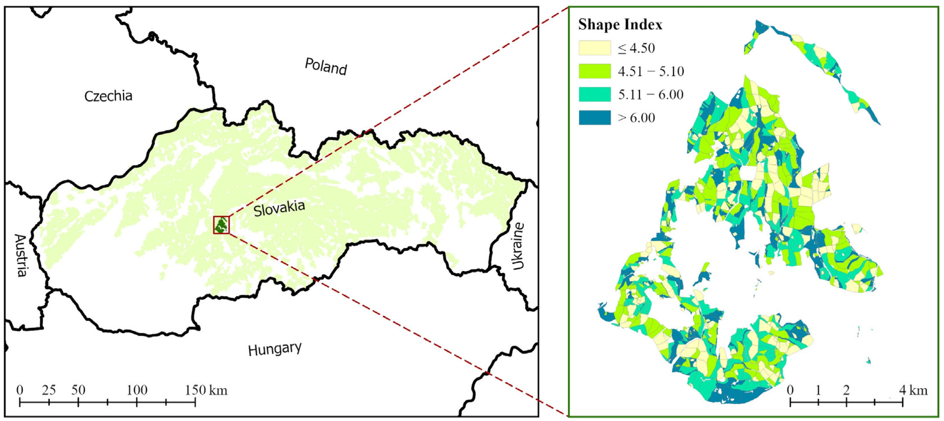
The procedures for generating simulation plots were evaluated using data from the University Forest Enterprise of the Technical University in Zvolen. The University Forest Enterprise is a 9724 ha teaching and research forest situated in central Slovakia (Figure 2). It extends across the Kremnické, Štiavnické, and Javorie mountain ranges—volcanic Carpathian hills rising from approximately 250 m to 1025 m a.s.l. Forest cover is predominantly broadleaved (approximately 85% of the total area), dominated by European beech (Fagus sylvatica L.), with admixtures of oak (Quercus spp.) and hornbeam (Carpinus betulus L.). Coniferous species occupy about 15% of the area, primarily Norway spruce (Picea abies L.) [54]. The forest stand layer utilized in this study was provided by the Institute of Forest Resources and Informatics at the National Forest Centre in Zvolen [55].
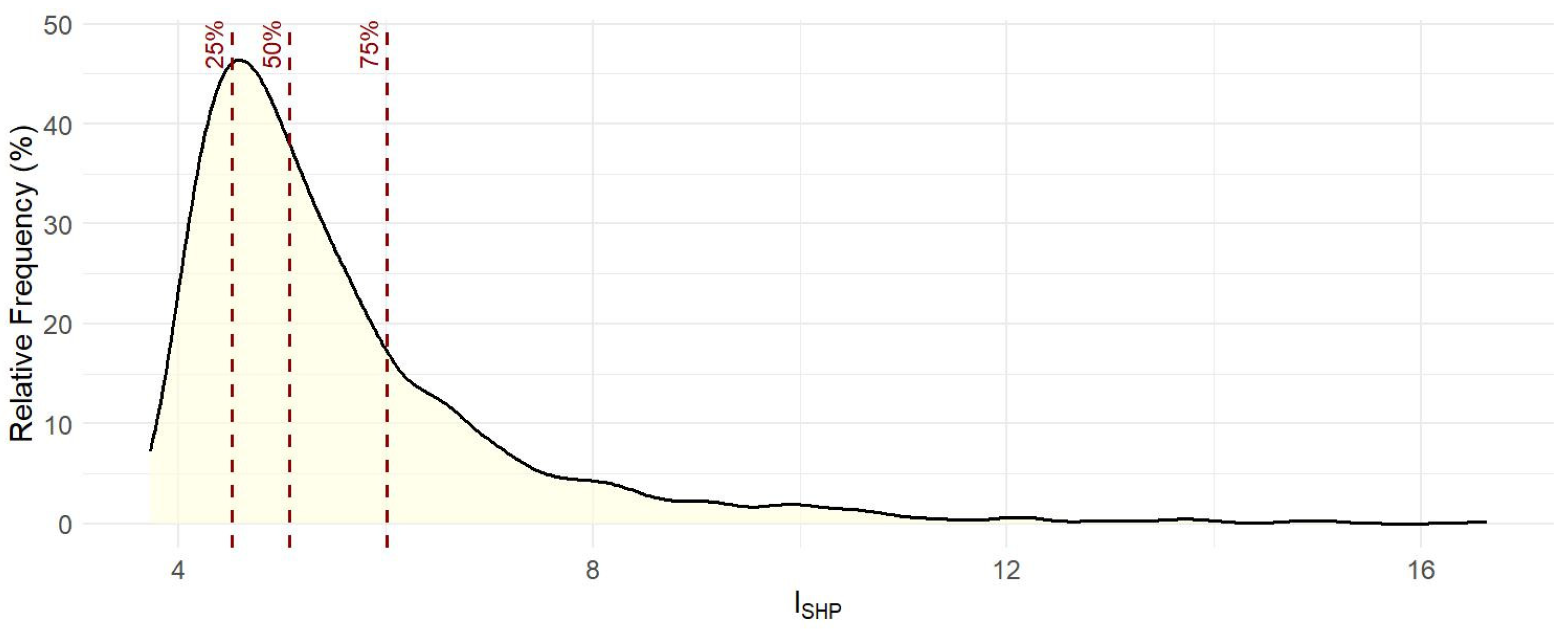
In some instances, forest stands were composed of multiple polygons separated by natural features such as rivers. A total of 983 polygons were retained to comprehensively assess the effectiveness of the simulation plot generation methods, particularly their applicability to a diverse array of forest stand geometries, including less common and highly irregular shapes. As shown in Figure 3, the shapes of the input forest stands ranged from nearly circular polygons ( I S H P = 3.7 ) to highly elongated geometries ( I S H P = 16.6 ). Notably, 90% of the forest stands had a shape index value below 7.5, indicating that relatively compact forms predominated in the evaluation dataset.

3. Results

3.1. Hyperparameter Tuning

Hyperparameter tuning was conducted in parallel on a 12-core processor over approximately three days (73.5 h). Each hyperparameter tuning process was executed as a separate task, resulting in a cumulative processing time of 881.6 h across all 12 processes. In total, 6231 experiments were performed, each involving different randomly selected hyperparameters applied to the input forest stands layer. The extent of the hyperparameter search space is presented in Table 1. Upon completion, performance metrics were imported from a CSV file into R for subsequent statistical analysis [56].
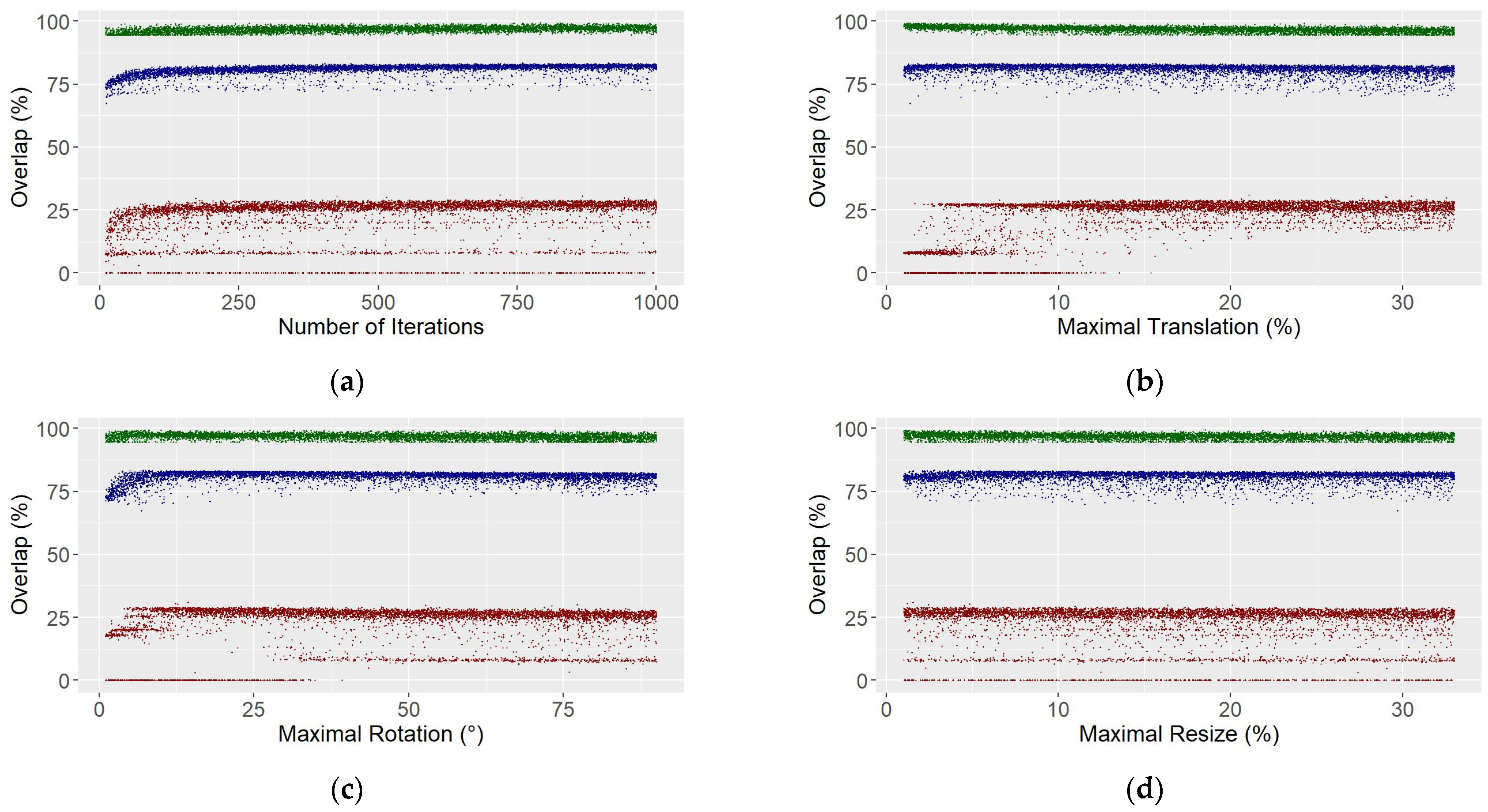
As shown in Figure 4a, a higher number of iterations generally led to a higher overlap percentage. However, increasing the number of iterations did not guarantee non-zero overlap for all simulation plots with the forest stand polygons. Larger values for maximum translation (Figure 4b) and maximum rotation angle (Figure 4c) were associated with improvements in minimum overlap. Allowing a higher resize limit (Figure 4d) resulted in a modest additional increase in overall overlap.
A simulation plot is expected to represent local environmental conditions as closely as possible, thereby providing a robust and accurate framework for modeling forest growth and related processes. Hence, the hyperparameters in the Monte Carlo optimization procedure should be configured to maximize the mean overlap of simulation plots while minimizing the number of plots exhibiting zero or minimal overlap.
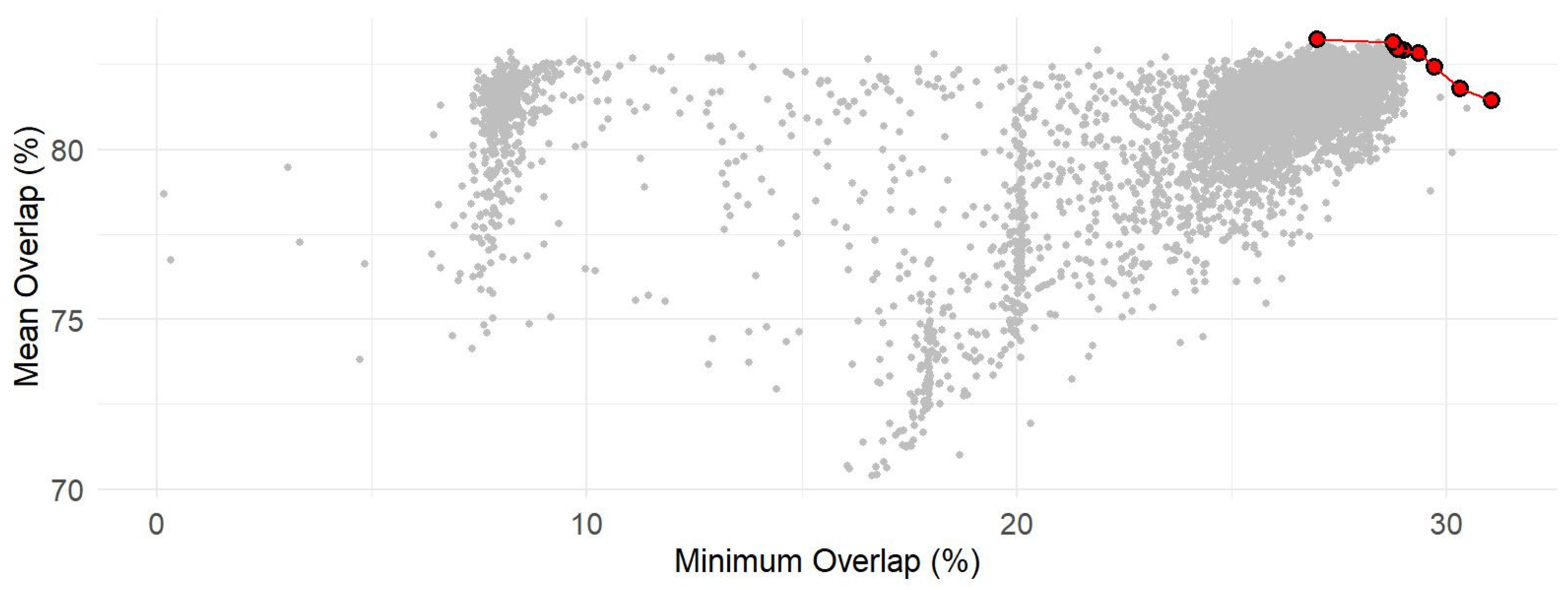
A total of 5711 random hyperparameter configurations resulted in all simulation plots achieving non-zero overlap. A multi-objective optimization approach was used to identify Pareto-optimal configurations that jointly maximize minimum and mean overlap across the plots (Figure 5). These solutions narrowed the acceptable ranges for hyperparameter values (Table 2).
Hyperparameter tuning provided important insights into the sensitivity of the optimization process and revealed ranges of hyperparameter values that produced satisfactory results. Rather than identifying a single optimal configuration, the Pareto frontier yielded multiple acceptable trade-offs between minimum overlap, mean overlap, and computational effort (Table 2). The selection of default values for subsequent analyses therefore accounted for three main factors: (i) maximizing both minimum and mean overlap between simulation plots and forest stands, (ii) maintaining reasonable computing time, and (iii) minimizing the likelihood of convergence to local optima.
Higher values of maximum translation, rotation, and resizing expanded the search space and improved the ability to explore diverse candidate solutions. However, broader ranges also required larger numbers of iterations for fine-tuning and increased computation time. To balance these effects, the maximum random translation, rotation, and resizing were set approximately to the median values observed among the Pareto-optimal configurations (Table 3). This approach provided sufficient flexibility to avoid convergence on local maxima while allowing effective refinement of simulation plot orientation and position. At the same time, the number of iterations was set slightly lower to maintain reasonable computational time without sacrificing the accuracy of plot placement and geometry.
Based on these considerations, and consistent with the outcomes of the Pareto analysis, the default hyperparameter values were set to 800 iterations, 15% maximum translation, 15° maximum rotation, and 5% maximum resize. These values were subsequently applied in the construction of optimized simulation plots for all supported geometric shapes.

3.2. Performance of Optimized Simulation Plots

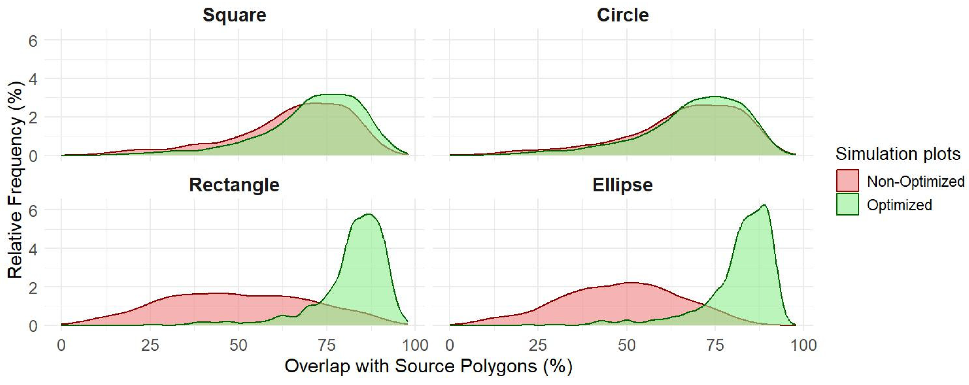
Using the default hyperparameter values derived from the Pareto analysis, optimized simulation plots were produced for all supported geometric shapes. Under these conditions, every optimized plot achieved a non-zero spatial overlap with its corresponding source polygon (Table 4). Rectangular and elliptical plots exhibited notably higher mean overlap values due to their greater adaptability to elongated forest stands. Importantly, the minimum overlap values also increased substantially, particularly for rectangular and elliptical plots, reflecting the effectiveness of the optimization process in reducing poor-fitting configurations.
As shown in Figure 6, the Monte Carlo optimization process was more effective for rectangular and elliptical simulation plots than for square and circular ones. Improper orientation of rectangles and ellipses frequently resulted in very low, or even zero, overlap with the corresponding source polygons. Owing to their asymmetry, these plot shapes benefited substantially from rotation, which improved alignment with the geometry of the source polygons. By contrast, rotation had no effect on symmetric square and circular plots. The combined application of rotation, translation, and resizing to rectangular and elliptical plots led to marked increases in minimum, maximum, and mean overlap with source polygons, as demonstrated in Table 4.
Square and circular simulation plots are inherently limited in their ability to conform to the geometry of elongated source polygons. Their symmetrical shapes restrict flexibility, particularly when polygons exhibit high shape index values or strongly elongated forms. Consequently, optimization of their placement using the Monte Carlo method produced only marginal improvements in spatial overlap across polygons of diverse geometries (Figure 7). Rectangular and elliptical simulation plots, however, showed a much greater capacity to accommodate polygon elongation. When optimized with the Monte Carlo method, these geometries consistently achieved substantial increases in overlap with source polygons across the full range of shape index values. This improvement reflects their ability to adjust aspect ratios and orientations, thereby capturing structural variability and boundary complexity more effectively than square or circular plots. More accurate representation of elongated stands is particularly important for modeling ecological processes such as edge effects, species competition, and resource distribution, thereby enhancing the ecological validity of simulation outcomes.
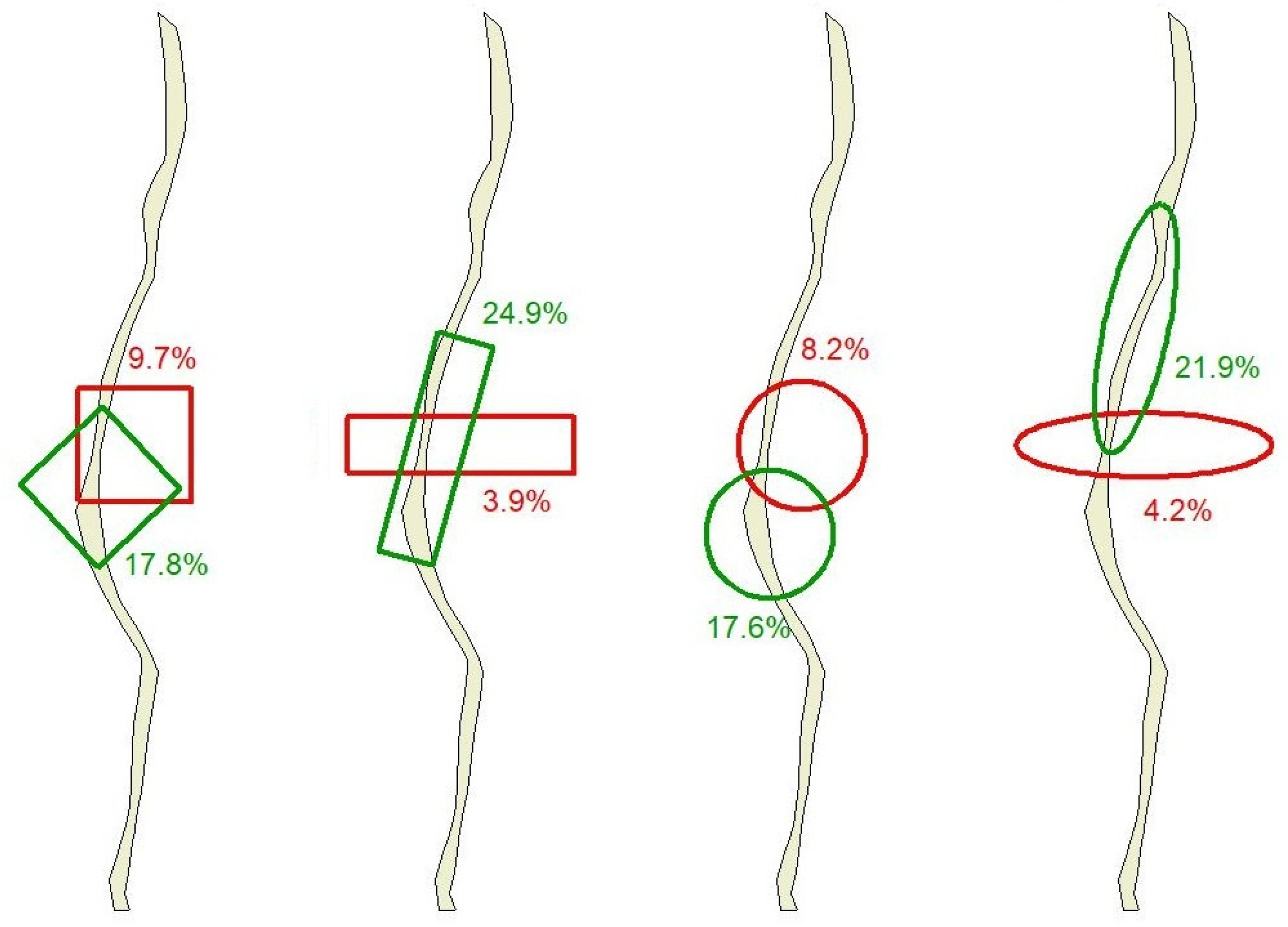
Highly elongated polygons were relatively uncommon, representing only a small fraction of the input dataset (Figure 3). Elongated polygons often represent rare forest ecosystems such as riparian zones, wetland margins, or narrow forest corridors, making accurate simulation plot generation essential for their conservation and management. A total of 29 polygons had a shape index ( I S H P ) greater than 10, accounting for approximately 3% of all polygons. Their areas ranged from 106 m2 to 2.7 ha. These cases are particularly important for evaluating algorithm performance, as regular shapes such as rectangles or ellipses are challenging to adapt to strongly elongated forms. The accuracy of the generated simulation plots for these stands was visually inspected, since improper placement may indicate insufficient optimization. Figure 8 presents an example of the most elongated polygon in the input dataset, fitted with all supported plot shapes.
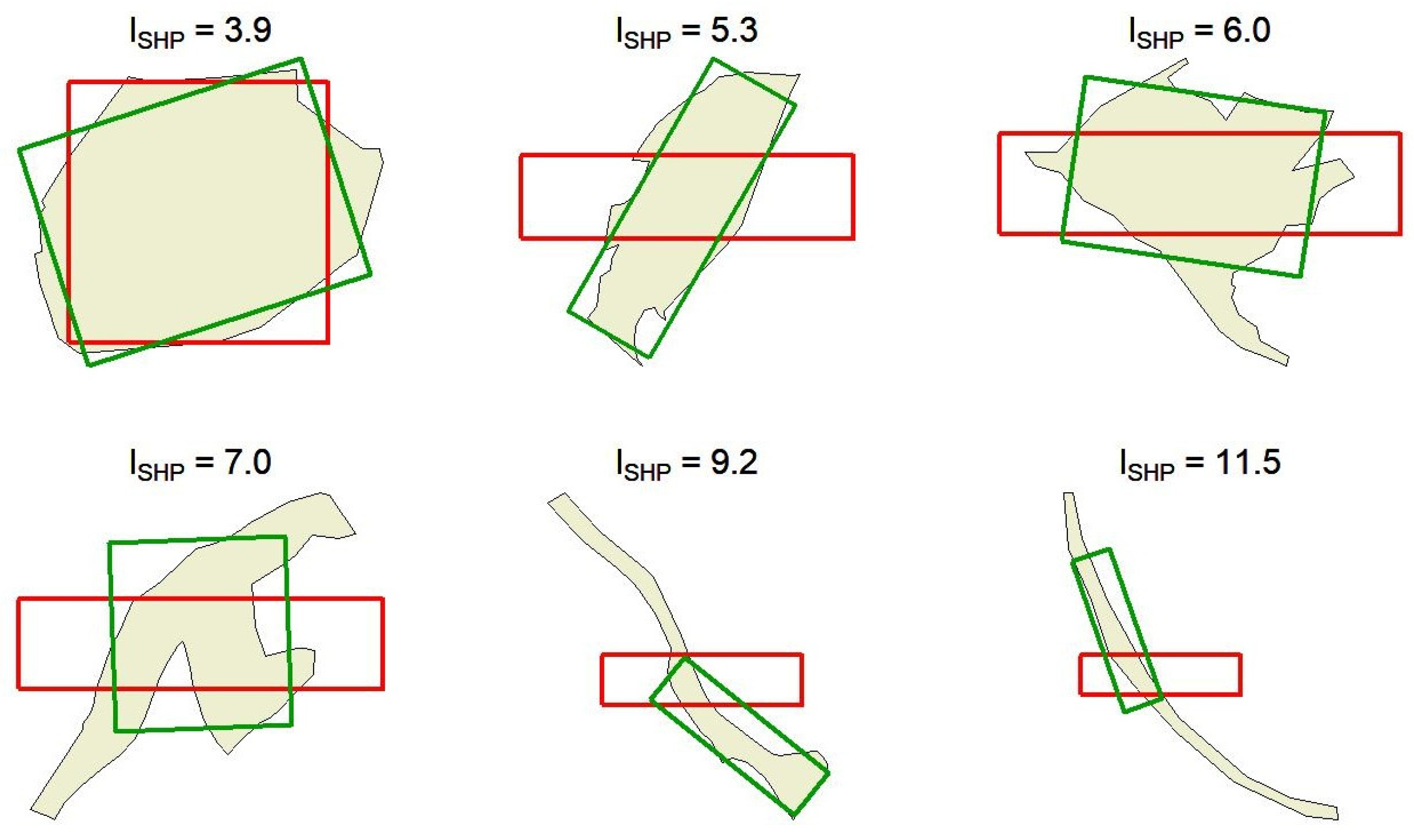
Figure 8 and Figure 9 provide direct before–after visual comparisons of simulation plots. In Figure 8, square, circular, rectangular, and elliptical plots are displayed in both non-optimized and optimized configurations for a highly elongated stand, clearly demonstrating the improvement achieved through optimization. Similarly, Figure 9 illustrates rectangular plots fitted to forest stands with different shape indices, again contrasting initial placements with their optimized counterparts. These overlays emphasize that Monte Carlo refinement substantially increases spatial congruence and enhances the ecological representativeness of simulation plots compared with default placement.

4. Discussion

4.1. Methodological and Practical Contributions

This study advances geoinformatics and forest growth modeling by introducing a Monte Carlo-based optimization framework for generating simulation plots. The approach addresses the challenge of aligning geometric plots with irregular forest management units while preserving ecological representativeness. Although simple shapes such as squares or circles are easy to generate in GIS, their initial placement often leads to biased coverage. Monte Carlo optimization offers a robust alternative by systematically exploring randomized configurations of translations, rotations, and dimensional scaling. This stochastic search enables the identification of configurations with maximum overlap between simulation plots and source polygons, effectively handling the irregular and nonconvex geometries typical of forest stands where deterministic methods often fail.
The integration of hyperparameter tuning further strengthens the method by allowing systematic adjustment of key parameters, ensuring reliable performance across heterogeneous landscapes. Together, these features highlight the potential of Monte Carlo techniques to improve the ecological realism and reliability of forest growth simulations while remaining computationally feasible.
The framework also has practical significance. Optimized simulation plots provide stronger foundations for forest growth models, which are widely used to test management strategies, simulate ecological processes, and assess long-term sustainability. Applications include conservation planning, precision forestry, and agroforestry, where capturing stand-level variability is essential. The adaptability of the Monte Carlo framework also makes it relevant for broader geoinformatics applications, such as land-use modeling, environmental assessment, and spatial decision support systems.
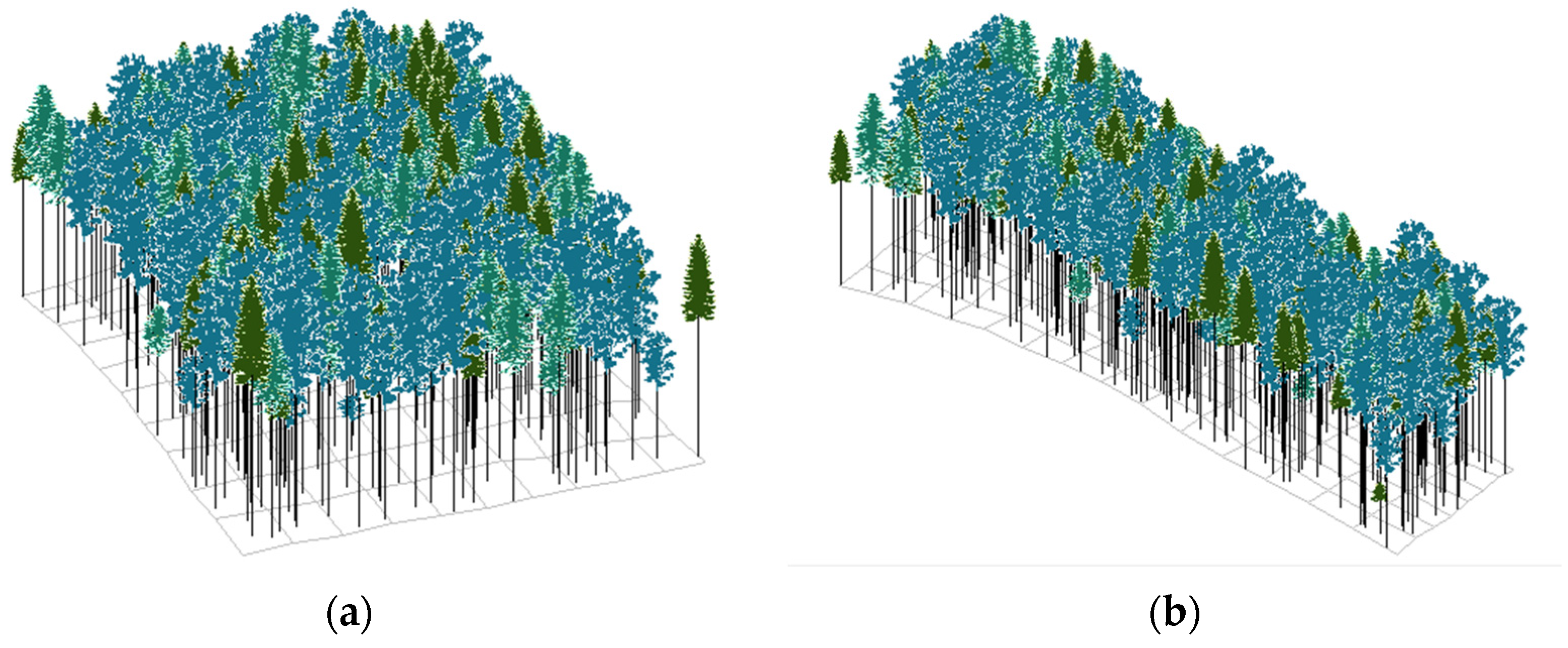
The GenSimPlot QGIS plugin operationalizes this framework, accelerating the preparation of input data and enabling new research on how simulation plot geometry influences modeling outcomes. Figure 10 exemplifies forest growth simulations conducted using the SIBYLA program [27,29] on two differently shaped simulation plots representing an identical forest stand. By modifying plot shape and dimensions, researchers gain insights into how spatial geometry influences ecological interactions and forest stand development. This approach enhances the ecological realism and predictive capacity of forest growth simulations, particularly for stands exhibiting irregular geometries or elongated shapes, which commonly represent ecologically valuable habitats such as riparian forests or wetland ecosystems.
Moreover, optimized simulation plots facilitate investigations into how spatial configuration affects tree competition, light penetration patterns, nutrient cycling, and energy transfers within forest ecosystems. Understanding these spatially dependent processes is crucial for developing management strategies tailored to specific ecological contexts and ensuring long-term forest resilience [57,58,59]. Such insights are critical for improving the ecological realism and predictive power of forest growth models. These functionalities also facilitate forest management in protected areas and examining ecosystem services [60,61], underscoring the plugin’s broad utility for researchers and practitioners alike.
As an open-source QGIS plugin, GenSimPlot provides a robust foundation for developing spatially explicit models across diverse research and management contexts [62,63]. By providing automated tools for generating and optimizing simulation plots, the plugin expands the capacity to simulate crop growth, refine planting configurations, assess fertilizer impacts, and investigate climate change scenarios. Its synergy with QGIS further supports decision-making in conservation agriculture, precision farming, and sustainable intensification [64,65]. In addition, GenSimPlot aids in designing integrated agroforestry systems, conceptualizing urban green spaces, optimizing tree placement, and evaluating environmental impacts [66,67,68].
Beyond forestry applications, the versatility of the GenSimPlot plugin extends to a wide range of research and management domains. Its flexible design allows researchers and practitioners to tailor simulations to meet their unique requirements, promoting sustainable practices and informed decision-making. Potential applications include the assessment of land-use strategies, evaluation of environmental conditions in forest stands, and modeling within agricultural and agroforestry systems.

4.2. Limitations and Future Directions

This study deliberately employed a simple Monte Carlo framework for simulation plot optimization. While the approach provides a flexible and effective means of improving the spatial congruence of simulation plots with source polygons, several limitations should be acknowledged. The method is inherently stochastic, meaning that results may vary between runs even when identical parameter settings are used. Although repeated iterations mitigate this variability, the probabilistic nature of the method can make exact reproducibility more difficult than in deterministic approaches. The optimization process can also be computationally demanding, particularly for large datasets or very high iteration counts. Parallel processing can alleviate some of these demands, but runtime remains a practical consideration in operational contexts.
The framework does not incorporate advanced mechanisms such as adaptive constraint learning, nonlinear weighting, or specialized angle-search schemes, which have been applied in other optimization studies. Future research should explore the integration of these methods and compare their performance with Monte Carlo-based optimization to evaluate potential gains in efficiency and accuracy.
Another limitation lies in handling very irregular and highly elongated polygons. In the optimization process, the maximum side ratio for bounding boxes was constrained to a value of four. This restriction was introduced to prevent the generation of excessively long and narrow plots, which may be ecologically unrealistic and unsuitable for modeling applications. While this constraint improves ecological plausibility and computational stability, it also limits the adaptability of simulation plots to highly elongated polygons. Increasing the allowable side ratio could, in principle, enhance spatial overlap with extreme polygon geometries. However, such adjustments risk reducing the ecological representativeness of simulation plots by exaggerating edge effects and compromising their ability to capture stand-level dynamics in a balanced manner.
Although highly elongated polygons constituted only a small portion of the input dataset, they are ecologically important, often corresponding to rare and valuable forest ecosystems such as riparian zones, wetland margins, narrow corridors along slopes, ravines, and linear remnants of natural vegetation. Accurate simulation plot generation for such stands is therefore particularly critical. Broader testing with larger and more diverse datasets will provide further insights and improvements, especially in refining initial placement, rotation, and resizing strategies for simulation plots.
The current implementation offers several options for initial plot placement, but these are deterministic and simulation plot placement can become trapped in local maxima. Alternative strategies could involve random initialization within the source polygon or stratified placement along its longest axis. Another promising approach is to position the plot at the internal point with the maximum distance from the polygon boundary, corresponding to the deepest interior location.
Rotation of simulation plot geometries may also be improved. Deterministic exploration can be achieved by systematically rotating the geometry at a given location, while principal component analysis (PCA) can be used to identify the main axis of the polygon, thereby informing both the optimal rotation angle and the initial placement.
The method also inherits limitations related to hyperparameter selection. Although tuning improves performance, optimal parameter values may vary across datasets, and their transferability remains uncertain. Alternative approaches, such as Bayesian optimization, could be explored to enhance robustness.
Validation in this study was performed using geometric overlap metrics, which provide a clear and reproducible measure of spatial congruence but do not directly capture ecological processes or species-specific dynamics. We acknowledge that ecological validation—linking plot geometry to derived biophysical variables such as soil moisture, light availability, or species composition—would provide stronger evidence of practical applicability. Incorporating ecological indicators into the evaluation would therefore enhance confidence in the representativeness of optimized plots. The GenSimPlot plugin has been explicitly designed to facilitate such analyses, for example by extracting terrain and environmental variables within simulation plots. However, comprehensive ecological validation will require integration with forest growth simulators and the use of extensive experimental datasets.
While this study demonstrates the effectiveness of Monte Carlo-based optimization for improving the spatial congruence of simulation plots with source polygons, an important limitation is the absence of direct comparison with alternative optimization techniques. Systematic benchmarking against methods such as gradient-based optimization, simulated annealing, or genetic algorithms was not included, as such work would require substantial development, integration of external libraries, parameter calibration, and dedicated benchmarking protocols. Although beyond the scope of this study, comparative analyses represent a promising direction for future research and would provide practical guidance for selecting appropriate optimization strategies in geoinformatics and forestry applications.
Alternative approaches each offer distinct advantages and limitations. Gradient-based optimization can converge rapidly when objective functions are smooth and well-behaved, but it performs poorly with irregular and nonconvex polygon geometries where local optima are frequent. Simulated annealing, a probabilistic method that accepts inferior solutions during early search phases, has been applied successfully in forestry tasks such as harvest planning and cableway layout design [69,70]. Its performance, however, depends strongly on the cooling schedule and algorithmic parameters. Genetic algorithms, inspired by evolutionary processes, employ selection, crossover, and mutation to explore solution spaces. They have proven effective for multi-objective forest management and spatial optimization problems [71,72,73], but require extensive parameterization, computational resources, and integration of specialized libraries.
Compared with these deterministic and metaheuristic alternatives, the Monte Carlo approach adopted here emphasizes transparency and simplicity. It avoids complex parameterization, employs a compact hyperparameter-tuning workflow, and remains computationally tractable across heterogeneous landscapes. Although other methods may converge more rapidly under favorable conditions, their reliance on sensitive parameters can hinder reproducibility and adoption. In this respect, Monte Carlo optimization provides a robust and accessible baseline while motivating future research on hybrid strategies that combine adaptive search mechanisms with transparent implementation.
Future work should include systematic comparative evaluations of Monte Carlo and alternative optimization methods across a range of forest stand complexities and data conditions. Such analyses would clarify the relative strengths of each approach and provide practical guidance for selecting optimization strategies suited to different ecological and computational contexts.
Despite these limitations, the Monte Carlo-based framework presented herein offers a robust foundation for applications in forest growth modeling, agroforestry planning, and landscape-scale climate assessments. Further development through rigorous benchmarking, computational refinements, and ecological validation will enhance its reliability, broaden its generalizability, and increase its utility in real-world geoinformatics and decision-support applications.

5. Conclusions

This study demonstrates that Monte Carlo-based optimization offers a robust and effective approach for refining the spatial alignment, orientation, and geometry of simulation plots in heterogeneous forest stands. By systematically exploring candidate configurations through iterative random sampling, the method improves spatial congruence between simulation plots and their corresponding forest stands. Combined with simple geometric shapes (square, circle, rectangle, and ellipse), the approach increases adaptability to diverse stand geometries. Rectangular and elliptical plots, in particular, provide greater flexibility for elongated or irregular stands, thereby enhancing ecological representativeness in forest growth simulations. Integrated hyperparameter tuning further enables users to balance optimization quality with computational efficiency, strengthening robustness across datasets.
The workflow is complemented by environmental variable extraction within a GIS environment, providing essential inputs for scenario-based analyses in forestry, agroforestry, and conservation agriculture. Implemented as an open-source QGIS plugin, the framework facilitates transparent, reproducible, and readily deployable spatial modeling.
We acknowledge several limitations, including the computational cost of large-scale applications, stochastic variability across runs, and the need for broader validation beyond the study region. Future work will focus on scalable computational strategies, benchmarking against alternative optimization methods, and ecological validation through integration with growth simulators and independent field or remote sensing data. Applying the framework to additional spatial datasets and biophysical parameters—and validating it across other domains that require precise, spatially explicit modeling—will further strengthen its generality and practical impact.

Author Contributions

Conceptualization, Milan Koreň; methodology, Milan Koreň and Marek Fabrika; software, Milan Koreň and Peter Márton; investigation, Milan Koreň and Marek Fabrika; writing—original draft preparation, Milan Koreň; writing—review and editing, Milan Koreň, Peter Márton, Mosab Khalil Algidail Arbain, Peter Valent, Roman Sitko, and Marek Fabrika; visualization, Milan Koreň and Peter Valent; funding acquisition, Roman Sitko. All authors have read and agreed to the published version of the manuscript.

Funding

This work was supported by the project Research on the Application of Artificial Intelligence Tools in the Analysis and Classification of Hyperspectral Sensing Data (HYSPED), ITMS 313011BWC9, under the Operational Program Integrated Infrastructure (OPII) funded by the European Regional Development Fund (ERDF), and the NextGenerationEU instrument through the Recovery and Resilience Plan for Slovakia (Project No. 09I03-03-V02-00034).

Data Availability Statement

The data presented in this study are available from the corresponding author upon reasonable request.

Conflicts of Interest

The authors declare no conflicts of interest.

References

  1. Blanco, J.A.; Lo, Y.-H. Latest Trends in Modelling Forest Ecosystems: New Approaches or Just New Methods? Curr. For. Rep. 2023, 9, 219–229. [Google Scholar] [CrossRef]
  2. Maréchaux, I.; Langerwisch, F.; Huth, A.; Bugmann, H.; Morin, X.; Reyer, C.P.O.; Seidl, R.; Collalti, A.; Dantas De Paula, M.; Fischer, R.; et al. Tackling Unresolved Questions in Forest Ecology: The Past and Future Role of Simulation Models. Ecol. Evol. 2021, 11, 3746–3770. [Google Scholar] [CrossRef] [PubMed]
  3. Mahnken, M.; Cailleret, M.; Collalti, A.; Trotta, C.; Biondo, C.; D’Andrea, E.; Dalmonech, D.; Marano, G.; Mäkelä, A.; Minunno, F.; et al. Accuracy, Realism and General Applicability of European Forest Models. Glob. Change Biol. 2022, 28, 6921–6943. [Google Scholar] [CrossRef] [PubMed]
  4. Boukhris, I.; Marano, G.; Dalmonech, D.; Valentini, R.; Collalti, A. Modeling Forest Growth Under Current and Future Climate. Curr. For. Rep. 2025, 11, 17. [Google Scholar] [CrossRef]
  5. Grünig, M.; Rammer, W.; Albrich, K.; André, F.; Augustynczik, A.L.D.; Bohn, F.; Bouwman, M.; Bugmann, H.; Collalti, A.; Cristal, I.; et al. A Harmonized Database of European Forest Simulations Under Climate Change. Data Brief 2024, 54, 110384. [Google Scholar] [CrossRef]
  6. Rammer, W.; Thom, D.; Baumann, M.; Braziunas, K.; Dollinger, C.; Kerber, J.; Mohr, J.; Seidl, R. The Individual-Based Forest Landscape and Disturbance Model iLand: Overview, Progress, and Outlook. Ecol. Model. 2024, 495, 110785. [Google Scholar] [CrossRef]
  7. Gao, Y.; Li, L.; Du, X.; Meng, J. A Transition-Matrix Growth Model and Equilibrium Curve for Natural Forests in Jiangxi Province. Forests 2023, 14, 2038. [Google Scholar] [CrossRef]
  8. Lei, K.; Zhang, H.; Qiu, H.; Yang, T.; Liu, Y.; Zhang, J.; Hu, X.; Cui, Z. A Novel Strategy for Constructing Large-Scale Forest Scene: Integrating Forest Hierarchical Models and Tree Growth Models to Improve the Efficiency and Stability of Forest Polymorphism Simulation. Forests 2023, 14, 1595. [Google Scholar] [CrossRef]
  9. Giebink, C.L.; DeRose, R.J.; Castle, M.; Shaw, J.D.; Evans, M.E.K. Climatic Sensitivities Derived from Tree Rings Improve Predictions of the Forest Vegetation Simulator Growth and Yield Model. For. Ecol. Manag. 2022, 517, 120256. [Google Scholar] [CrossRef]
  10. Pukkala, T.; Vauhkonen, J.; Korhonen, K.T.; Packalen, T. Self-Learning Growth Simulator for Modelling Forest Stand Dynamics in Changing Conditions. For. Int. J. For. Res. 2021, 94, 333–346. [Google Scholar] [CrossRef]
  11. Pretzsch, H. The Course of Tree Growth. Theory and Reality. For. Ecol. Manag. 2020, 478, 118508. [Google Scholar] [CrossRef]
  12. Liu, C.; Calders, K.; Origo, N.; Disney, M.; Meunier, F.; Woodgate, W.; Gastellu-Etchegorry, J.-P.; Nightingale, J.; Honkavaara, E.; Hakala, T.; et al. Reconstructing the Digital Twin of Forests from a 3D Library: Quantifying Trade-Offs for Radiative Transfer Modeling. Remote Sens. Environ. 2023, 298, 113832. [Google Scholar] [CrossRef]
  13. Toba, A.-L.; Paudel, R.; Davis, C.; Hartley, D.S.; Gandhi Mendadhala, R.V. ITreeForeCast: An Integrated Modeling Software to Simulate Tree Level Growth and Forest Carbon Storage. Comput. Electron. Agric. 2025, 237, 110495. [Google Scholar] [CrossRef]
  14. Schauberger, B.; Jägermeyr, J.; Gornott, C. A Systematic Review of Local to Regional Yield Forecasting Approaches and Frequently Used Data Resources. Eur. J. Agron. 2020, 120, 126153. [Google Scholar] [CrossRef]
  15. Paudel, D.; Boogaard, H.; De Wit, A.; Janssen, S.; Osinga, S.; Pylianidis, C.; Athanasiadis, I.N. Machine Learning for Large-Scale Crop Yield Forecasting. Agric. Syst. 2021, 187, 103016. [Google Scholar] [CrossRef]
  16. Dlamini, L.; Crespo, O.; Van Dam, J.; Kooistra, L. A Global Systematic Review of Improving Crop Model Estimations by Assimilating Remote Sensing Data: Implications for Small-Scale Agricultural Systems. Remote Sens. 2023, 15, 4066. [Google Scholar] [CrossRef]
  17. Xu, X.; Gao, F.; Xiong, D.; Fan, Z.; Xiong, S.; Dong, P.; Qiao, H.; Ma, X. Digital Twin-Based Winter Wheat Growth Simulation and Optimization. Field Crops Res. 2025, 329, 109953. [Google Scholar] [CrossRef]
  18. Gejdoš, M.; Michajlová, K. Analysis of Current and Future Forest Disturbances Dynamics in Central Europe. Forests 2022, 13, 554. [Google Scholar] [CrossRef]
  19. Bošeľa, M.; Petráš, R.; Šebeň, V.; Mecko, J.; Marušák, R. Evaluating Competitive Interactions between Trees in Mixed Forests in the Western Carpathians: Comparison Between Long-Term Experiments and SIBYLA Simulations. For. Ecol. Manag. 2013, 310, 577–588. [Google Scholar] [CrossRef]
  20. Irauschek, F.; Barka, I.; Bugmann, H.; Courbaud, B.; Elkin, C.; Hlásny, T.; Klopcic, M.; Mina, M.; Rammer, W.; Lexer, M.J. Evaluating Five Forest Models Using Multi-Decadal Inventory Data from Mountain Forests. Ecol. Model. 2021, 445, 109493. [Google Scholar] [CrossRef]
  21. Hlásny, T.; Barcza, Z.; Barka, I.; Merganičová, K.; Sedmák, R.; Kern, A.; Pajtík, J.; Balázs, B.; Fabrika, M.; Churkina, G. Future Carbon Cycle in Mountain Spruce Forests of Central Europe: Modelling Framework and Ecological Inferences. For. Ecol. Manag. 2014, 328, 55–68. [Google Scholar] [CrossRef]
  22. Hansen, J.W.; Jones, J.W. Scaling-up Crop Models for Climate Variability Applications. Agric. Syst. 2000, 65, 43–72. [Google Scholar] [CrossRef]
  23. Nabhani, A.; Sjølie, H.K. TreeSim: An Object-Oriented Individual Tree Simulator and 3D Visualization Tool in Python. SoftwareX 2022, 20, 101221. [Google Scholar] [CrossRef]
  24. Wimmler, M.-C.; Bathmann, J.; Vollhüter, J.; Berger, U. pyMANGA: A Modular, Open and Extendable Software Platform for Modeling of Forest and Vegetation Dynamics. Environ. Model. Softw. 2024, 174, 105973. [Google Scholar] [CrossRef]
  25. Bravo, F.; Ordóñez, C.; Vázquez-Veloso, A.; Michalakopoulos, S. SIMANFOR Cloud Decision Support System: Structure, Content, and Applications. Ecol. Model. 2025, 499, 110912. [Google Scholar] [CrossRef]
  26. Thurnher, C.; Klopf, M.; Hasenauer, H. MOSES—A Tree Growth Simulator for Modelling Stand Response in Central Europe. Ecol. Model. 2017, 352, 58–76. [Google Scholar] [CrossRef]
  27. Fabrika, M.; Ďurský, J. Algorithms and Software Solution of Thinning Models for SIBYLA Growth Simulator. J. For. Sci. 2005, 51, 431–445. [Google Scholar] [CrossRef]
  28. Machar, I.; Simon, J.; Brus, J.; Pechanec, V.; Kiliánová, H.; Filippovová, J.; Vrublová, K.; Mackovcin, P. A Growth Simulation Model as a Support Tool for Conservation Management Strategy in a Mountain Protected Area. eco.mont 2018, 10, 61–69. [Google Scholar] [CrossRef]
  29. Fabrika, M.; Valent, P.; Scheer, Ľ. Thinning Trainer Based on Forest-Growth Model, Virtual Reality and Computer-Aided Virtual Environment. Environ. Model. Softw. 2018, 100, 11–23. [Google Scholar] [CrossRef]
  30. Ma, Z.; Chen, M.; Zhang, B.; Wang, M.; Shen, C.; Yue, S.; Wen, Y.; Lü, G. A Web-Based Integrated Modeling and Simulation Method for Forest Growth Research. Earth Space Sci. 2019, 6, 2142–2159. [Google Scholar] [CrossRef]
  31. Liu, Y.; Tang, W.; He, J.; Liu, Y.; Ai, T.; Liu, D. A Land-Use Spatial Optimization Model Based on Genetic Optimization and Game Theory. Comput. Environ. Urban Syst. 2015, 49, 1–14. [Google Scholar] [CrossRef]
  32. Baskent, E.Z.; Borges, J.G.; Kašpar, J. An Updated Review of Spatial Forest Planning: Approaches, Techniques, Challenges, and Future Directions. Curr. For. Rep. 2024, 10, 299–321. [Google Scholar] [CrossRef]
  33. Dong, L.; Bettinger, P.; Liu, Z.; Qin, H.; Zhao, Y. Evaluating the Neighborhood, Hybrid and Reversion Search Techniques of a Simulated Annealing Algorithm in Solving Forest Spatial Harvest Scheduling Problems. Silva Fenn. 2016, 50, 1622. [Google Scholar] [CrossRef]
  34. Mrkvička, T.; Soubeyrand, S.; Myllymäki, M.; Grabarnik, P.; Hahn, U. Monte Carlo Testing in Spatial Statistics, with Applications to Spatial Residuals. Spat. Stat. 2016, 18, 40–53. [Google Scholar] [CrossRef]
  35. Goodbody, T.R.H.; Coops, N.C.; Senf, C.; Seidl, R. Airborne Laser Scanning to Optimize the Sampling Efficiency of a Forest Management Inventory in South-Eastern Germany. Ecol. Indic. 2023, 157, 111281. [Google Scholar] [CrossRef]
  36. Rodríguez-Ruiz, J.; Martínez-Calvo, A.; Pérez-Cruzado, C. Designing Circular Fixed-Area Plots in Large-Scale Forest Inventories: Effect of Horizontal Distance Measurement Uncertainty and Tree Position Pattern. Can. J. For. Res. 2025, 55, 1–14. [Google Scholar] [CrossRef]
  37. Waeselynck, V.; Saah, D. Importance Sampling for Cost-Optimized Estimation of Burn Probability Maps in Wildfire Monte Carlo Simulations. Fire 2024, 7, 455. [Google Scholar] [CrossRef]
  38. Gomes, V.d.S.; Monti, C.A.U.; Silva, C.S.J.e.; Gomide, L.R. Operational Harvest Planning Under Forest Road Maintenance Uncertainty. For. Policy Econ. 2021, 131, 102562. [Google Scholar] [CrossRef]
  39. Zeng, H.; Garcia-Gonzalo, J.; Peltola, H.; Kellomäki, S. The Effects of Forest Structure on the Risk of Wind Damage at a Landscape Level in a Boreal Forest Ecosystem. Ann. For. Sci. 2010, 67, 111. [Google Scholar] [CrossRef]
  40. Sambakhe, D.; Fortin, M.; Renaud, J.-P.; Deleuze, C.; Dreyfus, P.; Picard, N. Prediction Bias Induced by Plot Size in Forest Growth Models. For. Sci. 2014, 60, 1050–1059. [Google Scholar] [CrossRef]
  41. Pöpperl, F.; Seidl, R. Effects of Stand Edges on the Structure, Functioning, and Diversity of a Temperate Mountain Forest Landscape. Ecosphere 2021, 12, e03692. [Google Scholar] [CrossRef]
  42. Torresani, M.; Montagnani, L.; Rocchini, D.; Moudrý, V.; Andreoli, A.; Wellstein, C.; Koyanagi, K.; Ros, L.D.; Bacaro, G.; Perrone, M.; et al. LiDAR Insights on Stand Structure and Topography in Mountain Forest Wind Extreme Events: The Vaia Case Study. Agric. For. Meteorol. 2024, 359, 110267. [Google Scholar] [CrossRef]
  43. Firmino, P.N.; Tomé, M.; Paulo, J.A. Do Distance-Dependent Competition Indices Contribute to Improve Diameter and Total Height Tree Growth Prediction in Juvenile Cork Oak Plantations? Forests 2023, 14, 1066. [Google Scholar] [CrossRef]
  44. Rieder, J.S.; Link, R.M.; Köthe, K.; Seidel, D.; Ullmann, T.; Žmegač, A.; Zang, C.; Schuldt, B. TreeCompR: Tree Competition Indices for Inventory Data and 3D Point Clouds. Methods Ecol. Evol. 2024, 15, 2198–2208. [Google Scholar] [CrossRef]
  45. Fazlollahi Mohammadi, M.; Tobin, B.; Jalali, S.G.; Kooch, Y.; Riemann, R. Fine-Scale Topographic Influence on the Spatial Distribution of Tree Species Diameter in Old-Growth Beech (Fagus orientalis Lipsky.) Forests, Northern Iran. Sci. Rep. 2022, 12, 7633. [Google Scholar] [CrossRef]
  46. Raigosa-García, I.; Rathbun, L.C.; Cook, R.L.; Baker, J.S.; Corrao, M.V.; Sumnall, M.J. Rethinking Productivity Evaluation in Precision Forestry Through Dominant Height and Site Index Measurements Using Aerial Laser Scanning LiDAR Data. Forests 2024, 15, 1002. [Google Scholar] [CrossRef]
  47. Nunes, M.H.; Jucker, T.; Riutta, T.; Svátek, M.; Kvasnica, J.; Rejžek, M.; Matula, R.; Majalap, N.; Ewers, R.M.; Swinfield, T.; et al. Recovery of Logged Forest Fragments in a Human-Modified Tropical Landscape During the 2015-16 El Niño. Nat. Commun. 2021, 12, 1526. [Google Scholar] [CrossRef]
  48. Fiandino, S.; Plevich, J.; Tarico, J.; Utello, M.; Demaestri, M.; Gyenge, J. Modeling Forest Site Productivity Using Climate Data and Topographic Imagery in Pinus elliottii Plantations of Central Argentina. Ann. For. Sci. 2020, 77, 95. [Google Scholar] [CrossRef]
  49. Li, Q.; Hu, B.; Shang, J.; Remmel, T.K. Two-Stage Deep Learning Framework for Individual Tree Crown Detection and Delineation in Mixed-Wood Forests Using High-Resolution Light Detection and Ranging Data. Remote Sens. 2025, 17, 1578. [Google Scholar] [CrossRef]
  50. Lisiewicz, M.; Kamińska, A.; Kraszewski, B.; Stereńczak, K. Correcting the Results of CHM-Based Individual Tree Detection Algorithms to Improve Their Accuracy and Reliability. Remote Sens. 2022, 14, 1822. [Google Scholar] [CrossRef]
  51. Vanderwel, M.C.; Lopez, E.L.; Sprott, A.H.; Khayyatkhoshnevis, P.; Shovon, T.A. Using Aerial Canopy Data from UAVs to Measure the Effects of Neighbourhood Competition on Individual Tree Growth. For. Ecol. Manag. 2020, 461, 117949. [Google Scholar] [CrossRef]
  52. Holm, S.; Schweier, J. Virtual Forests for Decision Support and Stakeholder Communication. Environ. Model. Softw. 2024, 180, 106159. [Google Scholar] [CrossRef]
  53. Yu, H.; Wu, M.M.; He, H.S. Developing Platform of 3-D Visualization of Forest Landscape. Environ. Model. Softw. 2022, 157, 105524. [Google Scholar] [CrossRef]
  54. Merganič, J.; Merganičová, K.; Vlčková, M.; Dudáková, Z.; Ferenčík, M.; Mokroš, M.; Juško, V.; Allman, M.; Tomčík, D. Deadwood Amount at Disturbance Plots After Sanitary Felling. Plants 2022, 11, 987. [Google Scholar] [CrossRef]
  55. Datasets, National Forest Centre (NLC), Slovakia. Available online: https://web.nlcsk.org/datasety/ (accessed on 5 September 2025).
  56. R Core Team. R: A Language and Environment for Statistical Computing; R Foundation for Statistical Computing: Vienna, Austria, 2021. [Google Scholar]
  57. Kükenbrink, D.; Schneider, F.D.; Schmid, B.; Gastellu-Etchegorry, J.-P.; Schaepman, M.E.; Morsdorf, F. Modelling of Three-Dimensional, Diurnal Light Extinction in Two Contrasting Forests. Agric. For. Meteorol. 2021, 296, 108230. [Google Scholar] [CrossRef]
  58. Meeussen, C.; Govaert, S.; Vanneste, T.; Calders, K.; Bollmann, K.; Brunet, J.; Cousins, S.A.O.; Diekmann, M.; Graae, B.J.; Hedwall, P.-O.; et al. Structural Variation of Forest Edges Across Europe. For. Ecol. Manag. 2020, 462, 117929. [Google Scholar] [CrossRef]
  59. Pang, L.; Wang, G.; Sharma, R.P.; Lu, J.; Tang, X.; Fu, L. Simulation of Thinning by Integrating Tree Competition and Species Biodiversity for Target Tree-Based Management of Secondary Forests. Forests 2023, 14, 1896. [Google Scholar] [CrossRef]
  60. Schmid, U.; Frehner, M.; Glatthorn, J.; Bugmann, H. ProForM: A Simulation Model for the Management of Mountain Protection Forests. Ecol. Model. 2023, 478, 110297. [Google Scholar] [CrossRef]
  61. Ezquerro, M.; Diaz-Balteiro, L.; Pardos, M. Implications of Forest Management on the Conservation of Protected Areas: A New Proposal in Central Spain. For. Ecol. Manag. 2023, 548, 121428. [Google Scholar] [CrossRef]
  62. Langhammer, M.; Thober, J.; Lange, M.; Frank, K.; Grimm, V. Agricultural Landscape Generators for Simulation Models: A Review of Existing Solutions and an Outline of Future Directions. Ecol. Model. 2019, 393, 135–151. [Google Scholar] [CrossRef]
  63. Henniger, H.; Huth, A.; Frank, K.; Bohn, F.J. Creating Virtual Forests around the Globe and Analysing Their State Space. Ecol. Model. 2023, 483, 110404. [Google Scholar] [CrossRef]
  64. Shahhosseini, M.; Hu, G.; Huber, I.; Archontoulis, S.V. Coupling Machine Learning and Crop Modeling Improves Crop Yield Prediction in the US Corn Belt. Sci. Rep. 2021, 11, 1606. [Google Scholar] [CrossRef]
  65. Hernández-Ochoa, I.M.; Gaiser, T.; Kersebaum, K.-C.; Webber, H.; Seidel, S.J.; Grahmann, K.; Ewert, F. Model-Based Design of Crop Diversification Through New Field Arrangements in Spatially Heterogeneous Landscapes. A Review. Agron. Sustain. Dev. 2022, 42, 74. [Google Scholar] [CrossRef]
  66. Jahel, C.; Baron, C.; Vall, E.; Karambiri, M.; Castets, M.; Coulibaly, K.; Bégué, A.; Lo Seen, D. Spatial Modelling of Agro-Ecosystem Dynamics across Scales: A Case in the Cotton Region of West-Burkina Faso. Agric. Syst. 2017, 157, 303–315. [Google Scholar] [CrossRef]
  67. Rahman, M.H.U.; Ahrends, H.E.; Raza, A.; Gaiser, T. Current Approaches for Modeling Ecosystem Services and Biodiversity in Agroforestry Systems: Challenges and Ways Forward. Front. For. Glob. Change 2023, 5, 1032442. [Google Scholar] [CrossRef]
  68. Kraft, P.; Rezaei, E.E.; Breuer, L.; Ewert, F.; Große-Stoltenberg, A.; Kleinebecker, T.; Seserman, D.-M.; Nendel, C. Modelling Agroforestry’s Contributions to People—A Review of Available Models. Agronomy 2021, 11, 2106. [Google Scholar] [CrossRef]
  69. Dong, L.; Bettinger, P.; Liu, Z. Optimizing Neighborhood-Based Stand Spatial Structure: Four Cases of Boreal Forests. For. Ecol. Manag. 2022, 506, 119965. [Google Scholar] [CrossRef]
  70. Retzlaff, C.O.; Gollob, C.; Nothdurft, A.; Stampfer, K.; Holzinger, A. Multi-Objective Optimization of Cable-Road Layouts in Smart Forestry. Int. J. For. Eng. 2024, 35, 444–455. [Google Scholar] [CrossRef] [PubMed]
  71. Castro, I.; Salas-González, R.; Fidalgo, B.; Farinha, J.T.; Mendes, M. Optimising Forest Management Using Multi-Objective Genetic Algorithms. Sustainability 2024, 16, 10655. [Google Scholar] [CrossRef]
  72. Ding, M.; Yin, X.; Pan, S.; Liu, P. Multi-Objective Spatial Optimization of Protective Forests Based on the Non-Dominated Sorting Genetic Algorithm-II Algorithm and Future Land Use Simulation Model: A Case Study of Alaer City, China. Forests 2025, 16, 452. [Google Scholar] [CrossRef]
  73. Fotakis, D.G.; Sidiropoulos, E.; Myronidis, D.; Ioannou, K. Spatial Genetic Algorithm for Multi-Objective Forest Planning. For. Policy Econ. 2012, 21, 12–19. [Google Scholar] [CrossRef]
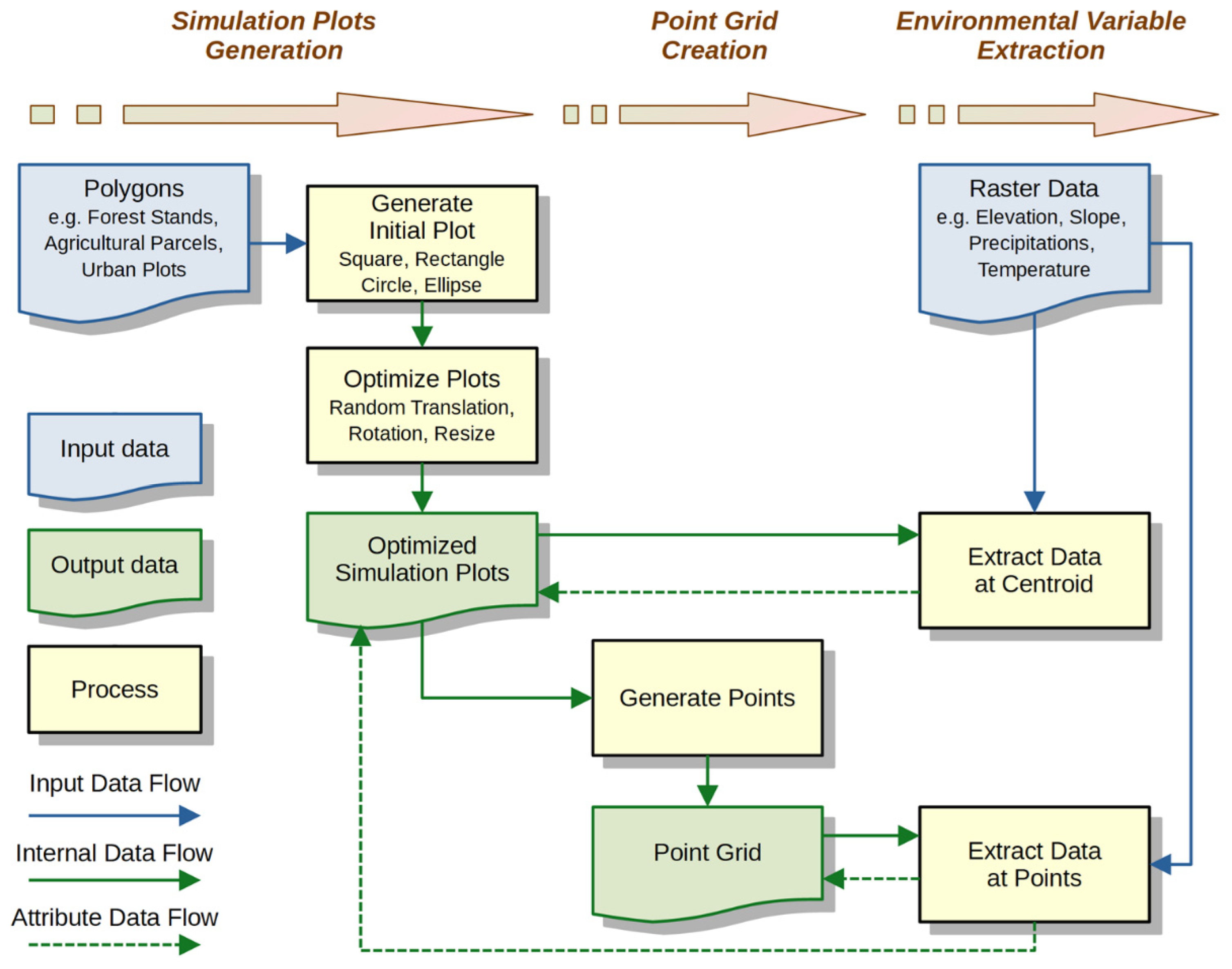
Figure 1. Workflow for generating and optimizing simulation plots, creating a point grid, and extracting environmental variables in GenSimPlot.
Ijgi 14 00408 g001
Figure 2. Location of the research area within Slovakia (left) and spatial distribution of forest stand shape indices (right). Shape index categories correspond to quantiles of the relative frequency distribution.
Ijgi 14 00408 g002
Figure 3. Relative frequency distribution of the shape index values for forest stand polygons in the evaluation dataset, including quartile boundaries.
Ijgi 14 00408 g003
Figure 4. Minimum (red), mean (blue), and maximum (green) overlap in relation to (a) number of iterations, (b) maximum translation, (c) maximum rotation, and (d) maximum resize.
Ijgi 14 00408 g004
Figure 5. Pareto frontier (red) for hyperparameter configurations yielding non-empty overlaps of all simulation plots with source polygons.
Ijgi 14 00408 g005
Figure 6. Relative frequency distributions of overlap percentages between non-optimized and optimized simulation plots and their corresponding source polygons.
Ijgi 14 00408 g006
Figure 7. Scatter plots with regression lines showing the relationship between overlap percentage of simulation plots and shape index of source polygons.
Ijgi 14 00408 g007
Figure 8. Example of a highly elongated polygon ( I S H P = 16.6 ) fitted with non-optimized simulation plots placed at the polygon centroid (red) and optimized simulation plots (green), with overlap percentages shown.
Ijgi 14 00408 g008
Figure 9. Examples of non-optimized (red) and optimized (green) rectangular simulation plots corresponding to source polygons with varying shape index values.
Ijgi 14 00408 g009
Figure 10. Visualization of forest growth simulations on two simulation plots representing the same forest stand: (a) 50 × 50 m square plot and (b) 70 × 35 m rectangular plot.
Ijgi 14 00408 g010
Table 1. Hyperparameter ranges used during the tuning process.
HyperparameterLower BoundaryUpper Boundary
Iterations101000
Maximum Translation [%]133
Maximum Rotation [°]190
Maximum Resize [%]133
Table 2. Hyperparameter configurations and overlap statistics for Pareto-optimal solutions.
IterationsMaximum Translation
[%]
Maximum Rotation
[°]
Maximum Resize
[%]
Minimum Overlap
[%]
Maximum
Overlap
[%]
Mean Overlap
[%]
42629.012.74.830.396.381.8
71921.114.41.631.097.481.4
78515.914.74.228.998.082.9
82715.515.25.028.897.883.1
88019.413.99.228.997.383.0
91615.68.64.328.897.883.1
92511.211.44.827.098.683.2
94111.37.15.928.997.882.9
94225.828.916.429.796.582.4
95020.622.911.029.696.382.8
98214.726.710.029.097.682.9
Table 3. Summary statistics of hyperparameters for Pareto-optimal solutions.
HyperparameterMinimumMedianMeanMaximum
Iterations426916844.8982
Maximum Translation [%]11.215.918.229.0
Maximum Rotation [°]7.114.416.028.9
Maximum Resize [%]1.64.57.016.4
Table 4. Descriptive statistics of overlap percentages (%) for non-optimized and optimized simulation plots and corresponding source polygons.
ShapeNon-Optimized Simulation PlotsOptimized Simulation Plots
MinimumMaximumMeanStd. Dev.MinimumMaximumMeanStd. Dev.
Square6.893.365.216.617.097.071.013.9
Circle4.793.966.016.715.194.268.814.5
Rectangle0.094.649.720.324.997.982.010.4
Ellipse0.090.448.016.821.995.781.910.1
Note: Overlap percentage refers to the spatial intersection between the simulation plot and its corresponding source polygon. Optimization was performed using Monte Carlo-based refinement.
Disclaimer/Publisher’s Note: The statements, opinions and data contained in all publications are solely those of the individual author(s) and contributor(s) and not of MDPI and/or the editor(s). MDPI and/or the editor(s) disclaim responsibility for any injury to people or property resulting from any ideas, methods, instructions or products referred to in the content.