Abstract
Landscape-index calculation tools play a pivotal role in ecosystem studies and urban-planning research, enabling objective assessments of landscape patterns’ similarities and differences. However, the existing tools encounter limitations, such as the inability to visualize landscape indices spatially and the challenge of computing indices for both vector and raster data simultaneously. Based on the QGIS development platform, this study presents an innovative framework for landscape-index calculation that addresses these limitations. The framework seamlessly integrates both vector and raster data, comprising three main modules: data input, landscape-index calculation, and visualization. In the data-input module, the tool accommodates various data formats, including vector, raster, and tabular data. The landscape indices’ calculation module allows users to select indices at patch, class, and landscape scales. Notably, the framework provides a comprehensive set of 165 indices for vector data and 20 for raster data, empowering users to selectively calculate landscape indices for vector or raster data to their specific needs and leverage the strengths of each data type. Moreover, the landscape-index visualization module enhances spatial visualization capabilities, meeting user demands for an insightful analysis. By addressing these challenges and offering enhanced functionalities, this framework aims to advance landscape indices’ development and foster more comprehensive landscape analyses. And it presents a novel approach for landscape-index development.
1. Introduction
The landscape pattern encompasses the combination, distribution, and spatial relationships of landscape elements that vary in size and shape within a specific region. These patterns emerge from intricate interactions among a range of physical, biological, and social factors [1,2]. These patterns not only effectively reflect various ecological processes, such as species richness and ecosystem resilience to disturbances [3,4], but also represent a key focus in landscape ecology research, aiming to elucidate the interconnectedness between landscape patterns and ecological processes [5,6]. Consequently, the accurate assessment of landscape patterns and their relationships with ecological processes poses a significant challenge. In response, methodologies like the Patch Matrix Model (PMM) and Gradient Model (GM) have been proposed [1,7,8,9,10,11]. Landscape indices derived from the PMM model exhibit specific statistical properties. They quantitatively delineate the structure of the landscape by assessing its spatial configuration and composition. These indices are instrumental in landscape evaluation and planning processes [12].
To quantitatively assess landscape patterns, a multitude of methodologies have emerged in the academic literature. For instance, drawing inspiration from information theory, landscape indices like the Shannon diversity index and Simpson diversity index have been proposed to measure ecosystem and species diversity [13,14,15,16]. Moreover, concepts originating from fractal geometry in physics have been adapted for ecological analysis, employing methods such as area–perimeter analysis to measure the complexity of patch shapes [17,18]. Additionally, graph theory, borrowed from operations research, has found widespread application in ecological studies to explore landscape connectivity [19,20,21]. Drawing parallels with circuit theory, computations involving “resistance” or “current” have been employed to simulate ecological processes within heterogeneous landscapes, aiding in the identification of ecological corridors, bottlenecks, and barriers [22,23,24]. Despite the proliferation of landscape indices during this period, many of them exhibit redundancy. To address this concern, researchers have investigated correlations among landscape indices, utilizing the principal component analysis to derive a relatively independent set of indices reflecting landscape characteristics [25,26]. These metrics find widespread application in evaluating diverse landscapes or tracking changes in landscapes over time [27,28], such as monitoring ecological environmental changes [29]; studying species diversity [30]; and providing valuable information for urban expansion, farmland planning, and nature conservation [31,32,33].
Recognizing the importance of quantifying landscape patterns, it becomes necessary to acquire a suitable tool for quantifying various aspects of the landscape. Several software packages are available for computing landscape-pattern indices from either raster or vector data. For instance, Fragstats [34] offers computations from raster data, while VecLI [35] specializes in vector data calculation. Raster-based evaluation is more commonly favored due to its faster computation speed, particularly when raster resolution is adequate, in contrast to vector data processing. While conversion between raster and vector formats is feasible, it is generally discouraged [36,37] due to the potential introduction of errors into modeling and research relying on landscape indices. Furthermore, Conefor Sensinode 2.2 [38] is a notable software package for calculating landscape connectivity based on graph structure data, requiring node and connection data for computation. To aid in spatial data processing, GIS desktop software often integrates modules for computing landscape indices, such as the r.le [39] and r.li packages in GRASS GIS, Patch Analyst [40], v-Late [41] and Arc_LIND [42] plugins in ArcGIS, and the LecoS [43] plugin in QGIS. These plugins utilize the mature data-processing tools within GIS desktop software to preprocess input data before being processed by the plugins themselves. These plugins are capable of post-processing the output results generated by them. However, the condition to use these plugins is that you have already installed the corresponding GIS software on your computer and are familiar with its operation. This requirement facilitates easier usage for users familiar with the GIS software. Additionally, there are options such as Land_metrics DIY [44], a landscape index calculation function library written in C#, and landscapemetrics [45], another function library written in R, providing a broader array of landscape index options. But they necessitate higher programming proficiency from users. For a comparative overview of these tools, please refer to Table 1.

Table 1.
Differences of commonly used landscape-index calculation tools.
After enumerating the commonly utilized tools, we can outline the essential characteristics necessary for an effective landscape-index calculation program: (1) The program’s existence as an independent application proves more efficient than those reliant on desktop GIS plugins. (2) It should be freely available for use, accessible to anyone who wishes to obtain and utilize it. (3) It should have the capability to process data in multiple formats, reducing errors in data conversion and ensuring data integrity. (4) The option to present index calculation results spatially should be considered. Many existing tools yield results in tabular form, hindering the analysis of spatial-distribution characteristics. If possible, we should transition from spatial data -> tables to spatial data -> spatial data to make the spatial distribution of indices more apparent. After a comprehensive analysis, the existing software for calculating landscape indices has the following issues: (1) Some of the software is not openly accessible. (2) It processes and computes landscape indices for either raster or vector data types but not both. (3) It mostly presents landscape characteristics in tabular form, lacking spatial data representation of landscape index distributions. To address the aforementioned issues, this study implemented the following efforts:
- Based on the Quantum Geographic Information System (QGIS) [46] platform, this study conducted a secondary development to explore methods for integrating vector and raster data for landscape indices. Users can choose to calculate landscape indices using either vector or raster methods according to their needs.
- For vector data, 165 indices are available for selection, while for raster data, 20 indices are available.
- Three rendering methods are provided for visualizing landscape indices: unique value rendering, graduated rendering, and chart rendering.
2. Methods
2.1. Development Environment and System Architecture
QGIS is a freely available open-source desktop software for geographic information systems [47]. It has been an official project of the Open-Source Geospatial Foundation (OSGeo) since 2004. Compared to ArcGIS, which imposes user licensing restrictions on many of its functional modules, QGIS offers unrestricted accessibility to its functional modules. This characteristic makes QGIS more appealing to users, leading to a larger user base.
QGIS is primarily developed using the C++ programming language, supporting not only compilation and further development in C++, but also providing extension support for Python programming [48]. This allows for the execution of plugins developed with Python. Additionally, QGIS boasts a robust set of application programming interfaces (APIs) written in C++. Alongside the C++ API, QGIS also offers a Python API, enabling users to access the objects and methods of the C++ API through Python code. This Python function library of QGIS is commonly known as PyQGIS. All PyQGIS libraries are organized within a package called “qgis”, which consists of four main sub-packages: qgis.core, qgis.gui, qgis.analysis, and qgis.server. In this study, the qgis.core and qgis.gui packages from QGIS version 3.28.12 are primarily utilized. The qgis.core package is employed to read, process, and visualize raster and vector data, and the qgis.gui package is used to design the interface for software tools. Furthermore, the PyQt5 package, which is a GUI extension specifically provided by Qt, a C++ Graphical User Interface application framework, for Python, is used in the program. PyQt5 is licensed under the GPL, ensuring no software copyright or revenue issues, thereby allowing developers to confidently utilize PyQt5 for software development. PyQt5 comprises 15 modules, with the fundamental 3 being QtCore, QtGui, and QtWidgets, which are used for handling and operating controls within various interfaces.
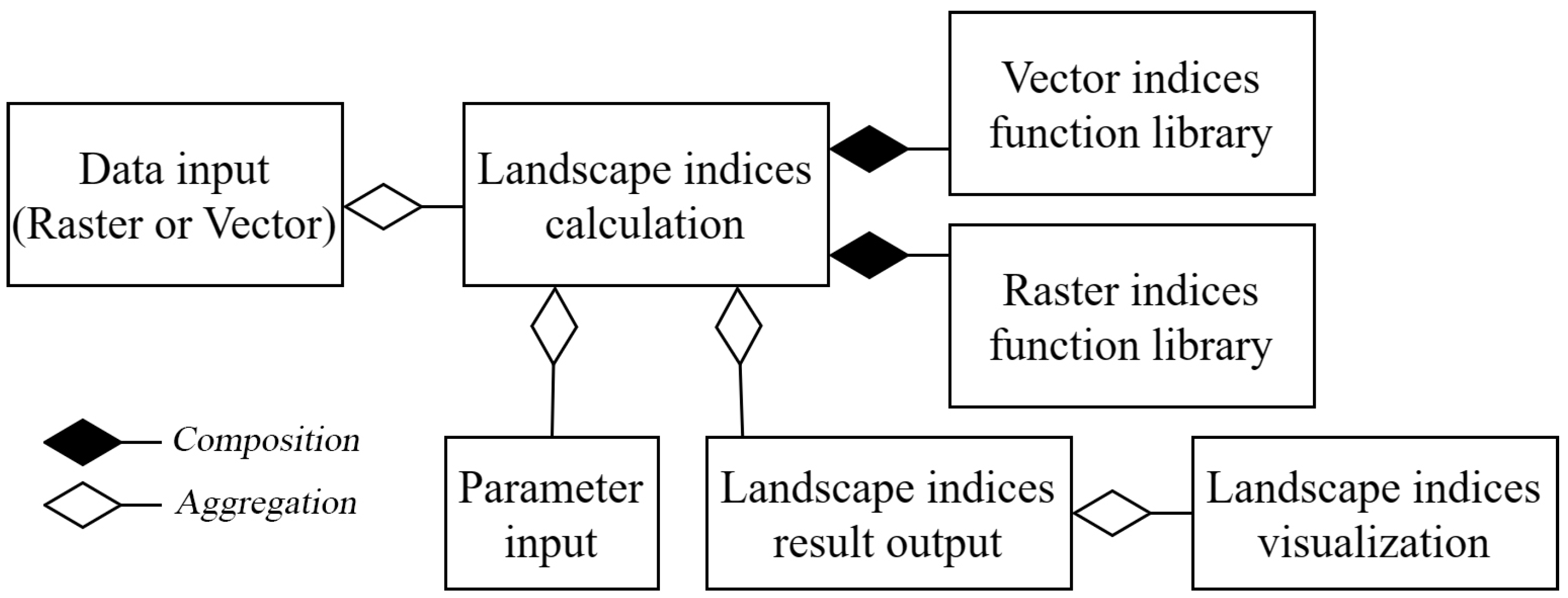
To achieve the goal, Vector and Raster Landscape Indices (VARLI) software (Developers: Yaqi Huang; Software available: https://drive.google.com/file/d/1v0DPBofGeV0tGDy61zI8E_G0Lo_TaBHm/view?usp=sharing (accessed on 3 July 2024); Programming language: Python 39; Integrated development environment: PyCharm; Program size: 200 MB) was designed through secondary development in QGIS. The class diagram of VARLI is shown in the Figure 1; it is structured around the core class “Landscape_indices_calculation”. It is based on the data obtained from the “Data_input” class and the parameters input by the user through the “Parameter_input” class. The program then invokes the calculation functions corresponding to the indices from the “Vector_indices_function_library” class and “Raster_indices_function_library” class. Finally, it can output the calculated indices results and visualize them spatially.
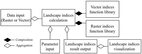
Figure 1.
Class diagram of the VARLI. Black diamond (composition) represents the relationship between the whole and its parts, where the parts cannot exist independently of the whole; the black diamond points to the whole. White diamond (aggregation) represents the relationship between the whole and its parts, where the parts can exist independently of the whole; the white diamond points to the whole.
2.2. Raster–Vector Integration Framework
Spatial data are commonly categorized into two main structures: vector data and raster data. Vector data utilize points, lines, polygons, and their combinations from Euclidean geometry to represent geographical entities. This form of data organization enables precise definition of location, length, area, and other attributes of geographical entities. It is characterized by the implicit representation of attributes and clear delineation of positions. On the other hand, raster data organize the landscape into regular grids, with each grid cell assigned at least one corresponding attribute value to represent geographical entities. Each grid cell corresponds to one attribute in a band, representing a discrete numerical value in space. Raster data are characterized by the implicit representation of positions and clear delineation of attributes.
In PMM, landscape indices calculated from vector data tend to be more precise; however, the data structure is more complex, so computers require more time to process it. Conversely, landscape indices derived from raster data demonstrate scale effects, wherein the sizes of raster cells impact the resulting indices. Nonetheless, raster data structures are comparatively simpler, resulting in quicker computations under lower raster resolutions. For high-precision requirements, it is recommended to compute landscape indices using vector data. Conversely, when approximate results suffice, raster data can be employed. Consider two scenarios: if a user possesses vector data and requires precise results, direct computation of landscape indices in vector format is recommended. However, for expedient decision-making, converting vector data into raster format by adjusting raster cell sizes is advantageous. In another scenario, if the user has high-resolution raster data with slow processing speeds, converting them to vector format is a viable option. Nevertheless, at lower data resolutions, converting raster data to vector may introduce transformation errors, suggesting that using raster data for computing landscape indices remains a preferable choice.
Fragstats [34] encompasses a comprehensive range of landscape indices, several of which are widely utilized by scholars. Consulting the landscape indices provided in Fragstats, the landscape indices’ summary provided by this tool is outlined in Table 2, featuring acronyms for each index. Detailed descriptions of these indices can be found in Appendix A and Appendix B. At the vector data level, 165 landscape indices are calculated, covering dimensions such as area–edge, core area, contrast, shape, aggregation, and diversity across patch, class, and landscape scales (as indicated in the green and blue sections of Table 2). For raster data, approximately 238 landscape indices are computed across the same dimensions and scales (as depicted in the green, blue, and orange sections of Table 2). Certain landscape indices require adjustments based on data type. For instance, indices such as SHAPE, FRAC, and LSI, highlighted in the blue section of Table 2, require correction for perimeter–area ratio discrepancies. For raster data, a square standard with a correction parameter of 0.25 is adopted to rectify size discrepancies in perimeter–area ratios. Conversely, for vector data, a circular standard is employed for this purpose. Formulas and explanations for these calculations are provided in Appendix B.
Table 2.
Summary table of landscape indices. (The expanded form of these indices can be found in Appendix A and Appendix B [34]), Green cells indicate landscape indices calculated at both the vector and raster data levels, orange cells indicate landscape indices calculated at the raster data level, and blue cells indicate that the calculation method of this landscape indices differs between the vector and raster data levels. And statistics include six statistical indicators: MN, AM, MD, RA, SD, and CV.
The integrated vector–raster framework devised is depicted in Figure 2. Users have the flexibility to input either vector or raster data for landscape indices’ calculation. Before computing the landscape indices, the tool conducts an additional check: is there a need to convert the data format? Subsequently, the tool employs functions corresponding to the data type in the landscape-index calculation function library to compute the landscape indices and obtain the calculation results. For vector data, landscape indices are computed by invoking the API for geometric features of vector elements. The code for each index is delineated within the Vector_indices_function_library depicted in Figure 1. Conversely, raster data require the use of matrix operations to calculate landscape indices. The code for each index within this context is encapsulated within the Raster_indices_function_library, as illustrated in Figure 1. By employing different methods for calculating landscape indices for vector and raster data, not only can the problem of data loss during vector–raster conversion be avoided, thereby reducing errors in landscape quantification, but it also provides a choice: for large datasets of vector data, converting them into raster format for calculation is a viable option. This is particularly advantageous when the raster-cell size is significantly smaller than the overall landscape extent, making the disparities between landscape indices computed from vector and raster data negligible. Hence, opting for the computationally efficient raster data format for calculating landscape indices emerges as the preferred choice. Moreover, when computing edge-related landscape indices for raster data, converting them into vector format can effectively address concerns regarding biased edge values.
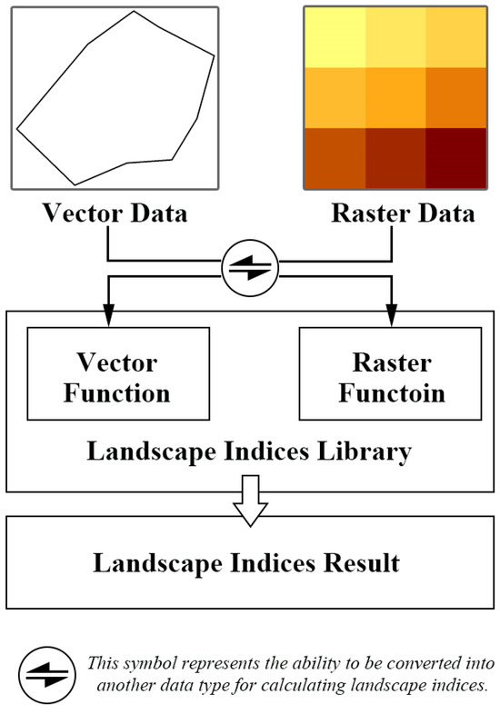
Figure 2.
Integrated vector–raster landscape-index calculation method.
2.3. Landscape-Index Visualization
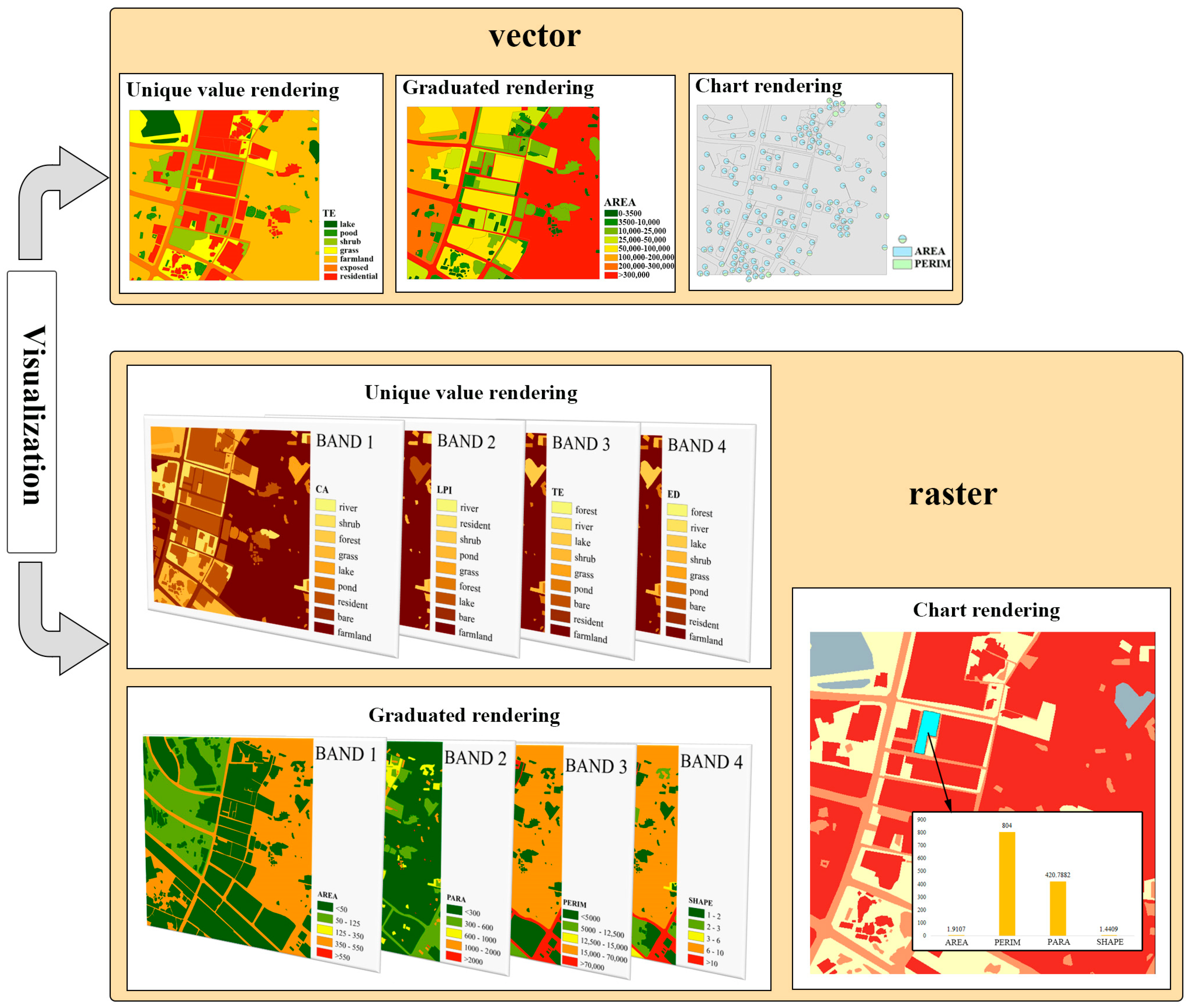
Visualizing the results of landscape indices’ calculations plays a crucial role in enhancing the comprehension of spatial information within geographic landscape patterns. This visualization enables the observation of spatial distribution and patterns in the data, facilitating decision-makers in quickly grasping the situation and making more informed decisions. In VARLI, the calculation results of landscape indices for vector data can be added to its attribute table, enabling feature-based visualization. Additionally, for raster data, the calculation results of landscape indices are stored as bands, allowing for spatial visualization of the indices in the form of a raster matrix. The visualization methods (Figure 3) primarily consist of three types: unique value rendering, graduated rendering, and chart rendering.
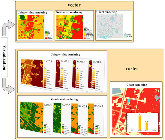
Figure 3.
Visualization methods.
2.3.1. Unique Value Rendering
The unique value-rendering method displays data by assigning unique symbols, colors, and styles to different categories. This method is commonly used for discrete data. Class-level landscape indices typically represent statistical information about patches of different landscape categories. Specifically, for patches belonging to the same category but different locations, the same class-level landscape indices usually have the same value. Therefore, this rendering method is generally employed to display class-level landscape indices, helping to distinguish and visualize the spatial differences in index calculation results for different landscape categories, which facilitate further analysis.
2.3.2. Graduated Rendering
Graduated rendering is used to classify data into different categories based on the distribution of their attribute values. Common classification methods include equal interval, natural breaks, geometric intervals, and standard deviation. After classification, each category is assigned a distinct symbol or color to clearly display the differences and distribution of the data. This rendering method is typically used for continuous data. Patch- level landscape indices, which are often used to represent the landscape-attribute information of different patches within a landscape, are numerous and constitute continuous data. Therefore, this rendering method is generally utilized to express spatial distribution of patch-level landscape indices. However, when necessary, it can also be used to display the spatial distribution of class-level landscape indices. Different patches have different landscape indices based on their shapes and spatial characteristics, and visualizing the landscape-index calculation results of each patch spatially facilitates further analysis of the spatial distribution characteristics of the landscape pattern in the area.
2.3.3. Chart Rendering
Chart rendering is utilized to present data on a map in the form of charts, including bar charts, line charts, pie charts, scatter plots, etc. This method enables the display of different landscape indices of the same patch at the same level (such as patch scale, class scale, or landscape scale) in the chart, or the depiction of landscape indices of the same patch at different levels. For instance, comparing the patch-level and class-level landscape indices of a patch through chart rendering can intuitively reflect the spatial information in the landscape pattern. This approach facilitates the visualization and analysis of landscape indices’ data, aiding in the interpretation of spatial patterns and relationships within the landscape.
3. Program Description
3.1. Data Input Module
In the interface, buttons were added to enable the loading of vector and raster data. The current version of VARLI allows for loading vector data in SHP format and raster data in GeoTIFF format. In future versions, the supported vector data inputs’ data formats will include shapefile (SHP), Keyhole Markup Language (KML), GeoJSON, and file geodatabase formats stored in databases. For raster data, supported formats such as GeoTIFF, ASCII Grid, and IMG were used. This section implements functionality by designing functions triggered by button clicks. A mapCanvas is provided in the main interface for displaying vector and raster spatial data. Further functionalities will be developed and implemented in subsequent versions of VARLI.
3.2. Landscape Indices’ Calculation Module
During the landscape indices’ calculation process, the method of raster–vector integration is integrated into VARLI. Users need to input the following parameters: (a) the data layers for which landscape indices need to be calculated; (b) determination of whether the data layer to be calculated is vector or raster data; (c) determination of whether the user needs to convert vector data to raster data or raster data to vector data; (d) the parameters required for calculating landscape indices; and (e) when calculating landscape indices at the class scale, selection of the corresponding classification field to determine the landscape type to which each patch belongs. VARLI requires these five parameters for landscape indices’ calculation. This model offers users a choice: they can obtain landscape-index calculation results either in vector data format or raster data format. The calculations for various functions are contained within a calculation class, which contains functions for calculating each landscape indices. Currently, VARLI can provide the calculation of all landscape indices for vector data and calculation of a few landscape indices for raster data. Additional landscape-index calculation functionalities will be gradually improved in subsequent versions of VARLI.
3.3. Landscape Indices’ Visualization Module
In this module, VARLI enables the display of calculation results of patch-scale, class-scale, and landscape-scale landscape indices in tabular form. Additionally, it offers functionality for exporting data to Excel. After obtaining the calculation results, users can select from various visualization methods to render the indices’ results visually within VARLI. Currently, VARLI offers three rendering methods: single-symbol rendering, unique-value rendering, and graduated rendering. More diverse visualization methods will be provided in future versions for enhanced functionality.
4. Case Study
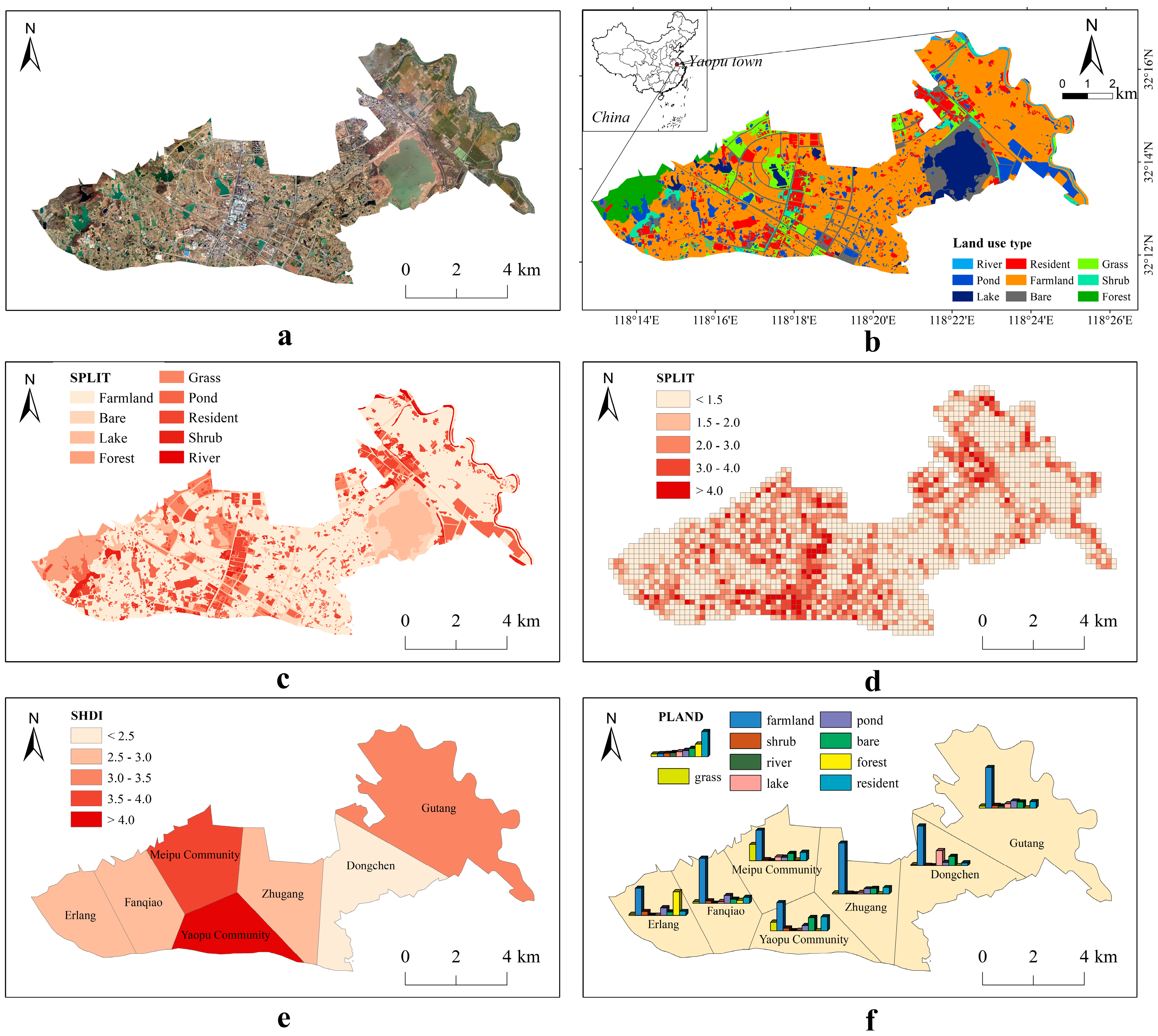
Based on 2020 Google Earth remote-sensing data, this study selected Yaopu Town in Chuzhou City, Anhui Province, China, as a case study. The purpose of this part is to explain the effectiveness of the VARLI. Through visually interpreting and vectorizing the remote-sensing data of Yaopu, obtain the land use data for it in 2020 (Figure 4b). Yaopu is predominantly agricultural, with a significant amount of farmland and rich water resources. The land use in Yaopu is diverse and can be categorized into nine types: grassland, farmland, shrubland, rivers, lakes, residential areas, ponds, bare land, and forests.
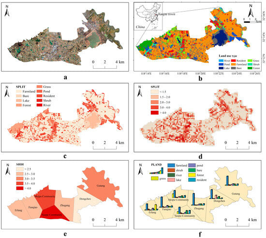
Figure 4.
Spatial distribution visualization results of landscape indices based on land use data for Yaopu Town. (a) Google Earth remote-sensing imagery of Yaopu Town in 2020. (b) Land use data of Yaopu Town in 2020. (c) SPLIT results for different land use types (unique value rendering). (d) Grid-scale SPLIT results (graduated rendering). (e) Regional-scale SHDI results (graduated rendering). (f) Regional-scale PLAND results for different land use types (chart rendering).
The landscape of Yaopu was measured using three indices: SPLIT (splitting index), SHDI (Shannon’s diversity index), and PLAND (percentage of landscape). SPLIT is used to assess the degree of landscape fragmentation; a higher SPLIT value indicates more severe fragmentation of patches within the landscape, while a lower SPLIT value suggests that the patches are more aggregated and continuous. SHDI measures the quantity and distribution of different landscape types, reflecting the landscape’s heterogeneity. PLAND indicates the dominant land use type within the landscape.
The visualization of SPLIT indices for different land use types is rendered using unique values (Figure 4c). This allows for a direct observation of the fragmentation levels of different land use types. To capture local phenomena effectively, a grid with 200 m sides was created to cover the study area. The SPLIT index measured fragmentation within each grid cell and was visualized using graduated rendering (Figure 4d). Consistent with Figure 4c, the central and western regions of the study area exhibit higher landscape fragmentation. Based on the locations of the seven communities and villages within the study area, the area was divided into different administrative regions using Thiessen polygons. Then, the SHDI indices for these regions were calculated and visualized using graduated rendering (Figure 4e). The results suggest that the SHDI values for Yaopu Community and Meipu Community are relatively higher compared to the results of other regions. This indicates a greater diversity and more even distribution of landscape types, which may imply higher landscape heterogeneity in these communities. Additionally, the PLAND metric was used to measure the proportion of different land use types across various regions (Figure 4f). It can be observed that farmland predominates the overall study area, with higher forest cover in the western area. Grassland is more prevalent in Meipu Community and Yaopu Community compared to other areas, and Dongchen has a significant proportion of lake coverage.
The choice of visualization-rendering methods may vary depending on different objectives. But the method of spatial visualization for landscape indices demonstrates the spatial distribution of landscape indices. Since the results are written into the attribute tables of vector features and the bands of raster features, this provides a foundation for further spatial analysis, such as Moran’s I index analysis and geographically weighted regression.
5. Discussion
This paper proposes a framework for calculating landscape indices by integrating vector and raster data. It includes methods for visualizing these landscape indices. Using Yaopu Town as a case study, the spatial distribution of landscape indices is analyzed from the perspectives of landscape type, grid, and region. It demonstrates that visualizing landscape indices is beneficial for analyzing their spatial distribution characteristics.
This paper calculates landscape indices in different dimensions by referencing the formulas provided by Fragstats. Some formulas of landscape indices based on vector data are adjusted according to vector standards in VARLI. Currently, VARLI offers a rich array of landscape indices for vector data, and it will continue to expand the landscape indices of raster data in future work.
Based on the vector data of Yaopu Town, the data were converted into raster data with a 1 m pixel size. Then, the landscape-index results were obtained using VARLI, VecLI, and Fragstats software, respectively. The calculation results from VARLI were compared with those from VecLI and Fragstats, using three statistical measures: Standard Deviation of Absolute Error, Pearson Correlation, and t-test (Table 3). VecLI and Fragstats provide a comprehensive range of landscape indices for both vector and raster data. Comparing VARLI’s landscape indices with those from VecLI and Fragstats can verify the accuracy of VARLI’s results.
Table 3.
Comparison of landscape-index results between VARLI, VECLI, and Fragstats.
From Table 3, it is clear that VARLI exhibits a higher correlation and shows no statistically significant differences compared to VecLI and Fragstats in terms of indices related to the area dimension. In the edge dimension indices, VARLI shows a higher correlation with VecLI and Fragstats, and some indices display significant differences. This may be attributed to VARLI’s method of calculating landscape edges, where it counts the boundary lines between adjacent patches only once. For the shape-dimension indices, it can be observed that there is a high correlation, yet significant differences exist. These differences can be attributed to the variations in the parameters used within the equations (Appendix B). The core area and contrast-dimension indices demonstrate a high correlation with those obtained from Fragstats. The phenomenon of significant differences in some indices could be attributed to the disparities between vector and raster data. Regarding the aggregation and diversity dimensions, it is clear that the results of VARLI are consistent with Fragstats, and it can demonstrate VARLI’s accuracy.
In general, VARLI offers the following advantages:
- It provides rich landscape indices based on vector data and some indices based on raster data, addressing the limitation of existing software that only calculates landscape indices for a single data type.
- It includes three visualization methods for displaying landscape metric results.
- It is open-access and designed for ease of use.
On the other hand, VARLI has some limitations:
- It exhibits lower computational efficiency when processing large volumes of land use data. Thus, the algorithm still needs further optimization in the future.
- Currently, there are limitations for VARLI in displaying the landscape indices derived from raster data, primarily including those reported by Fragstats. In subsequent work, it would be beneficial to focus on incorporating additional indices that are useful for ecological assessment into VARLI.
6. Conclusions and Further Work
We propose an integrated framework that generates landscape indices based on vector and raster data. This framework includes functionality for visualizing indices, allowing for the spatial visualization of indices, which facilitates the observation of their spatial distribution and further analysis. A comparison of the landscape indices calculated by VARLI with those obtained from VecLI and Fragstats shows that the results from VARLI are partially consistent with those from other open-source software, while also exhibiting some differences. To advance landscape ecology further, we recommend the implementation of the following functionalities in the future:
- Developing a web-based application or tool for calculating landscape indices: Currently, landscape indices are mostly calculated using locally installed software, which consumes computer memory. Users need to download and install the software when they need to use it. Subsequent work should further explore the possibility of calculating landscape indices on the web and analyzing and computing landscape indices in an online environment. This facilitates the sharing of index calculation methods, allowing for adjustments and improvements based on calculated results and user feedback. More importantly, it can achieve cross-platform compatibility for landscape-index calculations.
- The functionality of performing addition, subtraction, multiplication, and division operations among landscape indices can be enhanced, and if possible, relevant functions could also be introduced. While organizing the formulas for calculating landscape indices, it was discovered that most indices are composed of a few basic elements, such as FRAC and SHAPE, as detailed in Appendix B. Both indices are derived from the perimeter and area of patch, differing only in their respective functions. Since many indices are constructed from these fundamental elements, performing these operations can enhance user understanding of the indices. For instance, the indices PD and AREA_MN are highly correlated, and selecting both could lead to data redundancy. Adding this functionality will make users more considerate when making their selections. What is more, the ability to recombine these basic elements to create new indices could further unlock the potential value of landscape indices.
- Additional geospatial data mining tools can be incorporated. Subsequently, the system can be enhanced by integrating machine-learning algorithms such as logistic regression analysis, principal component analysis, support vector machines, neural networks, and random forest regression. I believe that integrating landscape index calculations with other geospatial data mining tools will provide model support for the in-depth exploration of the information contained within landscape indices and the analysis of landscape patterns.
Author Contributions
Conceptualization, Yaqi Huang, Minrui Zheng and Xinqi Zheng; data curation, Yaqi Huang; formal analysis, Fei Xiao; funding acquisition, Minrui Zheng and Xinqi Zheng; investigation, Xinqi Zheng; methodology, Yaqi Huang, Minrui Zheng, Tianle Li, Fei Xiao and Xinqi Zheng; software, Yaqi Huang and Tianle Li; supervision, Tianle Li; writing—original draft, Yaqi Huang; writing—review and editing, Minrui Zheng, Tianle Li, Fei Xiao and Xinqi Zheng. All authors have read and agreed to the published version of the manuscript.
Funding
This research was funded by the National Natural Science Foundation of China, grant number 42201471; the Beijing Social Science Foundation, grant number 2022YJC264; the Key Program of National Natural Science Foundation of China, grant number 72033005; and the Third Xinjiang Scientific Expedition of the Key Research and Development Program by Ministry of Science and Technology of the People’s Republic of China, grant number 2022xjkk1104.
Data Availability Statement
Data are available upon request to the authors.
Acknowledgments
The authors express gratitude to OpenAI for providing ChatGPT 3.5 to assist in writing the program, enabling the implementation of some functionalities within the program.
Conflicts of Interest
The authors declare no conflicts of interest.
Appendix A
List of full names of landscape indices calculated in the tool. (Referenced from Fragstats, with calculation formulas and detailed explanations provided)
| Metric Number | Level | Acronym | Name |
| 1 | P | AREA | Patch area |
| 2 | P | PERIM | Patch perimeter |
| 3 | P | GYRATE | Radius of gyration |
| 4 | P | PARA | Perimeter–area ratio |
| 5 | P | SHAPE | Shape index |
| 6 | P | FRAC | Fractal dimension index |
| 7 | P | CIRCLE | Related circumscribing circle |
| 8 | P | CONTIG | Contiguity index |
| 9 | P | CORE | Core area |
| 10 | P | NCORE | Number of core areas |
| 11 | P | CAI | Core area index |
| 12 | P | ECON | Edge contrast index |
| 13 | P | ENN | Euclidean nearest-neighbor distance |
| 14 | P | PROX | Proximity index |
| 15 | P | SIMI | Similarity index |
| 16 | C | CA/TA | Total area (class) |
| 17 | C | PLAND | Percentage of landscape |
| 18 | C | CPLAND | Core area percentage of landscape |
| 19 | C | CLUMPY | Clumpiness index |
| 20 | C | NLSI | Normalized landscape shape index |
| 21 | L | CA/TA | Total area (landscape) |
| 22 | L | CONTAG | Contagion |
| 23 | L | PR | Patch richness |
| 24 | L | PRD | Patch richness density |
| 25 | L | RPR | Relative patch richness |
| 26 | L | SHDI | Shannon’s diversity index |
| 27 | L | SIDI | Simpson’s diversity index |
| 28 | L | MSIDI | Modified Simpson’s diversity index |
| 29 | L | SHEI | Shannon’s evenness index |
| 30 | L | SIEI | Simpson’s evenness index |
| 31 | L | MSIEI | Modified Simpson’s evenness index |
| 32 | C,L | LPI | Largest patch index |
| 33 | C,L | TE | Total edge |
| 34 | C,L | ED | Edge density |
| 35 | C,L | PAFRAC | Perimeter–area fractal dimension |
| 36 | C,L | TCA | Total core area |
| 37 | C,L | NDCA | Number of disjunct core areas |
| 38 | C,L | DCAD | Disjunct core area density |
| 39 | C,L | CWED | Contrast-weighted edge density |
| 40 | C,L | TECI | Total edge contrast index |
| 41 | C,L | CONNECT | Connectance index |
| 42 | C,L | NP | Number of patches |
| 43 | C,L | PD | Patch density |
| 44 | C,L | DIVISION | Landscape division index |
| 45 | C,L | SPLIT | Splitting index |
| 46 | C,L | MESH | Effective mesh size |
| 47 | C,L | IJI | Interspersion juxtaposition index |
| 48 | C,L | PLADJ | Proportion of like adjacencies |
| 49 | C,L | AI | Aggregation index |
| 50 | C,L | LSI | Landscape shape index |
| 51 | C,L | COHESION | Patch cohesion index |
| 52 | C,L | AREA_MN | The mean of patch area |
| 53 | C,L | AREA_AM | The area-weighted mean of patch area |
| 54 | C,L | AREA_MD | The median of patch area |
| 55 | C,L | AREA_RA | The range of variation in patch area |
| 56 | C,L | AREA_SD | The standard deviation of patch area |
| 57 | C,L | AREA_CV | The coefficient of variance of patch area |
| 58 | C,L | GYRATE_MN | The mean of radius of gyration |
| 59 | C,L | GYRATE_AM | The area-weighted mean of radius of gyration |
| 60 | C,L | GYRATE_MD | The median of radius of gyration |
| 61 | C,L | GYRATE_RA | The range of variation in radius of gyration |
| 62 | C,L | GYRATE_SD | The standard deviation of radius of gyration |
| 63 | C,L | GYRATE_CV | The coefficient of variance of radius of gyration |
| 64 | C,L | SHAPE_MN | The mean of shape index |
| 65 | C,L | SHAPE_AM | The area-weighted mean of shape index |
| 66 | C,L | SHAPE_MD | The median of shape index |
| 67 | C,L | SHAPE_RA | The range of variation in shape index |
| 68 | C,L | SHAPE_SD | The standard deviation of shape index |
| 69 | C,L | SHAPE_CV | The coefficient of variance of shape index |
| 70 | C,L | FRAC_MN | The mean of fractal dimension index |
| 71 | C,L | FRAC_AM | The area-weighted mean of fractal dimension index |
| 72 | C,L | FRAC_MD | The median of fractal dimension index |
| 73 | C,L | FRAC_RA | The range of variation in fractal dimension index |
| 74 | C,L | FRAC_SD | The standard deviation of fractal dimension index |
| 75 | C,L | FRAC_CV | The coefficient of variance of fractal dimension index |
| 76 | C,L | PARA_MN | The mean of perimeter–area ratio |
| 77 | C,L | PARA_AM | The area-weighted mean of perimeter–area ratio |
| 78 | C,L | PARA_MD | The median of perimeter–area ratio |
| 79 | C,L | PARA_RA | The range of variation in perimeter–area ratio |
| 80 | C,L | PARA_SD | The standard deviation of perimeter–area ratio |
| 81 | C,L | PARA_CV | The coefficient of variance in perimeter–area ratio |
| 82 | C,L | CIRCLE_MN | The mean of related circumscribing circle |
| 83 | C,L | CIRCLE_AM | The area-weighted mean of related circumscribing circle |
| 84 | C,L | CIRCLE_MD | The median of related circumscribing circle |
| 85 | C,L | CIRCLE_RA | The range of variation in related circumscribing circle |
| 86 | C,L | CIRCLE_SD | The standard deviation of related circumscribing circle |
| 87 | C,L | CIRCLE_CV | The coefficient of variance of related circumscribing circle |
| 88 | C,L | CONTIG_MN | The mean of contiguity index |
| 89 | C,L | CONTIG_AM | The area-weighted mean of contiguity index |
| 90 | C,L | CONTIG_MD | The median of contiguity index |
| 91 | C,L | CONTIG_RA | The range of variation in contiguity index |
| 92 | C,L | CONTIG_SD | The standard deviation of contiguity index |
| 93 | C,L | CONTIG_CV | The coefficient of variance of contiguity index |
| 94 | C,L | CORE_MN | The mean of core area |
| 95 | C,L | CORE_AM | The area-weighted mean of core area |
| 96 | C,L | CORE_MD | The median of core area |
| 97 | C,L | CORE_RA | The range of variation in core area |
| 98 | C,L | CORE_SD | The standard deviation of core area |
| 99 | C,L | CORE_CV | The coefficient of variance of core area |
| 100 | C,L | DCORE_MN | The mean of disjunct core area |
| 101 | C,L | DCORE_AM | The area-weighted mean of disjunct core area |
| 102 | C,L | DCORE_MD | The median of disjunct core area |
| 103 | C,L | DCORE_RA | The range of variation in disjunct core area |
| 104 | C,L | DCORE_SD | The standard deviation of disjunct core area |
| 105 | C,L | DCORE_CV | The coefficient of variance of disjunct core area |
| 106 | C,L | CAI_MN | The mean of core area index |
| 107 | C,L | CAI_AM | The area-weighted mean of core area index |
| 108 | C,L | CAI_MD | The median of core area index |
| 109 | C,L | CAI_RA | The range of variation in core area index |
| 110 | C,L | CAI_SD | The standard deviation of core area index |
| 111 | C,L | CAI_CV | The coefficient of variance of core area index |
| 112 | C,L | PROX_MN | The mean of proximity index |
| 113 | C,L | PROX_AM | The area-weighted mean of proximity index |
| 114 | C,L | PROX_MD | The median of proximity index |
| 115 | C,L | PROX_RA | The range of variation in proximity index |
| 116 | C,L | PROX_SD | The standard deviation of proximity index |
| 117 | C,L | PROX_CV | The coefficient of variance of proximity index |
| 118 | C,L | SIMI_MN | The mean of similarity index |
| 119 | C,L | SIMI_AM | The area-weighted mean of similarity index |
| 120 | C,L | SIMI_MD | The median of similarity index |
| 121 | C,L | SIMI_RA | The range of variation in similarity index |
| 122 | C,L | SIMI_SD | The standard deviation of similarity index |
| 123 | C,L | SIMI_CV | The coefficient of variance of similarity index |
| 124 | C,L | ENN_MN | The mean of Euclidean nearest-neighbor distance |
| 125 | C,L | ENN_AM | The area-weighted mean of Euclidean nearest-neighbor distance |
| 126 | C,L | ENN_MD | The median of Euclidean nearest-neighbor distance |
| 127 | C,L | ENN_RA | The range of variation in Euclidean nearest-neighbor distance |
| 128 | C,L | ENN_SD | The standard deviation of Euclidean nearest-neighbor distance |
| 129 | C,L | ENN_CV | The coefficient of variance of Euclidean nearest-neighbor distance |
| 130 | C,L | ECON_MN | The mean of edge contrast index |
| 131 | C,L | ECON_AM | The area-weighted mean of edge contrast index |
| 132 | C,L | ECON_MD | The median of edge contrast index |
| 133 | C,L | ECON_RA | The range of variation in edge contrast index |
| 134 | C,L | ECON_SD | The standard deviation of edge contrast index |
| 135 | C,L | ECON_CV | The coefficient of variance of edge contrast index |
Appendix B
The description of special landscape indices.
| Name (Abbreviation) | Formula | Parameters |
| Patch shape (SHAPE) | : perimeter (m) of patch ij. : area (m2) of patch ij. | |
| Unit | Range | Description |
| / | ≥1 | Shape index of the patch: When the patch is circular, SHAPE = 1; as the patch shape becomes more complex, SHAPE increases gradually. |
| Name (Abbreviation) | Formula | Parameters |
| Fractal dimension (FRAC) | : perimeter (m) of patch ij. : area (m2) of patch ij. | |
| Unit | Range | Description |
| / | [1,2] | Fractal dimension of the patch: When the patch is circular, FRAC = 1; as the patch shape becomes more complex, FRAC approaches 2. |
| Name (Abbreviation) | Formula | Parameters |
| Landscape-shape index in class level (LSI) (class) | : total length (m) of edge in landscape between patch types (classes) i and k. : total landscape area (m2). | |
| Unit | Range | Description |
| / | ≥1 | When the patch type i consists of a single square, LSI = 1; LSI increases as the shapes of patches within the patch type become more irregular. |
| Name (Abbreviation) | Formula | Parameters |
| Landscape-shape index in landscape level (LSI) (landscape) | : the total length (m) of edges within the landscape, including boundary edges. : total area (m2) of the landscape. | |
| Unit | Range | Description |
| / | ≥1 | The landscape-shape index of patches in the landscape. When the landscape consists of a single square, LSI = 1; LSI increases as the shape of patches in the landscape becomes more irregular or as the total edge length within the landscape increases. |
References
- Forman, R.T.T.; Godron, M. Landscape Ecology; Wiley: New York, NY, USA, 1986. [Google Scholar]
- Jianguo, W. Landscape ecology-concepts and theories. Chin. J. Ecol. 2000, 19, 42–52. [Google Scholar]
- Ryu, S.R.; Chen, J.; Zheng, D.; Lacroix, J.J. Relating surface fire spread to landscape structure: An application of FARSITE in a managed forest landscape. Landsc. Urban Plan. 2007, 83, 275–283. [Google Scholar] [CrossRef]
- Thiele, J.; Kellner, S.; Buchholz, S.; Schirmel, J. Connectivity or area: What drives plant species richness in habitat corridors? Landsc. Ecol. 2018, 33, 173–181. [Google Scholar] [CrossRef]
- Zhang, R.; Li, S.; Wei, B.; Zhou, X. Characterizing production–living–ecological space evolution and its driving factors: A case study of the chaohu lake basin in China from 2000 to 2020. ISPRS Int. J. Geo-Inf. 2022, 11, 447. [Google Scholar]
- Hou, B.; Wei, C.; Liu, X.; Meng, Y.; Li, X. Assessing Forest Landscape Stability through Automatic Identification of Landscape Pattern Evolution in Shanxi Province of China. Remote Sens. 2023, 15, 545. [Google Scholar] [CrossRef]
- Forman, R.T.T.; Godron, M. Patches and structural components for a landscape ecology. BioScience 1981, 31, 733–740. [Google Scholar]
- McGarigal, K.; Cushman, S.A. The Gradient Concept of Landscape Structure. In Issues and Perspectives in Landscape Ecology; Cambridge University Press: Cambridge, UK, 2005; pp. 112–119. [Google Scholar]
- Bolliger, J.; Wagner, H.H.; Turner, M.G. Identifying and quantifying landscape patterns in space and time. In A Changing World: Challenges for Landscape Research; Springer: Dordrecht, The Netherlands, 2007; pp. 177–194. [Google Scholar]
- Lausch, A.; Blaschke, T.; Haase, D.; Herzog, F.; Syrbe, R.U.; Tischendorf, L.; Walz, U. Understanding and quantifying landscape structure—A review on relevant process characteristics, data models and landscape metrics. Ecol. Modell. 2015, 295, 31–41. [Google Scholar] [CrossRef]
- Nowosad, J.; Stepinski, T.F. Information theory as a consistent framework for quantification and classification of landscape patterns. Landsc. Ecol. 2019, 34, 2091–2101. [Google Scholar] [CrossRef]
- Huang, C.; Yang, J.; Jiang, P. Assessing impacts of urban form on landscape structure of urban green spaces in China using Landsat images based on Google Earth Engine. Remote Sens. 2018, 10, 1569. [Google Scholar] [CrossRef]
- Shannon, C.E. A mathematical theory of communication. Bell Syst. Tech. J. 1948, 27, 379–423. [Google Scholar] [CrossRef]
- Simpson, E.H. Measurement of diversity. Nature 1949, 163, 688. [Google Scholar] [CrossRef]
- Tsallis, C. Entropic nonextensivity: A possible measure of complexity. Chaos Solitons Fractals 2002, 13, 371–391. [Google Scholar] [CrossRef]
- Cushman, S.A. Entropy in landscape ecology: A quantitative textual multivariate review. Entropy 2021, 23, 1425. [Google Scholar] [CrossRef] [PubMed]
- Burrough, P.A. Fractal dimensions of landscapes and other environmental data. Nature 1981, 294, 240–242. [Google Scholar] [CrossRef]
- Alados, C.L.; Pueyo, Y.; Giner, M.L.; Navarro, T.; Escos, J.; Barroso, F.; Cabezudo, B.; Emlen, J.M. Quantitative characterization of the regressive ecological succession by fractal analysis of plant spatial patterns. Ecol. Modell. 2003, 163, 1–17. [Google Scholar] [CrossRef]
- Saura, S.; Estreguil, C.; Mouton, C.; Rodríguez-Freire, M. Network analysis to assess landscape connectivity trends: Application to European forests (1990–2000). Ecol. Indic. 2011, 11, 407–416. [Google Scholar] [CrossRef]
- Foltête, J.C.; Clauzel, C.; Vuidel, G. A software tool dedicated to the modelling of landscape networks. Environ. Modell. Softw. 2012, 38, 316–327. [Google Scholar] [CrossRef]
- de la Barra, F.; Alignier, A.; Reyes-Paecke, S.; Duane, A.; Miranda, M.D. Selecting graph metrics with ecological significance for deepening landscape characterization: Review and applications. Land 2022, 11, 338. [Google Scholar] [CrossRef]
- Merrick, M.J.; Koprowski, J.L. Circuit theory to estimate natal dispersal routes and functional landscape connectivity for an endangered small mammal. Landsc. Ecol. 2017, 32, 1163–1179. [Google Scholar] [CrossRef]
- Liu, X.; Liu, D.; Zhao, H.; He, J.; Liu, Y. Exploring the spatio-temporal impacts of farmland reforestation on ecological connectivity using circuit theory: A case study in the agro-pastoral ecotone of North China. J. Geog. Sci. 2020, 30, 1419–1435. [Google Scholar] [CrossRef]
- Landau, V.A.; Shah, V.B.; Anantharaman, R.; Hall, K.R. Omniscape. jl: Software to compute omnidirectional landscape connectivity. J. Open Source Softw. 2021, 6, 2829. [Google Scholar] [CrossRef]
- Cushman, S.A.; McGarigal, K.; Neel, M.C. Parsimony in landscape metrics: Strength, universality, and consistency. Ecol. Indic. 2008, 8, 691–703. [Google Scholar] [CrossRef]
- Kienast, F.; Frick, J.; van Strien, M.J.; Hunziker, M. The Swiss Landscape Monitoring Program—A comprehensive indicator set to measure landscape change. Ecol. Modell. 2015, 295, 136–150. [Google Scholar] [CrossRef]
- Dong, J.; Dai, W.; Shao, G.; Xu, J. Ecological network construction based on minimum cumulative resistance for the city of Nanjing, China. ISPRS Int. J. Geo-Inf. 2015, 4, 2045–2060. [Google Scholar]
- Li, M.; Luo, G.; Li, Y.; Qin, Y.; Huang, J.; Liao, J. Effects of landscape patterns and their changes on ecosystem health under different topographic gradients: A case study of the Miaoling Mountains in southern China. Ecol. Indic. 2023, 154, 110796. [Google Scholar] [CrossRef]
- Xiao, C.; Wang, Y.; Yan, M.; Chiaka, J.C. Impact of cross-border transportation corridors on changes of land use and landscape pattern: A case study of the China-Laos railway. Landsc. Urban Plan. 2024, 241, 104924. [Google Scholar] [CrossRef]
- Adler, K.; Jedicke, E. Landscape metrics as indicators of avian community structures—A state of the art review. Ecol. Indic. 2022, 145, 109575. [Google Scholar] [CrossRef]
- Frazier, A.E.; Kedron, P. Comparing forest fragmentation in Eastern US forests using patch-mosaic and gradient surface models. Ecol. Inform. 2017, 41, 108–115. [Google Scholar] [CrossRef]
- Chang, S.; Jiang, Q.; Wang, Z.; Xu, S.; Jia, M. Extraction and spatial–temporal evolution of urban fringes: A case study of changchun in Jilin Province, China. ISPRS Int. J. Geo-Inf. 2018, 7, 241. [Google Scholar]
- Xu, M.; Niu, L.; Wang, X.; Zhang, Z. Evolution of farmland landscape fragmentation and its driving factors in the Beijing-Tianjin-Hebei region. J. Clean. Prod. 2023, 418, 138031. [Google Scholar] [CrossRef]
- McGarigal, K.; Marks, B.J. FRAGSTATS: Spatial Pattern Analysis Program for Quantifying Landscape Structure; Gen. Tech. Rep. PNW-GTR-351; U.S. Department of Agriculture, Forest Service, Pacific Northwest Research Station: Portland, OR, USA, 1995.
- Yao, Y.; Cheng, T.; Sun, Z.; Li, L.; Chen, D.; Chen, Z.; Wei, J.; Guan, Q. VecLI: A framework for calculating vector landscape indices considering landscape fragmentation. Environ. Modell. Softw. 2022, 149, 105325. [Google Scholar] [CrossRef]
- Bettinger, P.; Bradshaw, G.A.; Weaver, G.W. Effects of geographic information system vector–raster–vector data conversion on landscape indices. Can. J. For. Res. 1996, 26, 1416–1425. [Google Scholar] [CrossRef]
- Wade, T.G.; Wickham, J.D.; Nash, M.S.; Neale, A.C.; Riitters, K.H.; Jones, K.B. A comparison of vector and raster GIS methods for calculating landscape metrics used in environmental assessments. Photogramm. Eng. Remote Sens. 2003, 69, 1399–1405. [Google Scholar] [CrossRef]
- Saura, S.; Torné, J. Conefor Sensinode 2.2: A software package for quantifying the importance of habitat patches for landscape connectivity. Environ. Modell. Softw. 2009, 24, 135–139. [Google Scholar]
- Baker, W.L.; Cai, Y. The r.le programs for multiscale analysis of landscape structure using the GRASS geographical information system. Landsc. Ecol. 1992, 7, 291–302. [Google Scholar] [CrossRef]
- Rempel, R.S.; Kaukinen, D.; Carr, A.P. Patch Analyst and Patch Grid. Ontario Ministry of Natural Resources; Centre for Northern Forest Ecosystem Research: Thunder Bay, ON, Canada, 2012. [Google Scholar]
- Lang, S.; Tiede, D. vLATE Extension für ArcGIS–Vektorbasiertes Tool zur Quantitativen Landschaftsstrukturanalyse. 2003. Available online: https://uni-salzburg.elsevierpure.com/en/publications/vlate-extension-f%C3%BCr-arcgis-vektorbasiertes-tool-zur-quantitativen (accessed on 3 July 2024).
- Yu, M.; Huang, Y.; Cheng, X.; Tian, J. An ArcMap plug-in for calculating landscape metrics of vector data. Ecol. Inform. 2019, 50, 207–219. [Google Scholar] [CrossRef]
- Jung, M. LecoS—A python plugin for automated landscape ecology analysis. Ecol. Inform. 2016, 31, 18–21. [Google Scholar] [CrossRef]
- Zaragozí, B.; Belda, A.; Linares, J.; Martínez-Pérez, J.E.; Navarro, J.T.; Esparza, J. A free and open source programming library for landscape metrics calculations. Environ. Modell. Softw. 2012, 31, 131–140. [Google Scholar] [CrossRef]
- Hesselbarth, M.H.; Sciaini, M.; With, K.A.; Wiegand, K.; Nowosad, J. landscapemetrics: An open-source R tool to calculate landscape metrics. Ecography 2019, 42, 1648–1657. [Google Scholar] [CrossRef]
- QGIS. A Free and Open Source Geographic Information System. 2024. Available online: https://www.qgis.org/ (accessed on 3 July 2024).
- QGIS Development Team. QGIS Geographic Information System. Available online: http://qgis.osgeo.org (accessed on 12 May 2024).
- PyQGIS Developer Cookbook (QGIS 3.34). QGIS Documentation. Available online: https://docs.qgis.org/3.34/en/docs/pyqgis_developer_cookbook/index.html (accessed on 7 March 2024).

Disclaimer/Publisher’s Note: The statements, opinions and data contained in all publications are solely those of the individual author(s) and contributor(s) and not of MDPI and/or the editor(s). MDPI and/or the editor(s) disclaim responsibility for any injury to people or property resulting from any ideas, methods, instructions or products referred to in the content. |
© 2024 by the authors. Licensee MDPI, Basel, Switzerland. This article is an open access article distributed under the terms and conditions of the Creative Commons Attribution (CC BY) license (https://creativecommons.org/licenses/by/4.0/).