
An Integrated Framework for Landscape Indices’ Calculation with Raster–Vector Integration and Its Application Based on QGIS


Abstract
1. Introduction
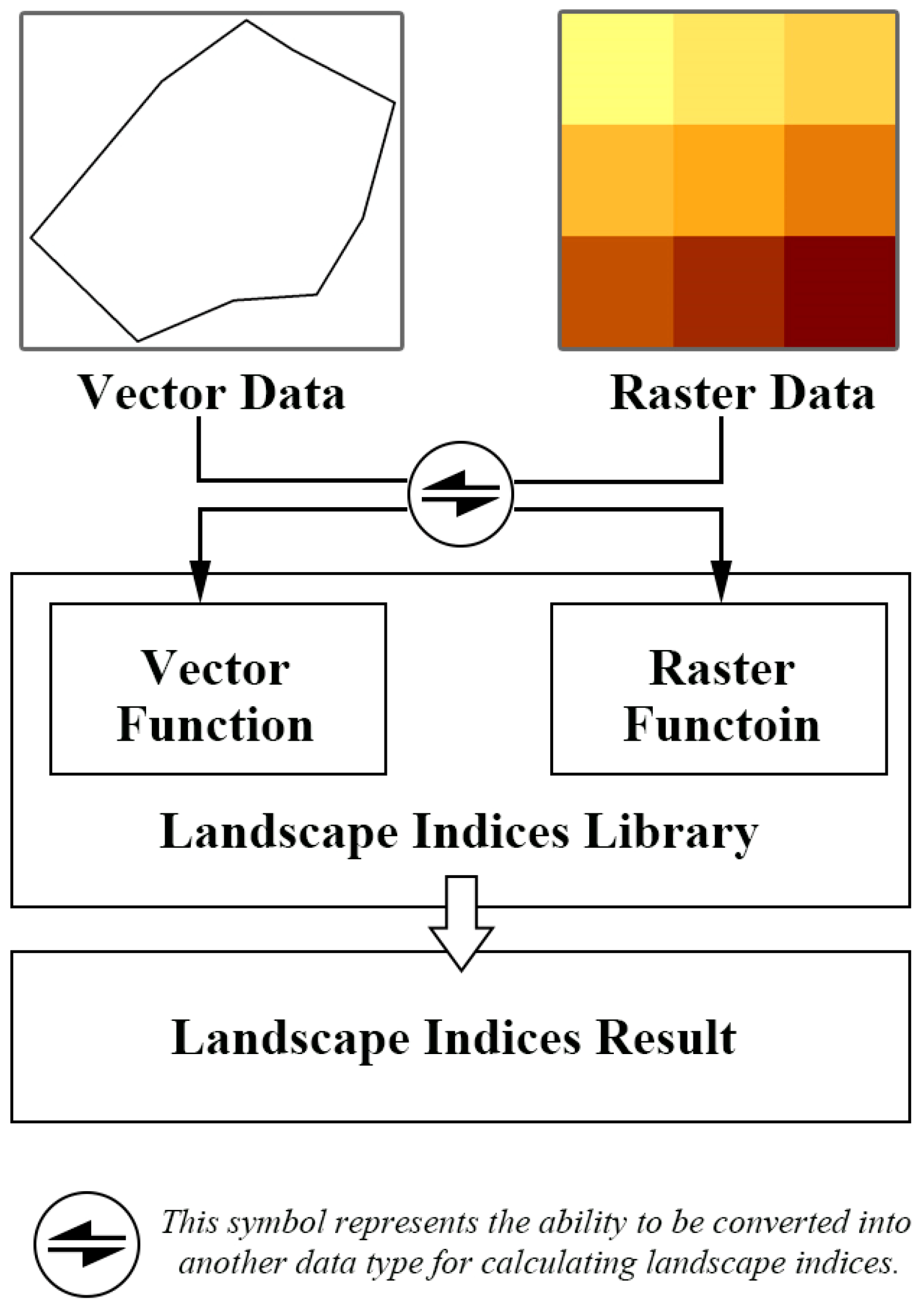
- Based on the Quantum Geographic Information System (QGIS) [46] platform, this study conducted a secondary development to explore methods for integrating vector and raster data for landscape indices. Users can choose to calculate landscape indices using either vector or raster methods according to their needs.
- For vector data, 165 indices are available for selection, while for raster data, 20 indices are available.
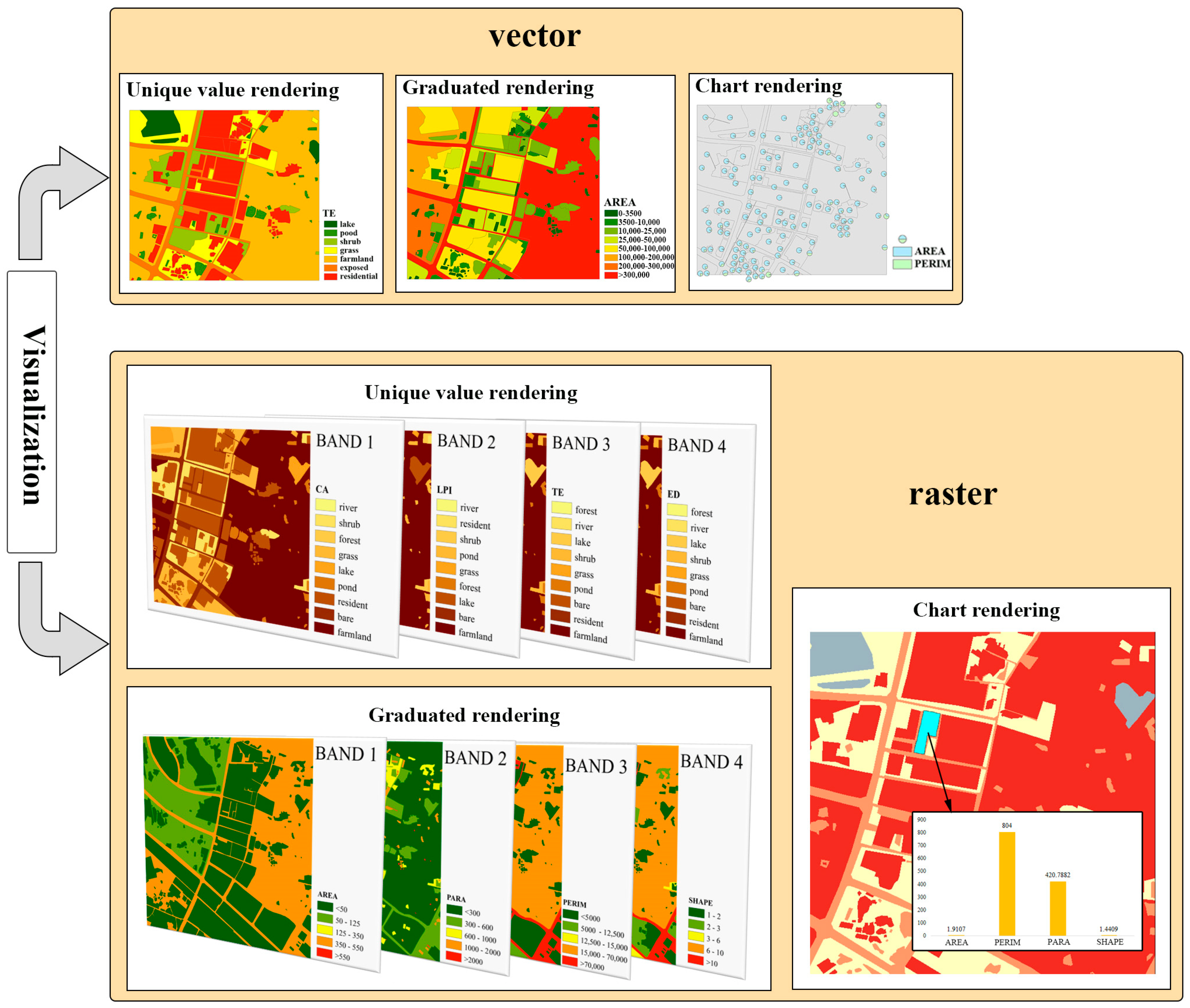
- Three rendering methods are provided for visualizing landscape indices: unique value rendering, graduated rendering, and chart rendering.
2. Methods
2.1. Development Environment and System Architecture
2.2. Raster–Vector Integration Framework
2.3. Landscape-Index Visualization
2.3.1. Unique Value Rendering
2.3.2. Graduated Rendering
2.3.3. Chart Rendering
3. Program Description
3.1. Data Input Module
3.2. Landscape Indices’ Calculation Module
3.3. Landscape Indices’ Visualization Module
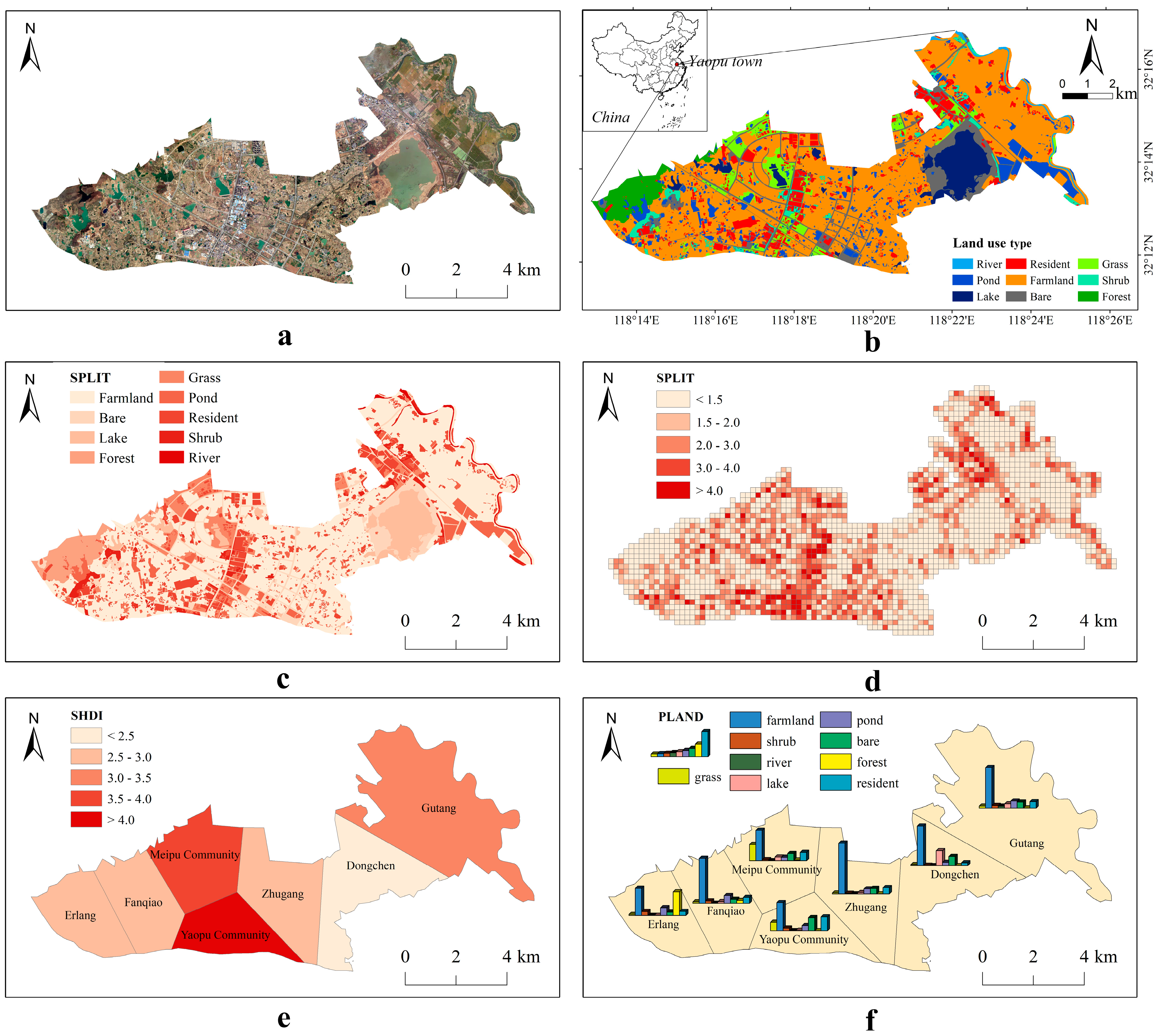
4. Case Study
5. Discussion
- It provides rich landscape indices based on vector data and some indices based on raster data, addressing the limitation of existing software that only calculates landscape indices for a single data type.
- It includes three visualization methods for displaying landscape metric results.
- It is open-access and designed for ease of use.
- It exhibits lower computational efficiency when processing large volumes of land use data. Thus, the algorithm still needs further optimization in the future.
- Currently, there are limitations for VARLI in displaying the landscape indices derived from raster data, primarily including those reported by Fragstats. In subsequent work, it would be beneficial to focus on incorporating additional indices that are useful for ecological assessment into VARLI.
6. Conclusions and Further Work
- Developing a web-based application or tool for calculating landscape indices: Currently, landscape indices are mostly calculated using locally installed software, which consumes computer memory. Users need to download and install the software when they need to use it. Subsequent work should further explore the possibility of calculating landscape indices on the web and analyzing and computing landscape indices in an online environment. This facilitates the sharing of index calculation methods, allowing for adjustments and improvements based on calculated results and user feedback. More importantly, it can achieve cross-platform compatibility for landscape-index calculations.
- The functionality of performing addition, subtraction, multiplication, and division operations among landscape indices can be enhanced, and if possible, relevant functions could also be introduced. While organizing the formulas for calculating landscape indices, it was discovered that most indices are composed of a few basic elements, such as FRAC and SHAPE, as detailed in Appendix B. Both indices are derived from the perimeter and area of patch, differing only in their respective functions. Since many indices are constructed from these fundamental elements, performing these operations can enhance user understanding of the indices. For instance, the indices PD and AREA_MN are highly correlated, and selecting both could lead to data redundancy. Adding this functionality will make users more considerate when making their selections. What is more, the ability to recombine these basic elements to create new indices could further unlock the potential value of landscape indices.
- Additional geospatial data mining tools can be incorporated. Subsequently, the system can be enhanced by integrating machine-learning algorithms such as logistic regression analysis, principal component analysis, support vector machines, neural networks, and random forest regression. I believe that integrating landscape index calculations with other geospatial data mining tools will provide model support for the in-depth exploration of the information contained within landscape indices and the analysis of landscape patterns.
Author Contributions
Funding
Data Availability Statement
Acknowledgments
Conflicts of Interest
Appendix A
| Metric Number | Level | Acronym | Name |
| 1 | P | AREA | Patch area |
| 2 | P | PERIM | Patch perimeter |
| 3 | P | GYRATE | Radius of gyration |
| 4 | P | PARA | Perimeter–area ratio |
| 5 | P | SHAPE | Shape index |
| 6 | P | FRAC | Fractal dimension index |
| 7 | P | CIRCLE | Related circumscribing circle |
| 8 | P | CONTIG | Contiguity index |
| 9 | P | CORE | Core area |
| 10 | P | NCORE | Number of core areas |
| 11 | P | CAI | Core area index |
| 12 | P | ECON | Edge contrast index |
| 13 | P | ENN | Euclidean nearest-neighbor distance |
| 14 | P | PROX | Proximity index |
| 15 | P | SIMI | Similarity index |
| 16 | C | CA/TA | Total area (class) |
| 17 | C | PLAND | Percentage of landscape |
| 18 | C | CPLAND | Core area percentage of landscape |
| 19 | C | CLUMPY | Clumpiness index |
| 20 | C | NLSI | Normalized landscape shape index |
| 21 | L | CA/TA | Total area (landscape) |
| 22 | L | CONTAG | Contagion |
| 23 | L | PR | Patch richness |
| 24 | L | PRD | Patch richness density |
| 25 | L | RPR | Relative patch richness |
| 26 | L | SHDI | Shannon’s diversity index |
| 27 | L | SIDI | Simpson’s diversity index |
| 28 | L | MSIDI | Modified Simpson’s diversity index |
| 29 | L | SHEI | Shannon’s evenness index |
| 30 | L | SIEI | Simpson’s evenness index |
| 31 | L | MSIEI | Modified Simpson’s evenness index |
| 32 | C,L | LPI | Largest patch index |
| 33 | C,L | TE | Total edge |
| 34 | C,L | ED | Edge density |
| 35 | C,L | PAFRAC | Perimeter–area fractal dimension |
| 36 | C,L | TCA | Total core area |
| 37 | C,L | NDCA | Number of disjunct core areas |
| 38 | C,L | DCAD | Disjunct core area density |
| 39 | C,L | CWED | Contrast-weighted edge density |
| 40 | C,L | TECI | Total edge contrast index |
| 41 | C,L | CONNECT | Connectance index |
| 42 | C,L | NP | Number of patches |
| 43 | C,L | PD | Patch density |
| 44 | C,L | DIVISION | Landscape division index |
| 45 | C,L | SPLIT | Splitting index |
| 46 | C,L | MESH | Effective mesh size |
| 47 | C,L | IJI | Interspersion juxtaposition index |
| 48 | C,L | PLADJ | Proportion of like adjacencies |
| 49 | C,L | AI | Aggregation index |
| 50 | C,L | LSI | Landscape shape index |
| 51 | C,L | COHESION | Patch cohesion index |
| 52 | C,L | AREA_MN | The mean of patch area |
| 53 | C,L | AREA_AM | The area-weighted mean of patch area |
| 54 | C,L | AREA_MD | The median of patch area |
| 55 | C,L | AREA_RA | The range of variation in patch area |
| 56 | C,L | AREA_SD | The standard deviation of patch area |
| 57 | C,L | AREA_CV | The coefficient of variance of patch area |
| 58 | C,L | GYRATE_MN | The mean of radius of gyration |
| 59 | C,L | GYRATE_AM | The area-weighted mean of radius of gyration |
| 60 | C,L | GYRATE_MD | The median of radius of gyration |
| 61 | C,L | GYRATE_RA | The range of variation in radius of gyration |
| 62 | C,L | GYRATE_SD | The standard deviation of radius of gyration |
| 63 | C,L | GYRATE_CV | The coefficient of variance of radius of gyration |
| 64 | C,L | SHAPE_MN | The mean of shape index |
| 65 | C,L | SHAPE_AM | The area-weighted mean of shape index |
| 66 | C,L | SHAPE_MD | The median of shape index |
| 67 | C,L | SHAPE_RA | The range of variation in shape index |
| 68 | C,L | SHAPE_SD | The standard deviation of shape index |
| 69 | C,L | SHAPE_CV | The coefficient of variance of shape index |
| 70 | C,L | FRAC_MN | The mean of fractal dimension index |
| 71 | C,L | FRAC_AM | The area-weighted mean of fractal dimension index |
| 72 | C,L | FRAC_MD | The median of fractal dimension index |
| 73 | C,L | FRAC_RA | The range of variation in fractal dimension index |
| 74 | C,L | FRAC_SD | The standard deviation of fractal dimension index |
| 75 | C,L | FRAC_CV | The coefficient of variance of fractal dimension index |
| 76 | C,L | PARA_MN | The mean of perimeter–area ratio |
| 77 | C,L | PARA_AM | The area-weighted mean of perimeter–area ratio |
| 78 | C,L | PARA_MD | The median of perimeter–area ratio |
| 79 | C,L | PARA_RA | The range of variation in perimeter–area ratio |
| 80 | C,L | PARA_SD | The standard deviation of perimeter–area ratio |
| 81 | C,L | PARA_CV | The coefficient of variance in perimeter–area ratio |
| 82 | C,L | CIRCLE_MN | The mean of related circumscribing circle |
| 83 | C,L | CIRCLE_AM | The area-weighted mean of related circumscribing circle |
| 84 | C,L | CIRCLE_MD | The median of related circumscribing circle |
| 85 | C,L | CIRCLE_RA | The range of variation in related circumscribing circle |
| 86 | C,L | CIRCLE_SD | The standard deviation of related circumscribing circle |
| 87 | C,L | CIRCLE_CV | The coefficient of variance of related circumscribing circle |
| 88 | C,L | CONTIG_MN | The mean of contiguity index |
| 89 | C,L | CONTIG_AM | The area-weighted mean of contiguity index |
| 90 | C,L | CONTIG_MD | The median of contiguity index |
| 91 | C,L | CONTIG_RA | The range of variation in contiguity index |
| 92 | C,L | CONTIG_SD | The standard deviation of contiguity index |
| 93 | C,L | CONTIG_CV | The coefficient of variance of contiguity index |
| 94 | C,L | CORE_MN | The mean of core area |
| 95 | C,L | CORE_AM | The area-weighted mean of core area |
| 96 | C,L | CORE_MD | The median of core area |
| 97 | C,L | CORE_RA | The range of variation in core area |
| 98 | C,L | CORE_SD | The standard deviation of core area |
| 99 | C,L | CORE_CV | The coefficient of variance of core area |
| 100 | C,L | DCORE_MN | The mean of disjunct core area |
| 101 | C,L | DCORE_AM | The area-weighted mean of disjunct core area |
| 102 | C,L | DCORE_MD | The median of disjunct core area |
| 103 | C,L | DCORE_RA | The range of variation in disjunct core area |
| 104 | C,L | DCORE_SD | The standard deviation of disjunct core area |
| 105 | C,L | DCORE_CV | The coefficient of variance of disjunct core area |
| 106 | C,L | CAI_MN | The mean of core area index |
| 107 | C,L | CAI_AM | The area-weighted mean of core area index |
| 108 | C,L | CAI_MD | The median of core area index |
| 109 | C,L | CAI_RA | The range of variation in core area index |
| 110 | C,L | CAI_SD | The standard deviation of core area index |
| 111 | C,L | CAI_CV | The coefficient of variance of core area index |
| 112 | C,L | PROX_MN | The mean of proximity index |
| 113 | C,L | PROX_AM | The area-weighted mean of proximity index |
| 114 | C,L | PROX_MD | The median of proximity index |
| 115 | C,L | PROX_RA | The range of variation in proximity index |
| 116 | C,L | PROX_SD | The standard deviation of proximity index |
| 117 | C,L | PROX_CV | The coefficient of variance of proximity index |
| 118 | C,L | SIMI_MN | The mean of similarity index |
| 119 | C,L | SIMI_AM | The area-weighted mean of similarity index |
| 120 | C,L | SIMI_MD | The median of similarity index |
| 121 | C,L | SIMI_RA | The range of variation in similarity index |
| 122 | C,L | SIMI_SD | The standard deviation of similarity index |
| 123 | C,L | SIMI_CV | The coefficient of variance of similarity index |
| 124 | C,L | ENN_MN | The mean of Euclidean nearest-neighbor distance |
| 125 | C,L | ENN_AM | The area-weighted mean of Euclidean nearest-neighbor distance |
| 126 | C,L | ENN_MD | The median of Euclidean nearest-neighbor distance |
| 127 | C,L | ENN_RA | The range of variation in Euclidean nearest-neighbor distance |
| 128 | C,L | ENN_SD | The standard deviation of Euclidean nearest-neighbor distance |
| 129 | C,L | ENN_CV | The coefficient of variance of Euclidean nearest-neighbor distance |
| 130 | C,L | ECON_MN | The mean of edge contrast index |
| 131 | C,L | ECON_AM | The area-weighted mean of edge contrast index |
| 132 | C,L | ECON_MD | The median of edge contrast index |
| 133 | C,L | ECON_RA | The range of variation in edge contrast index |
| 134 | C,L | ECON_SD | The standard deviation of edge contrast index |
| 135 | C,L | ECON_CV | The coefficient of variance of edge contrast index |
Appendix B
| Name (Abbreviation) | Formula | Parameters |
| Patch shape (SHAPE) | : perimeter (m) of patch ij. : area (m2) of patch ij. | |
| Unit | Range | Description |
| / | ≥1 | Shape index of the patch: When the patch is circular, SHAPE = 1; as the patch shape becomes more complex, SHAPE increases gradually. |
| Name (Abbreviation) | Formula | Parameters |
| Fractal dimension (FRAC) | : perimeter (m) of patch ij. : area (m2) of patch ij. | |
| Unit | Range | Description |
| / | [1,2] | Fractal dimension of the patch: When the patch is circular, FRAC = 1; as the patch shape becomes more complex, FRAC approaches 2. |
| Name (Abbreviation) | Formula | Parameters |
| Landscape-shape index in class level (LSI) (class) | : total length (m) of edge in landscape between patch types (classes) i and k. : total landscape area (m2). | |
| Unit | Range | Description |
| / | ≥1 | When the patch type i consists of a single square, LSI = 1; LSI increases as the shapes of patches within the patch type become more irregular. |
| Name (Abbreviation) | Formula | Parameters |
| Landscape-shape index in landscape level (LSI) (landscape) | : the total length (m) of edges within the landscape, including boundary edges. : total area (m2) of the landscape. | |
| Unit | Range | Description |
| / | ≥1 | The landscape-shape index of patches in the landscape. When the landscape consists of a single square, LSI = 1; LSI increases as the shape of patches in the landscape becomes more irregular or as the total edge length within the landscape increases. |
References
- Forman, R.T.T.; Godron, M. Landscape Ecology; Wiley: New York, NY, USA, 1986. [Google Scholar]
- Jianguo, W. Landscape ecology-concepts and theories. Chin. J. Ecol. 2000, 19, 42–52. [Google Scholar]
- Ryu, S.R.; Chen, J.; Zheng, D.; Lacroix, J.J. Relating surface fire spread to landscape structure: An application of FARSITE in a managed forest landscape. Landsc. Urban Plan. 2007, 83, 275–283. [Google Scholar] [CrossRef]
- Thiele, J.; Kellner, S.; Buchholz, S.; Schirmel, J. Connectivity or area: What drives plant species richness in habitat corridors? Landsc. Ecol. 2018, 33, 173–181. [Google Scholar] [CrossRef]
- Zhang, R.; Li, S.; Wei, B.; Zhou, X. Characterizing production–living–ecological space evolution and its driving factors: A case study of the chaohu lake basin in China from 2000 to 2020. ISPRS Int. J. Geo-Inf. 2022, 11, 447. [Google Scholar]
- Hou, B.; Wei, C.; Liu, X.; Meng, Y.; Li, X. Assessing Forest Landscape Stability through Automatic Identification of Landscape Pattern Evolution in Shanxi Province of China. Remote Sens. 2023, 15, 545. [Google Scholar] [CrossRef]
- Forman, R.T.T.; Godron, M. Patches and structural components for a landscape ecology. BioScience 1981, 31, 733–740. [Google Scholar]
- McGarigal, K.; Cushman, S.A. The Gradient Concept of Landscape Structure. In Issues and Perspectives in Landscape Ecology; Cambridge University Press: Cambridge, UK, 2005; pp. 112–119. [Google Scholar]
- Bolliger, J.; Wagner, H.H.; Turner, M.G. Identifying and quantifying landscape patterns in space and time. In A Changing World: Challenges for Landscape Research; Springer: Dordrecht, The Netherlands, 2007; pp. 177–194. [Google Scholar]
- Lausch, A.; Blaschke, T.; Haase, D.; Herzog, F.; Syrbe, R.U.; Tischendorf, L.; Walz, U. Understanding and quantifying landscape structure—A review on relevant process characteristics, data models and landscape metrics. Ecol. Modell. 2015, 295, 31–41. [Google Scholar] [CrossRef]
- Nowosad, J.; Stepinski, T.F. Information theory as a consistent framework for quantification and classification of landscape patterns. Landsc. Ecol. 2019, 34, 2091–2101. [Google Scholar] [CrossRef]
- Huang, C.; Yang, J.; Jiang, P. Assessing impacts of urban form on landscape structure of urban green spaces in China using Landsat images based on Google Earth Engine. Remote Sens. 2018, 10, 1569. [Google Scholar] [CrossRef]
- Shannon, C.E. A mathematical theory of communication. Bell Syst. Tech. J. 1948, 27, 379–423. [Google Scholar] [CrossRef]
- Simpson, E.H. Measurement of diversity. Nature 1949, 163, 688. [Google Scholar] [CrossRef]
- Tsallis, C. Entropic nonextensivity: A possible measure of complexity. Chaos Solitons Fractals 2002, 13, 371–391. [Google Scholar] [CrossRef]
- Cushman, S.A. Entropy in landscape ecology: A quantitative textual multivariate review. Entropy 2021, 23, 1425. [Google Scholar] [CrossRef] [PubMed]
- Burrough, P.A. Fractal dimensions of landscapes and other environmental data. Nature 1981, 294, 240–242. [Google Scholar] [CrossRef]
- Alados, C.L.; Pueyo, Y.; Giner, M.L.; Navarro, T.; Escos, J.; Barroso, F.; Cabezudo, B.; Emlen, J.M. Quantitative characterization of the regressive ecological succession by fractal analysis of plant spatial patterns. Ecol. Modell. 2003, 163, 1–17. [Google Scholar] [CrossRef]
- Saura, S.; Estreguil, C.; Mouton, C.; Rodríguez-Freire, M. Network analysis to assess landscape connectivity trends: Application to European forests (1990–2000). Ecol. Indic. 2011, 11, 407–416. [Google Scholar] [CrossRef]
- Foltête, J.C.; Clauzel, C.; Vuidel, G. A software tool dedicated to the modelling of landscape networks. Environ. Modell. Softw. 2012, 38, 316–327. [Google Scholar] [CrossRef]
- de la Barra, F.; Alignier, A.; Reyes-Paecke, S.; Duane, A.; Miranda, M.D. Selecting graph metrics with ecological significance for deepening landscape characterization: Review and applications. Land 2022, 11, 338. [Google Scholar] [CrossRef]
- Merrick, M.J.; Koprowski, J.L. Circuit theory to estimate natal dispersal routes and functional landscape connectivity for an endangered small mammal. Landsc. Ecol. 2017, 32, 1163–1179. [Google Scholar] [CrossRef]
- Liu, X.; Liu, D.; Zhao, H.; He, J.; Liu, Y. Exploring the spatio-temporal impacts of farmland reforestation on ecological connectivity using circuit theory: A case study in the agro-pastoral ecotone of North China. J. Geog. Sci. 2020, 30, 1419–1435. [Google Scholar] [CrossRef]
- Landau, V.A.; Shah, V.B.; Anantharaman, R.; Hall, K.R. Omniscape. jl: Software to compute omnidirectional landscape connectivity. J. Open Source Softw. 2021, 6, 2829. [Google Scholar] [CrossRef]
- Cushman, S.A.; McGarigal, K.; Neel, M.C. Parsimony in landscape metrics: Strength, universality, and consistency. Ecol. Indic. 2008, 8, 691–703. [Google Scholar] [CrossRef]
- Kienast, F.; Frick, J.; van Strien, M.J.; Hunziker, M. The Swiss Landscape Monitoring Program—A comprehensive indicator set to measure landscape change. Ecol. Modell. 2015, 295, 136–150. [Google Scholar] [CrossRef]
- Dong, J.; Dai, W.; Shao, G.; Xu, J. Ecological network construction based on minimum cumulative resistance for the city of Nanjing, China. ISPRS Int. J. Geo-Inf. 2015, 4, 2045–2060. [Google Scholar]
- Li, M.; Luo, G.; Li, Y.; Qin, Y.; Huang, J.; Liao, J. Effects of landscape patterns and their changes on ecosystem health under different topographic gradients: A case study of the Miaoling Mountains in southern China. Ecol. Indic. 2023, 154, 110796. [Google Scholar] [CrossRef]
- Xiao, C.; Wang, Y.; Yan, M.; Chiaka, J.C. Impact of cross-border transportation corridors on changes of land use and landscape pattern: A case study of the China-Laos railway. Landsc. Urban Plan. 2024, 241, 104924. [Google Scholar] [CrossRef]
- Adler, K.; Jedicke, E. Landscape metrics as indicators of avian community structures—A state of the art review. Ecol. Indic. 2022, 145, 109575. [Google Scholar] [CrossRef]
- Frazier, A.E.; Kedron, P. Comparing forest fragmentation in Eastern US forests using patch-mosaic and gradient surface models. Ecol. Inform. 2017, 41, 108–115. [Google Scholar] [CrossRef]
- Chang, S.; Jiang, Q.; Wang, Z.; Xu, S.; Jia, M. Extraction and spatial–temporal evolution of urban fringes: A case study of changchun in Jilin Province, China. ISPRS Int. J. Geo-Inf. 2018, 7, 241. [Google Scholar]
- Xu, M.; Niu, L.; Wang, X.; Zhang, Z. Evolution of farmland landscape fragmentation and its driving factors in the Beijing-Tianjin-Hebei region. J. Clean. Prod. 2023, 418, 138031. [Google Scholar] [CrossRef]
- McGarigal, K.; Marks, B.J. FRAGSTATS: Spatial Pattern Analysis Program for Quantifying Landscape Structure; Gen. Tech. Rep. PNW-GTR-351; U.S. Department of Agriculture, Forest Service, Pacific Northwest Research Station: Portland, OR, USA, 1995.
- Yao, Y.; Cheng, T.; Sun, Z.; Li, L.; Chen, D.; Chen, Z.; Wei, J.; Guan, Q. VecLI: A framework for calculating vector landscape indices considering landscape fragmentation. Environ. Modell. Softw. 2022, 149, 105325. [Google Scholar] [CrossRef]
- Bettinger, P.; Bradshaw, G.A.; Weaver, G.W. Effects of geographic information system vector–raster–vector data conversion on landscape indices. Can. J. For. Res. 1996, 26, 1416–1425. [Google Scholar] [CrossRef]
- Wade, T.G.; Wickham, J.D.; Nash, M.S.; Neale, A.C.; Riitters, K.H.; Jones, K.B. A comparison of vector and raster GIS methods for calculating landscape metrics used in environmental assessments. Photogramm. Eng. Remote Sens. 2003, 69, 1399–1405. [Google Scholar] [CrossRef]
- Saura, S.; Torné, J. Conefor Sensinode 2.2: A software package for quantifying the importance of habitat patches for landscape connectivity. Environ. Modell. Softw. 2009, 24, 135–139. [Google Scholar]
- Baker, W.L.; Cai, Y. The r.le programs for multiscale analysis of landscape structure using the GRASS geographical information system. Landsc. Ecol. 1992, 7, 291–302. [Google Scholar] [CrossRef]
- Rempel, R.S.; Kaukinen, D.; Carr, A.P. Patch Analyst and Patch Grid. Ontario Ministry of Natural Resources; Centre for Northern Forest Ecosystem Research: Thunder Bay, ON, Canada, 2012. [Google Scholar]
- Lang, S.; Tiede, D. vLATE Extension für ArcGIS–Vektorbasiertes Tool zur Quantitativen Landschaftsstrukturanalyse. 2003. Available online: https://uni-salzburg.elsevierpure.com/en/publications/vlate-extension-f%C3%BCr-arcgis-vektorbasiertes-tool-zur-quantitativen (accessed on 3 July 2024).
- Yu, M.; Huang, Y.; Cheng, X.; Tian, J. An ArcMap plug-in for calculating landscape metrics of vector data. Ecol. Inform. 2019, 50, 207–219. [Google Scholar] [CrossRef]
- Jung, M. LecoS—A python plugin for automated landscape ecology analysis. Ecol. Inform. 2016, 31, 18–21. [Google Scholar] [CrossRef]
- Zaragozí, B.; Belda, A.; Linares, J.; Martínez-Pérez, J.E.; Navarro, J.T.; Esparza, J. A free and open source programming library for landscape metrics calculations. Environ. Modell. Softw. 2012, 31, 131–140. [Google Scholar] [CrossRef]
- Hesselbarth, M.H.; Sciaini, M.; With, K.A.; Wiegand, K.; Nowosad, J. landscapemetrics: An open-source R tool to calculate landscape metrics. Ecography 2019, 42, 1648–1657. [Google Scholar] [CrossRef]
- QGIS. A Free and Open Source Geographic Information System. 2024. Available online: https://www.qgis.org/ (accessed on 3 July 2024).
- QGIS Development Team. QGIS Geographic Information System. Available online: http://qgis.osgeo.org (accessed on 12 May 2024).
- PyQGIS Developer Cookbook (QGIS 3.34). QGIS Documentation. Available online: https://docs.qgis.org/3.34/en/docs/pyqgis_developer_cookbook/index.html (accessed on 7 March 2024).


| Name | Type | License | Input Data Format | Analysis Scale | Indices Type (Number) | Results Format |
|---|---|---|---|---|---|---|
| r.le | GRASS GIS plugin | FOSS (free and open-source software) | Raster data | Patch, class, landscape | Distance (16), attribute (6), size (6), shape (9), fractal (1), perimeter (6), diversity (4), texture (12), juxtaposition (2), edge (1) | Table |
| Fragstats | Standalone program | Freeware | Raster data | Patch, class, landscape | Area–edge (48), shape (87), core area (58), contrast (21), aggregation (74), diversity (9) | Table |
| Patch Analyst | ArcGIS plugin | Commercial | Vector data | Class, landscape | Area (4), density–size (10), edge (6), shape (10), diversity (2), core area (6) | Table |
| v-Late | ArcGIS plugin | Commercial | Vector data | Patch, class, landscape | Area–perimeter (8), form (9), edge (6), core area (9), nearest neighbor (1), proximity (3), diversity (7), subdivision (3) | Attribute table of shapefile, table |
| Conefor Sensinode 2.2 | Standalone program | FOSS | Raster data and the focal species’ movement-ability data | Landscape | Binary indices (6), probabilistic indices (3) | dbf |
| Land_metrics DIY | Library | FOSS | Vector data | Patch, class, landscape | Area–edge (12), core area (10), shape (2), aggregation (5), diversity (8) | Table |
| r.li | GRASS GIS plugin | FOSS | Raster data | Class, landscape | patch number (2), Area (4), shape (1), edge (2), patch attributes (2), diversity (6) | Table |
| LecoS | QGIS plugin | FOSS | Raster data | Class, landscape | Landscape statistics (11), patch statistics (20) | Table |
| Arc_LIND | ArcGIS plugin | Commercial | Vector data | Patch, class, landscape | area and edge (23) Shape (54) Core area (39). contrast (17), aggregation (53), diversity (9) | Table |
| landscapemetrics | Library | FOSS | Raster data | Patch, class, landscape | Area–edge (24), core area (28), shape (37), aggregation (30), diversity (14) | Output |
| VecLI | Standalone program | Freeware | Vector data | Patch, class, landscape | Area–edge (36), shape (54), core area (46), contrast (17), aggregation (55), diversity (9) | Table |
| Area–Edge | Shape | Core Area | Contrast | Aggregation | |||
| Patch | AREA | PARA | CORE | ECON | ENN | ||
| PERIM | SHAPE | NCORE | PROX | ||||
| GYRATE | FRAC | CAI | SIMI | ||||
| CIRCLE | |||||||
| CONTIG | |||||||
| Area–Edge | Shape | Core Area | Contrast | Aggregation | Statistics | ||
| Class | CA/TA | PAFRAC | TCA | CWED | CONNECT | AREA | |
| PLAND | CPLAND | TECI | NP | GYRATE | |||
| LPI | NDCA | PD | PARA | ||||
| TE | DCAD | DIVISION | SHAPE | ||||
| ED | SPLIT | FRAC | |||||
| MESH | CIRCLE | ||||||
| IJI | CONTIG | ||||||
| PLADJ | CORE | ||||||
| AI | DCORE | ||||||
| CLUMPY | CAI | ||||||
| LSI | ECON | ||||||
| NLSI | ENN | ||||||
| COHESION | PROX | ||||||
| SIMI | |||||||
| Area–Edge | Shape | Core Area | Contrast | Aggregation | Diversity | Statistics | |
| Landscape | CA/TA | PAFRAC | TCA | CWED | CONNECT | PR | AREA |
| LPI | NDCA | TECI | NP | PRD | GYRATE | ||
| TE | DCAD | PD | RPR | PARA | |||
| ED | DIVISION | SHDI | SHAPE | ||||
| SPLIT | SIDI | FRAC | |||||
| MESH | MSIDI | CIRCLE | |||||
| CONTAG | SHEI | CONTIG | |||||
| IJI | SIEI | CORE | |||||
| PLADJ | MSIEI | DCORE | |||||
| AI | CAI | ||||||
| LSI | ECON | ||||||
| COHESION | ENN | ||||||
| PROX | |||||||
| SIMI | |||||||
| Dimension | Acronym | VECLI | Fragstats | ||||
|---|---|---|---|---|---|---|---|
| Standard Deviation of Absolute Error | Pearson Correlation | T-Test (p-Value) | Standard Deviation of Absolute Error | Pearson Correlation | T-Test (p-Value) | ||
| Area | AREA | 0.001 | 1.000 | 0.196 | 0.004 | 1.000 | 0.718 |
| CA | 0.000 | 1.000 | 0.460 | 3.464 | 1.000 | 0.211 | |
| PLAND | 0.000 | 1.000 | 0.558 | 0.046 | 1.000 | 1.000 | |
| CPLAND | 10.665 | 0.066 | 0.233 | 0.132 | 1.000 | 0.174 | |
| LPI | 3.650 | 1.000 | 0.048 | 3.678 | 0.998 | 0.045 | |
| Edge | PERIM | 3.201 | 1.000 | 0.151 | 3.787 | 1.000 | 0.318 |
| GYRATE | - | - | - | 3.708 | 0.999 | 0.000 | |
| TE | 50,642.248 | 0.991 | 0.012 | 40,721.756 | 1.000 | 0.015 | |
| ED | 6.328 | 0.991 | 0.012 | 5.137 | 1.000 | 0.015 | |
| Shape | PARA | 0.000 | 1.000 | 0.181 | 0.015 | 1.000 | 0.322 |
| SHAPE | 0.003 | 1.000 | 0.000 | 0.059 | 0.998 | 0.000 | |
| FRAC | 0.015 | 0.993 | 0.000 | 0.253 | −0.620 | 0.000 | |
| CIRCLE | 0.169 | 0.590 | 0.000 | 0.136 | 0.885 | 0.000 | |
| CONTIG | - | - | - | 0.000 | 1.000 | 0.004 | |
| PAFRAC | - | - | - | 0.071 | 0.905 | 0.080 | |
| Core area | CORE | 25.826 | 0.362 | 0.027 | 0.124 | 1.000 | 0.196 |
| NCORE | 1.630 | 0.231 | 0.000 | 3.091 | 0.972 | 0.054 | |
| CAI | 4.997 | 0.944 | 0.000 | 0.125 | 1.000 | 0.028 | |
| TCA | 759.604 | 0.721 | 0.328 | 10.356 | 1.000 | 0.232 | |
| NDCA | 238.703 | 0.963 | 0.085 | 241.265 | 0.741 | 0.189 | |
| DCAD | - | - | - | 3.012 | 0.741 | 0.189 | |
| Contrast | ECON | 14.720 | 0.109 | 0.001 | 10.382 | 0.487 | 0.000 |
| CWED | - | - | - | 2.253 | 1.000 | 0.013 | |
| TECI | - | - | - | 0.590 | 0.996 | 0.874 | |
| Aggregation | ENN | - | - | - | 0.631 | 1.000 | 0.317 |
| PROX | - | - | - | 232.492 | 0.939 | 0.144 | |
| SIMI | - | - | - | 1293.405 | 0.928 | 0.000 | |
| CONNECT | 0.025 | 1.000 | 0.704 | 10.254 | −0.313 | 0.468 | |
| NP | 0.667 | 1.000 | 0.195 | 24.188 | 0.997 | 0.910 | |
| PD | 0.008 | 1.000 | 0.195 | 0.300 | 0.997 | 0.939 | |
| DIVISION | 0.000 | 1.000 | 0.861 | 0.000 | 1.000 | 0.273 | |
| SPLIT | 1.286 | 1.000 | 0.350 | 506.067 | 1.000 | 0.343 | |
| MESH | 958,794.251 | 1.000 | 0.274 | 2.991 | 1.000 | 0.310 | |
| IJI | 3.795 | 0.939 | 0.118 | 2.222 | 0.990 | 0.014 | |
| LSI | 1.050 | 0.992 | 0.011 | 7.180 | 0.763 | 0.001 | |
| Diversity | PR | 149.083 | −0.545 | 0.172 | 0.000 | 1.000 | 0.153 |
| PRD | 17.725 | 0.311 | 0.182 | 0.002 | 1.000 | 0.202 | |
| RPR | - | - | - | 0.000 | 1.000 | 0.000 | |
| SHDI | 0.383 | −0.152 | 0.043 | 0.004 | 1.000 | 0.085 | |
| SIDI | 0.137 | 0.241 | 0.191 | 0.001 | 1.000 | 0.076 | |
| MSIDI | 0.709 | 0.400 | 0.185 | 0.004 | 1.000 | 0.112 | |
| SHEI | 0.035 | 0.925 | 0.246 | 0.002 | 1.000 | 0.084 | |
| SIEI | 0.102 | 0.511 | 0.241 | 0.001 | 1.000 | 0.077 | |
| MSIEI | 0.055 | 0.910 | 0.319 | 0.002 | 1.000 | 0.117 | |
| Area | AREA_MN | 0.012 | 1.000 | 0.316 | 18.174 | 0.908 | 0.793 |
| AREA_AM | 117.321 | 0.811 | 0.025 | 31.441 | 0.986 | 0.337 | |
| AREA_MD | 0.330 | 0.999 | 0.154 | 43.436 | 0.587 | 0.414 | |
| AREA_RA | 0.005 | 1.000 | 0.245 | 17.449 | 0.998 | 0.481 | |
| AREA_SD | 0.006 | 1.000 | 0.301 | 16.892 | 0.963 | 0.627 | |
| AREA_CV | 0.465 | 1.000 | 0.254 | 41.441 | 0.940 | 0.310 | |
| Shape | SHAPE_MN | 0.082 | 1.000 | 0.000 | 0.304 | 0.821 | 0.048 |
| SHAPE_AM | 287.449 | 0.357 | 0.008 | 283.234 | 0.993 | 0.008 | |
| SHAPE_MD | 0.102 | 0.998 | 0.000 | 0.298 | 0.866 | 0.086 | |
| SHAPE_RA | 0.739 | 1.000 | 0.032 | 1.877 | 0.982 | 0.105 | |
| SHAPE_SD | 0.120 | 1.000 | 0.017 | 0.301 | 0.961 | 0.214 | |
| SHAPE_CV | 0.176 | 1.000 | 0.820 | 9.983 | 0.984 | 0.294 | |
| FRAC_MN | 0.004 | 0.999 | 0.000 | 0.038 | 0.809 | 0.003 | |
| FRAC_AM | 267.500 | −0.800 | 0.068 | 267.241 | 0.002 | 0.068 | |
| FRAC_MD | 0.005 | 0.998 | 0.000 | 0.010 | 0.992 | 0.000 | |
| FRAC_RA | 0.215 | 0.678 | 0.326 | 0.075 | 0.922 | 0.168 | |
| FRAC_SD | 0.003 | 0.995 | 0.426 | 0.066 | 0.851 | 0.278 | |
| FRAC_CV | 0.274 | 0.994 | 0.866 | 4.631 | 0.870 | 0.306 | |
| PARA_MN | 0.028 | 0.878 | 0.321 | 6411.384 | 0.559 | 0.051 | |
| PARA_AM | 130.722 | 0.626 | 0.000 | 33.194 | 0.997 | 0.000 | |
| PARA_MD | 0.000 | 1.000 | 0.055 | 7621.365 | −0.345 | 0.234 | |
| PARA_RA | 13.436 | 0.083 | 0.344 | 17,992.356 | 0.384 | 0.006 | |
| PARA_SD | 0.540 | 0.185 | 0.341 | 6741.836 | 0.731 | 0.016 | |
| PARA_CV | 248.362 | 0.235 | 0.334 | 110.976 | −0.311 | 0.447 | |
| CIRCLE_MN | - | - | - | 0.056 | 0.853 | 0.028 | |
| CIRCLE_AM | - | - | - | 1266.739 | 0.994 | 0.000 | |
| CIRCLE_MD | - | - | - | 0.028 | 0.969 | 0.036 | |
| CIRCLE_RA | - | - | - | 0.263 | 0.182 | 0.553 | |
| CIRCLE_SD | - | - | - | 0.075 | 0.382 | 0.060 | |
| CIRCLE_CV | - | - | - | 13.377 | 0.414 | 0.039 | |
| Core area | CORE_MN | 11.864 | 0.892 | 0.326 | 13.600 | 0.931 | 0.724 |
| CORE_AM | 138.619 | 0.068 | 0.068 | 13.360 | 0.995 | 0.326 | |
| CORE_MD | 1.226 | 0.886 | 0.320 | 35.005 | 0.750 | 0.374 | |
| CORE_RA | 221.376 | 0.391 | 0.329 | 10.792 | 0.999 | 0.446 | |
| CORE_SD | 38.091 | 0.629 | 0.332 | 12.201 | 0.970 | 0.541 | |
| CORE_CV | 34.753 | 0.986 | 0.531 | 43.690 | 0.974 | 0.508 | |
| DCORE_MN | 0.560 | 0.768 | 0.006 | 6.435 | 0.475 | 0.127 | |
| DCORE_AM | 7.478 | 0.095 | 0.058 | 134.171 | 0.375 | 0.058 | |
| DCORE_MD | 0.471 | 0.919 | 0.081 | 1.020 | −0.128 | 0.013 | |
| DCORE_RA | 13.392 | 0.647 | 0.228 | 227.703 | 0.323 | 0.076 | |
| DCORE_SD | 1.836 | 0.732 | 0.268 | 27.473 | 0.239 | 0.053 | |
| DCORE_CV | 53.334 | 0.034 | 0.256 | 100.369 | 0.811 | 0.000 | |
| CAI_MN | 13.455 | 0.977 | 0.006 | 16.544 | 0.880 | 0.020 | |
| CAI_AM | 138.694 | −0.300 | 0.077 | 105.516 | 0.819 | 0.190 | |
| CAI_MD | 17.606 | 0.972 | 0.076 | 19.329 | 0.733 | 0.169 | |
| CAI_RA | 11.980 | 0.992 | 0.000 | 15.459 | 0.828 | 0.000 | |
| CAI_SD | 6.060 | 0.998 | 0.000 | 5.564 | 0.903 | 0.000 | |
| CAI_CV | 7.823 | 0.995 | 0.119 | 25.669 | 0.915 | 0.228 | |
| Contrast | ECON_MN | 18.494 | −0.222 | 0.029 | 1.205 | 0.984 | 0.759 |
| ECON_AM | - | - | - | 0.541 | 0.998 | 0.961 | |
| ECON_MD | 20.720 | −0.472 | 0.924 | 0.841 | 0.994 | 0.052 | |
| ECON_RA | 136.768 | 0.121 | 0.008 | 7.833 | 0.955 | 0.136 | |
| ECON_SD | 34.719 | 0.017 | 0.002 | 0.746 | 0.976 | 0.261 | |
| ECON_CV | 47.347 | 0.267 | 0.001 | 1.445 | 0.981 | 0.428 | |
Disclaimer/Publisher’s Note: The statements, opinions and data contained in all publications are solely those of the individual author(s) and contributor(s) and not of MDPI and/or the editor(s). MDPI and/or the editor(s) disclaim responsibility for any injury to people or property resulting from any ideas, methods, instructions or products referred to in the content. |
© 2024 by the authors. Licensee MDPI, Basel, Switzerland. This article is an open access article distributed under the terms and conditions of the Creative Commons Attribution (CC BY) license (https://creativecommons.org/licenses/by/4.0/).
Share and Cite
Huang, Y.; Zheng, M.; Li, T.; Xiao, F.; Zheng, X. An Integrated Framework for Landscape Indices’ Calculation with Raster–Vector Integration and Its Application Based on QGIS. ISPRS Int. J. Geo-Inf. 2024, 13, 242. https://doi.org/10.3390/ijgi13070242
Huang Y, Zheng M, Li T, Xiao F, Zheng X. An Integrated Framework for Landscape Indices’ Calculation with Raster–Vector Integration and Its Application Based on QGIS. ISPRS International Journal of Geo-Information. 2024; 13(7):242. https://doi.org/10.3390/ijgi13070242
Chicago/Turabian StyleHuang, Yaqi, Minrui Zheng, Tianle Li, Fei Xiao, and Xinqi Zheng. 2024. "An Integrated Framework for Landscape Indices’ Calculation with Raster–Vector Integration and Its Application Based on QGIS" ISPRS International Journal of Geo-Information 13, no. 7: 242. https://doi.org/10.3390/ijgi13070242
APA StyleHuang, Y., Zheng, M., Li, T., Xiao, F., & Zheng, X. (2024). An Integrated Framework for Landscape Indices’ Calculation with Raster–Vector Integration and Its Application Based on QGIS. ISPRS International Journal of Geo-Information, 13(7), 242. https://doi.org/10.3390/ijgi13070242