

Developing a Bi-Level Optimization Model for the Coupled Street Network and Land Subdivision Design Problem with Various Lot Areas in Irregular Blocks


Abstract
1. Introduction
2. Materials and Methods
2.1. Coupled Land Subdivision and Street Design Problem Formulation
2.1.1. Modeling Context
2.1.2. Optimization Problem
2.2. Solution Procedure
2.2.1. Random Solution Generation Procedure
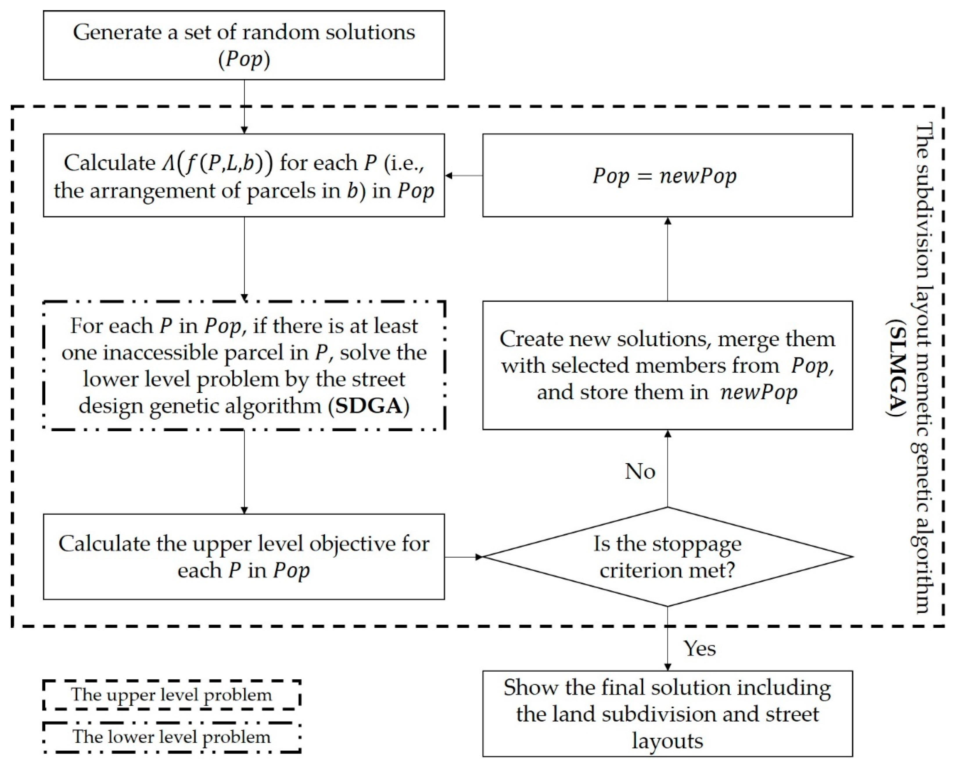
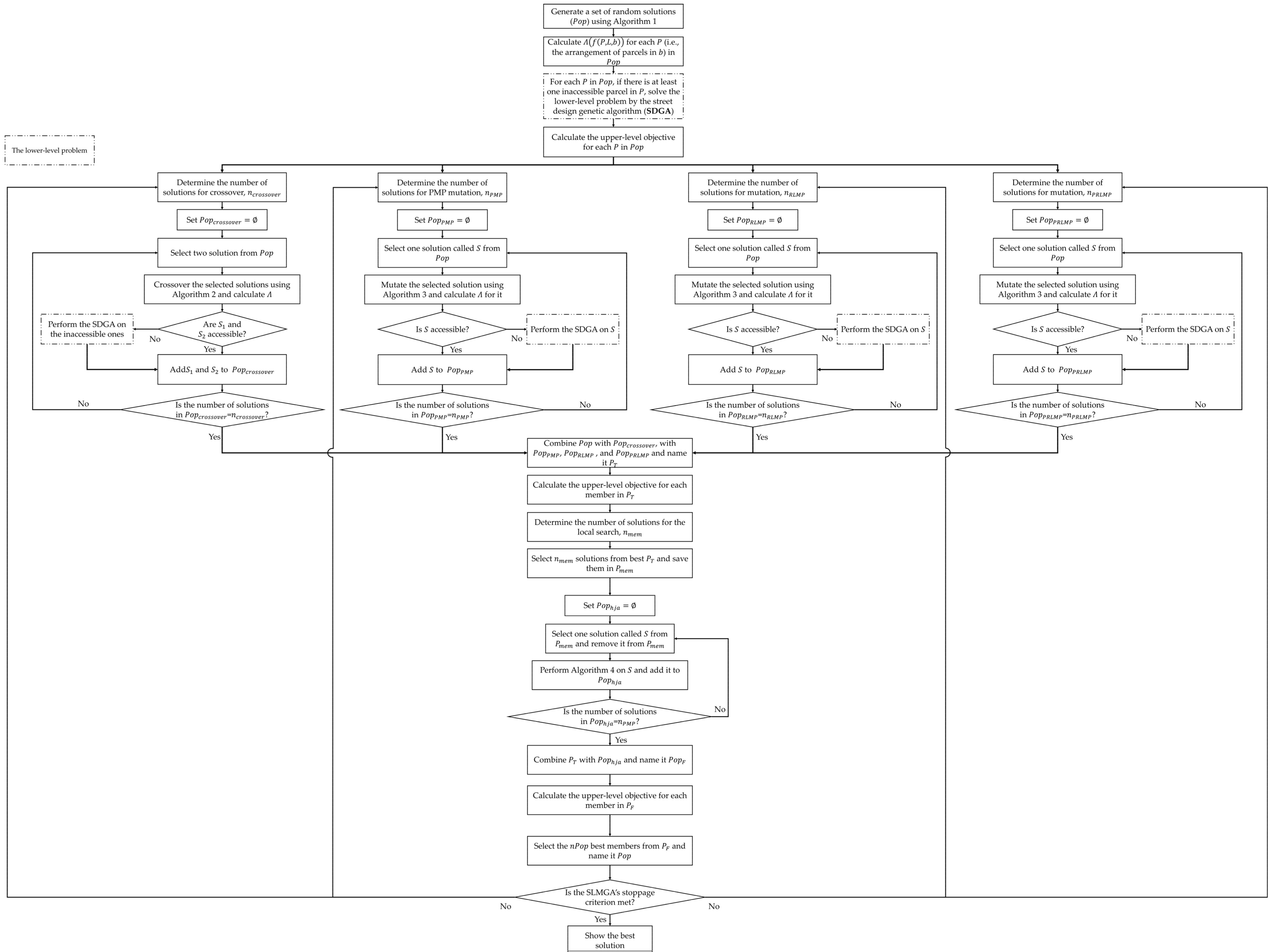
2.2.2. SLMGA Procedure
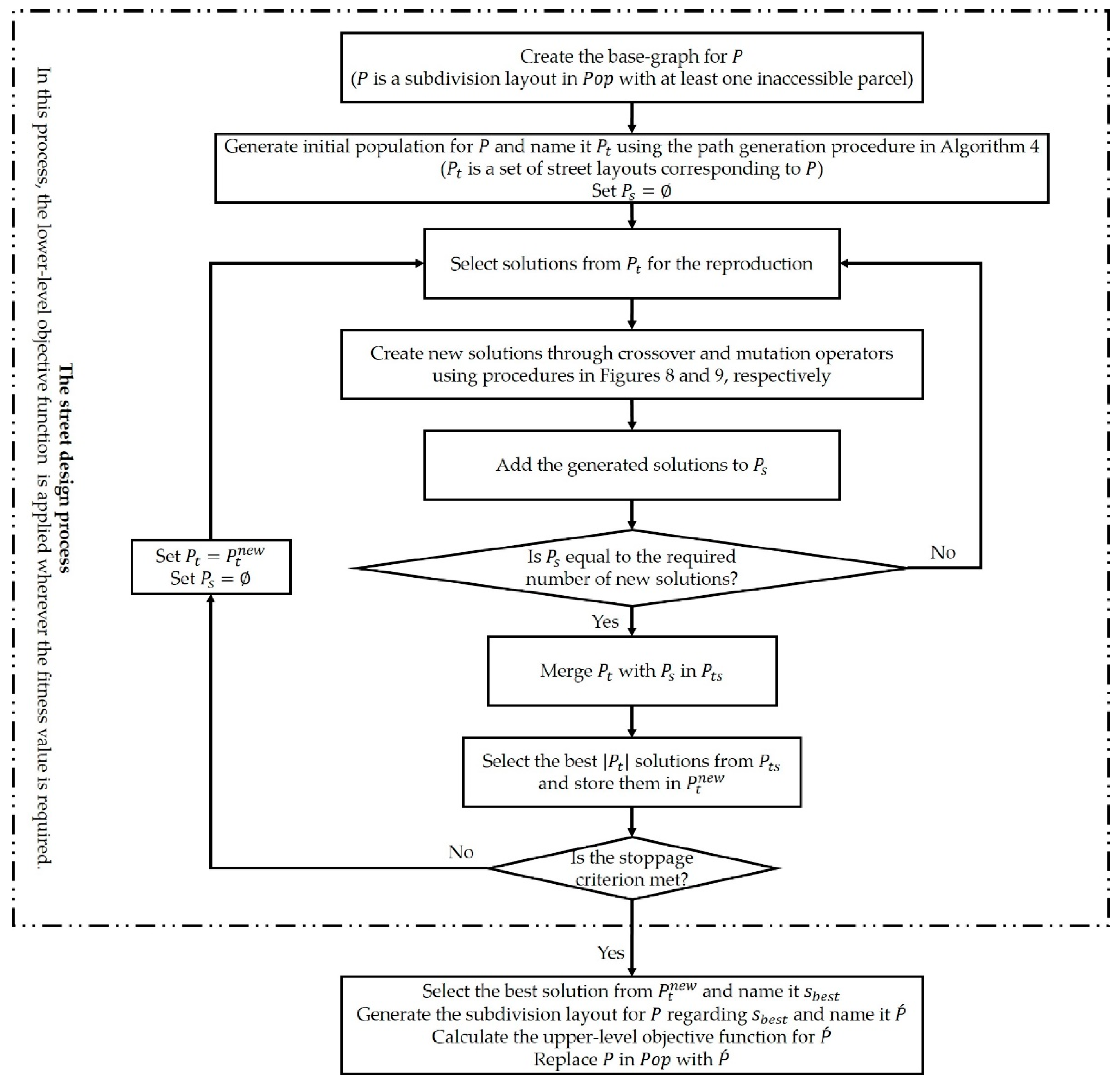
2.2.3. SDGA Procedure
2.3. Case Studies
3. Parameters and Outputs
4. Discussion and Conclusions
Author Contributions
Funding
Data Availability Statement
Acknowledgments
Conflicts of Interest
Appendix A. Details of the Developed and Applied Algorithms
| Algorithm A1: Random Solution Generation Procedure (RSGP) |
| Inputs: |
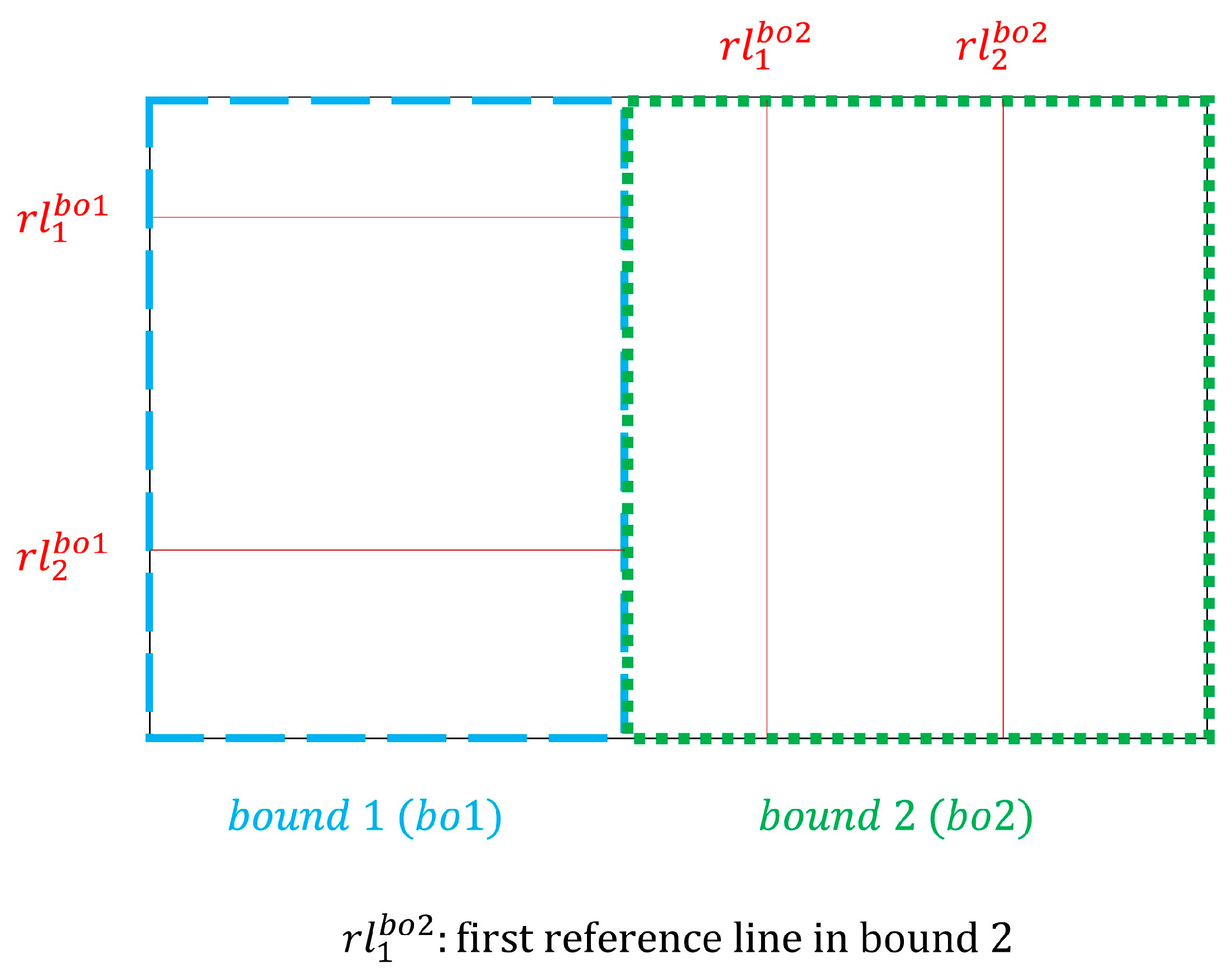
| : The set of reference lines |
| : The number of parcels in a layout |
| : The size of the population |
| Procedure: |
| Set |
| : |
| : |
| : |
| : |
| end if |
| end while |
| end for |
| : |
| ) |
| through the application of Equations (7) and (8) |
| end for |
| : |
| ) |
| through the application of Equations (7) and (8) |
| : |
| through the application of Equations (7) and (8) |
| end while |
| end while |
| end while |
| Algorithm A2: Crossover Procedure |
| Inputs: |
| : The first selected solution |
| : The second selected solution |
| Procedure: |
| and are matched: |
| Create two empty solutions including bounds in and and name them and |
| Transfer reference lines to and |
| Perform the point selection and replacement procedure given , , , and |
| and |
| and ): |
| Create two empty solutions including bounds in and and name them and |
| Perform the reference line selection procedure given and |
| Transfer the reference lines and points inherited from and to and given outputs of the reference line selection procedure |
| Perform the need-capacity calculation procedure given |
| Set |
| : |
| Set |
| Take points from the reference lines of matched with the inherited reference lines in and transfer them to |
| Set |
| Take points from the reference lines of matched with the inherited reference lines in and transfer them to |
| Perform solution repair procedure 1 given |
| Set |
| else: |
| Perform solution repair procedure 2 given |
| Set |
| end if |
| Perform the need-capacity calculation procedure given |
| Set |
| : |
| Set |
| Take points from the reference lines of matched with the inherited reference lines in and transfer them to |
| Set |
| else if : |
| else: |
| end if |
| if : |
| return |
| end if |
| end if |
| Point selection and replacement procedure (PSRP) |
| Inputs: |
| : The first selected solution |
| : The second selected solution |
| : The first off-spring |
| : The second off-spring |
| Procedure: |
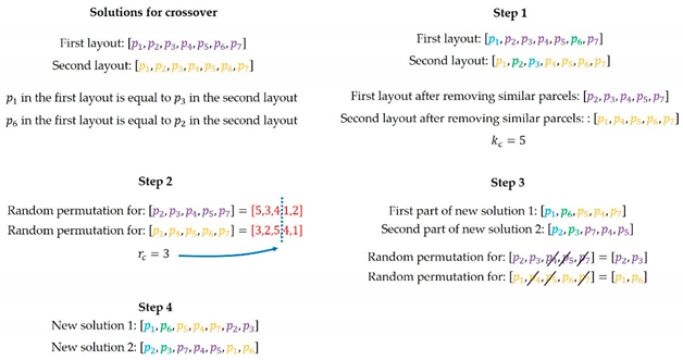
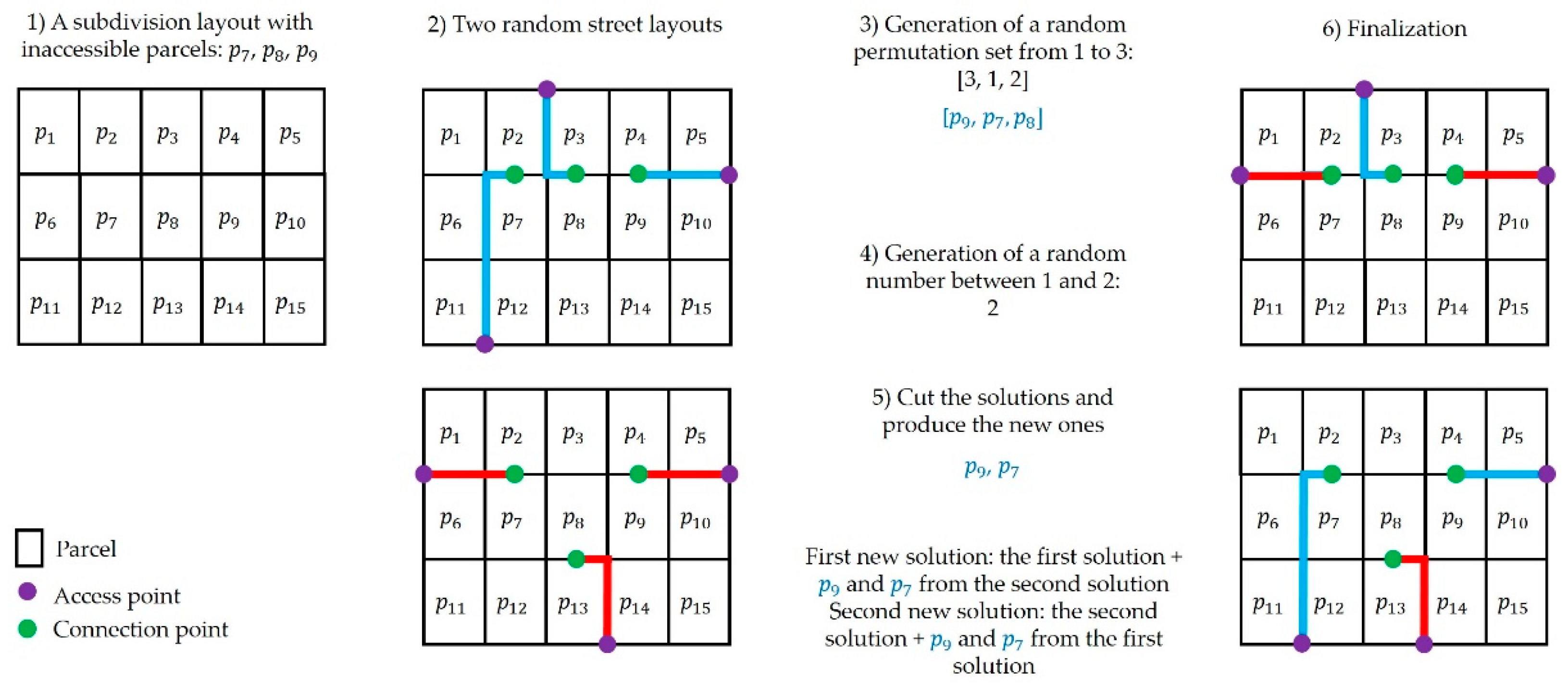
| Assume that and are two lists, including the coordinates of the parcels (e.g., first layout: , and second layout: ). The crossover operator starts with finding and removing parcels with similar coordinates in the two solutions. Then, the PSRP determines the number of remaining parcels denoted by and generates a random permutation for each layout. After that, it produces a cut-off point, , between the number of the remaining parcels in the layouts and . Next, regarding the permutation indices before , the PSRP swaps the remained parcels in the layouts. These parcels and those removed at the beginning of the crossover procedure constitute the first parts of the new solutions. Lastly, the PSRP adds the remaining parcels after to the generated parts, and the off-spring ( and ) are acquired. The figure below displays the PSRP. |
 |
| return populated with parcels |
| Reference line selection procedure (RLSP) |
| Inputs: |
| : The first selected solution |
| : The second selected solution |
| : The first off-spring |
| : The second off-spring |
| Procedure: |
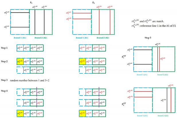
| In the first step, the RLSP arranges reference lines in each bound of sequentially and sorts the bounds in ascending order (). This process is applied to as well (). In the second step, the RLSP identifies and removes the matched reference lines in and . In the third step, it generates a random integer between 1 and the number of remaining reference lines in and . In the fourth step, and are cut and combined. In the last step, the matched reference lines return to and , and the RLSP transfers the reference lines to their corresponding off-spring ( and ). The figure below illustrates the RLSP. |
 |
| return populated with reference lines |
| Need-capacity calculation procedure (NCCP) |
| Inputs: |
| : The first off-spring |
| : The second off-spring |
| Procedure: |
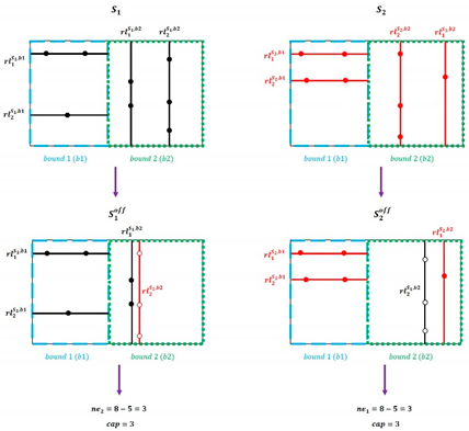
| Given , first, the NCCP counts the number of points on the reference lines inherited from () and calculates the need value () by subtracting from the required number of parcels in the subdivision layout. Second, the NCCP enumerates the number of points on the reference lines inherited from , which is the capacity value () for . Finally, the NCCP returns and . The NCCP is applied to as well. The figure below shows an example of the NCCP application. |
 |
| if is the input: |
| return |
| else if is the input: |
| return |
| end if |
| Solution repair procedure 1 (SRP1) |
| Inputs: |
| : Off-spring |
| : Need value |
| : Capacity value |
| Procedure: |
| if: |
| while : |
| while : |
| end while |
| end while |
| return |
| else if : |
| while : |
| while : |
| end while |
| end while |
| return |
| end if |
| Solution repair procedure 2 (SRP2) |
| Inputs: |
| : Off-spring |
| : Need value |
| Procedure: |
| if: |
| , 4], …]). |
| for: |
| end for |
| while : |
| end while |
| return |
| else if : |
| , 8], …]). |
| for: |
| end for |
| while : |
| end while |
| return |
| end if |
| Algorithm A3: Mutation Procedure |
| Parcel mutation procedure (PMP) |
| Inputs: |
| : The selected solution |
| : The number of parcels in |
| : The number of reference lines in |
| Procedure: |
| Set a random integer between 1 and |
| Select parcels from and store them in |
| Set |
| Store reference lines without parcel in in |
| if : |
| for each in : |
| Select a random reference line from and name it |
| Generate a new coordinate on using Equations (7) and (8) and name it |
| while : |
| Select a random reference line from and name it |
| Generate a new coordinate on using Equations (7) and (8) and name it |
| end while |
| Add to |
| end for |
| else: |
| for each : |
| Generate a new coordinate on using Equations (7) and (8) and name it |
| Add to |
| end for |
| Store parcels in in |
| Set |
| if : |
| for each in : |
| Select a random reference line from and name it |
| Generate a new coordinate on using Equations (7) and (8) and name it |
| while : |
| Select a random reference line from and name it |
| Generate a new coordinate on using Equations (7) and (8) and name it |
| end while |
| Add to |
| end for |
| end if |
| end if |
| return |
| Reference line mutation procedure (RLMP) |
| Inputs: |
| : The selected solution |
| : The number of parcels in |
| : The number of reference lines in |
| Procedure: |
| Generate a random number between 1 and and name it |
| Select reference lines from randomly and store them in |
| Set |
| for each in : |
| Create a random point within the bound corresponding to in a way that the point does not intersect with another reference line and name it |
| Create a new reference line passing through and parallel to and name it |
| Project points on onto using the parcel projection procedure (PPP) that keeps the proportion of distances between points on the same as |
| Add to |
| Remove from |
| end for |
| Parcel Projection Procedure (PPP) |
| Inputs: |
| : The main reference line |
| : The new reference line |
| Procedure: |
| Set as the start point of |
| Set as the end point of |
| Set as the beginning point of |
| Set as the last point of |
| Set as the line connecting to |
| Set as the line connecting to |
| if intersects : |
| Set |
| Set |
| else: |
| Set |
| Set |
| end if |
| Set |
| for each on : |
| Set as the distance between and |
| Set |
| Set as the circle with center of and radius of |
| Set as the intersection between and |
| Add to |
| end for |
| Set points in on |
| Parcel and reference line mutation procedure (PRLMP) |
| Inputs: |
| : The selected solution |
| Procedure: |
| Perform RLMP on and name it |
| Perform PMP on and name it |
| return |
| Algorithm A4: Hooke and Jeeves Procedure |
| Inputs: |
| : The selected solution |
| : The vector including distances for the exploratory search |
| : The vector including termination values for each parcel |
| Procedure: |
| : |
| is acceptable: |
| using Equation (14) |
| is acceptable: |
| is acceptable: |
| : |
| is acceptable: |
| is not acceptable: |
| end if |
| else: |
| end while |
| else: |
| else: |
| else: |
| end while |
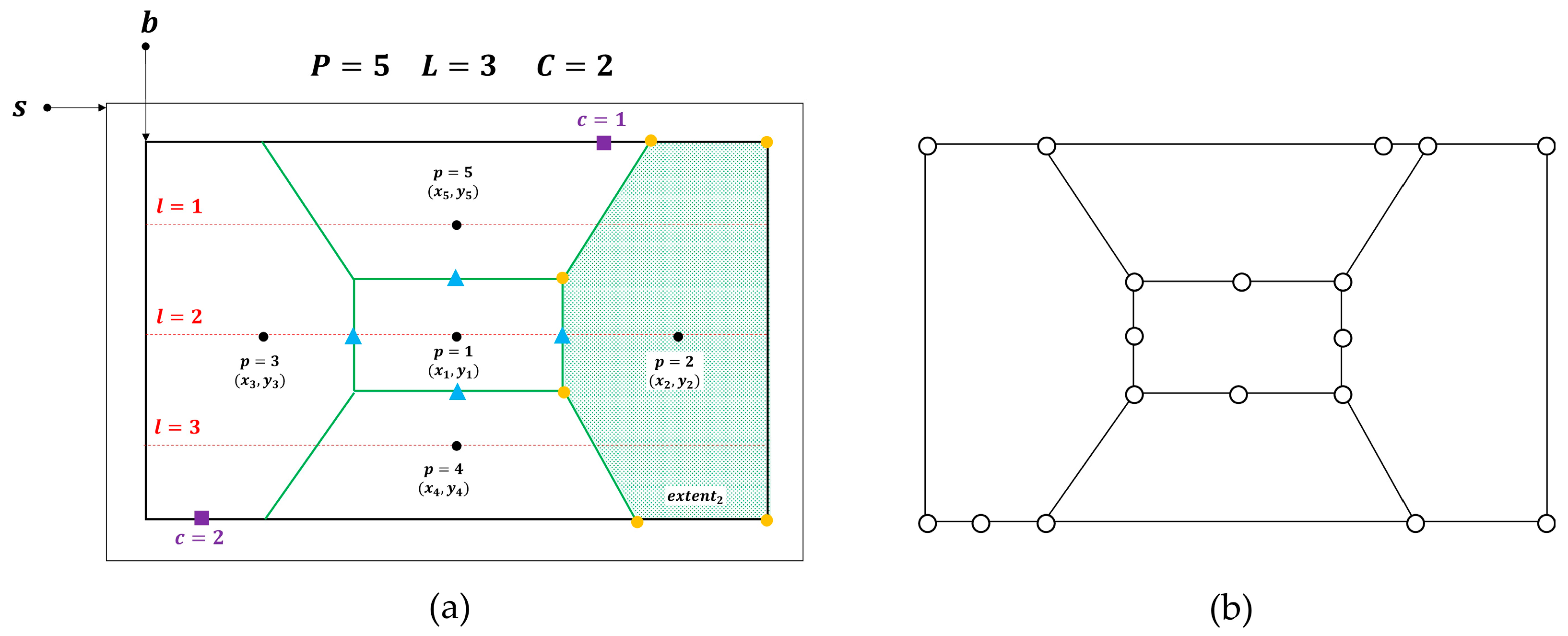
| Algorithm A5: Graph Generation Procedure for a Subdivision Layout (GGP) |
| Inputs: |
| : The set of parcels |
| : The set of access points |
| : The set of connection rules |
| Procedure: |
| as the access point |
| : |
| and mark each point with the parcels it is on the edge of |
| end for |
| Connect N to M |
| , a connected network in which connection and access points are marked, and each link is separated from the point entities on them |
| Algorithm A6: Population Generation Procedure for the SDGA |
| Inputs: |
| : The set of parcels |
| : The set of inaccessible parcels |
| : The set of access points |
| Procedure: |
| : |
| : |
| : |
| end if |
| end for |
| end while |
| Path creation procedure |
| Inputs: |
| : The connection point or origin |
| : The access point or destination |
| : The base-graph |
| Procedure: |
| Perform Dijkstra’s shortest path algorithm [45] given cc, c, RLC, and G(N‚M) |
| return the path generated by the Dijkstra’s algorithm |
References
- Sonnenberg, J. Fundamentals of land consolidation as an instrument to abolish fragmentation of agricultural holdings. In Proceedings of the FIG XXII International Congress, Washington, DC, USA, 19–26 April 2002. [Google Scholar]
- Demetriou, D.; See, L.; Stillwell, J. A spatial genetic algorithm for automating land partitioning. Int. J. Geogr. Inf. Sci. 2013, 27, 2391–2409. [Google Scholar] [CrossRef]
- Stevens, D.; Dragićević, S. A GIS-based irregular cellular automata model of land-use change. Environ. Plan. B Plan. Des. 2007, 34, 708–724. [Google Scholar] [CrossRef]
- Wakchaure, A.S. An ArcView Tool for Simulating Land Subdivision for Build Out Analysis. Master’s Thesis, Faculty of Virginia Polytechnic Institute and State University, Blacksburg, VN, USA, 2001. [Google Scholar]
- Habib, M. Proposed Algorithm of Land Parcel Subdivision. J. Surv. Eng. 2020, 146, 04020012. [Google Scholar] [CrossRef]
- Buis, A.; Vingerhoeds, R.A. Knowledge-based systems in the design of a new parcelling. Knowl.-Based Syst. 1996, 9, 307–314. [Google Scholar] [CrossRef]
- Parish, Y.I.; Müller, P. Procedural modeling of cities. In Proceedings of the 28th Annual Conference on Computer Graphics and Interactive Techniques, Los Angeles, CA, USA, 12–17 August 2001; pp. 301–308. [Google Scholar]
- Touriño, J.; Parapar, J.; Doallo, R.; Boullón, M.; Rivera, F.F.; Bruguera, J.D.; Gonzalez, X.P.; Crecente, R.; Álvarez, C. A GIS-embedded system to support land consolidation plans in Galicia. Int. J. Geogr. Inf. Sci. 2003, 17, 377–396. [Google Scholar] [CrossRef]
- Halatsch, J.; Kunze, A.; Schmitt, G. Using shape grammars for master planning. In Design Computing and Cognition’08; Springer: Berlin/Heidelberg, Germany, 2008; pp. 655–673. [Google Scholar]
- Marshall, S. Cities, Design and Evolution; Routledge: London, UK, 2009. [Google Scholar]
- Vanegas, C.A.; Aliaga, D.G.; Benes, B.; Waddell, P. Visualization of simulated urban spaces: Inferring parameterized generation of streets, parcels, and aerial imagery. IEEE Trans. Vis. Comput. Graph. 2009, 15, 424–435. [Google Scholar] [CrossRef] [PubMed]
- Vanegas, C.A.; Aliaga, D.G.; Benes, B.; Waddell, P.A. Interactive design of urban spaces using geometrical and behavioral modeling. ACM Trans. Graph. 2009, 28, 1–10. [Google Scholar] [CrossRef]
- Vanegas, C.A.; Kelly, T.; Weber, B.; Halatsch, J.; Aliaga, D.G.; Müller, P. Procedural generation of parcels in urban modeling. Comput. Graph. Forum 2012, 31, 681–690. [Google Scholar] [CrossRef]
- Engine, C. Esri City Engine Documentation—Block Parameters Module. Available online: https://doc.arcgis.com/en/cityengine/latest/help/help-layers-block-parameters.htm (accessed on 20 May 2024).
- Colomb, M.; Tannier, C.; Perret, J.; Chapron, P.; Brasebin, M. Parcel Manager: A parcel reshaping model incorporating design rules of residential development. Trans. GIS 2022, 26, 2558–2597. [Google Scholar] [CrossRef]
- Wickramasuriya, R.; Chisholm, L.A.; Puotinen, M.; Gill, N.; Klepeis, P. An automated land subdivision tool for urban and regional planning: Concepts, implementation and testing. Environ. Model. Softw. 2011, 26, 1675–1684. [Google Scholar] [CrossRef]
- Dahal, K.R.; Chow, T.E. A GIS toolset for automated partitioning of urban lands. Environ. Model. Softw. 2014, 55, 222–234. [Google Scholar] [CrossRef]
- Demetriou, D.; Stillwell, J.; See, L.M. LandParcelS: A Module for Automated Land Partitioning; School of Geography, University of Leeds: Leeds, UK, 2012. [Google Scholar]
- Hillier, F.S.; Lieberman, G.J. Introduction to Operations Research; McGraw-Hill Higher Education: New York, NY, USA, 2010. [Google Scholar]
- Haklı, H.; Uğuz, H.; Çay, T. A new approach for automating land partitioning using binary search and Delaunay triangulation. Comput. Electron. Agric. 2016, 125, 129–136. [Google Scholar] [CrossRef]
- Koc, I.; Cay, T.; Babaoglu, I. Approaches to automated land subdivision using binary search algorithm in zoning applications. Proc. Inst. Civ. Eng. Munic. Eng. 2022, 175, 16–28. [Google Scholar] [CrossRef]
- Kucukmehmetoglu, M.; Geymen, A. Optimization models for urban land readjustment practices in Turkey. Habitat Int. 2016, 53, 517–533. [Google Scholar] [CrossRef]
- Koc, I.; Cay, T.; Babaoglu, I. A novel metaheuristic algorithm by efficient crossover operator for land readjustment. Expert Syst. Appl. 2022, 188, 116082. [Google Scholar] [CrossRef]
- Mustafa, A.; Wei Zhang, X.; Aliaga, D.G.; Bruwier, M.; Nishida, G.; Dewals, B.; Erpicum, S.; Archambeau, P.; Pirotton, M.; Teller, J. Procedural generation of flood-sensitive urban layouts. Environ. Plan. B Urban Anal. City Sci. 2020, 47, 889–911. [Google Scholar] [CrossRef]
- Yang, Y.-L.; Wang, J.; Vouga, E.; Wonka, P. Urban pattern: Layout design by hierarchical domain splitting. ACM Trans. Graph. 2013, 32, 1–12. [Google Scholar] [CrossRef]
- Hejazi, S.R.; Memariani, A.; Jahanshahloo, G.; Sepehri, M.M. Linear bilevel programming solution by genetic algorithm. Comput. Oper. Res. 2002, 29, 1913–1925. [Google Scholar] [CrossRef]
- Miandoabchi, E.; Daneshzand, F.; Szeto, W.Y.; Farahani, R.Z. Multi-objective discrete urban road network design. Comput. Oper. Res. 2013, 40, 2429–2449. [Google Scholar] [CrossRef]
- Wang, Z.; Han, Q.; de Vries, B. Land use oriented bi-level discrete road network design. Transp. Res. Procedia 2019, 37, 35–42. [Google Scholar] [CrossRef]
- Xu, T.; Wei, H.; Hu, G. Study on continuous network design problem using simulated annealing and genetic algorithm. Expert Syst. Appl. 2009, 36, 1322–1328. [Google Scholar] [CrossRef]
- Kennedy, J.; Eberhart, R. Particle swarm optimization. In Proceedings of the ICNN’95-International Conference on Neural Networks, Perth, WA, Australia, 27 November–1 December 1995; pp. 1942–1948. [Google Scholar]
- Sahebgharani, A. Multi-objective Land Use Optimizarion through Parallel Particle Swarm Algorithm: Cade Study Baboldasht District of Isfahan, Iran. J. Urban Environ. Eng. 2016, 10, 42–49. [Google Scholar] [CrossRef]
- Kirkpatrick, S.; Gelatt, C.D., Jr.; Vecchi, M.P. Optimization by simulated annealing. Science 1983, 220, 671–680. [Google Scholar] [CrossRef] [PubMed]
- Mohammadi, M.; Nastaran, M.; Sahebgharani, A. Development, application, and comparison of hybrid meta-heuristics for urban land-use allocation optimization: Tabu search, genetic, GRASP, and simulated annealing algorithms. Comput. Environ. Urban Syst. 2016, 60, 23–36. [Google Scholar] [CrossRef]
- Dorigo, M. Optimization, Learning and Natural Algorithms. Ph.D. Thesis, Politecnico di Milano, Milan, Italy, 1992. [Google Scholar]
- Liu, X.; Li, X.; Shi, X.; Huang, K.; Liu, Y. A multi-type ant colony optimization (MACO) method for optimal land use allocation in large areas. Int. J. Geogr. Inf. Sci. 2012, 26, 1325–1343. [Google Scholar] [CrossRef]
- Cao, K.; Liu, M.; Wang, S.; Liu, M.; Zhang, W.; Meng, Q.; Huang, B. Spatial multi-objective land use optimization toward livability based on boundary-based genetic algorithm: A case study in Singapore. ISPRS Int. J. Geo-Inf. 2020, 9, 40. [Google Scholar] [CrossRef]
- Holland, J.H. Adaptation in Natural and Artificial Systems; University of Michigan Press: Ann Arbor, MI, USA, 1975. [Google Scholar]
- Alam Tabriz, A.; Zandieh, M.; Mohammad Rahimi, A. Metaheuristic Algorithms in Combinatorial Optimization; Saffar Publications: Harvey, IL, USA, 2013. [Google Scholar]
- Fattahi, P. Metaheuristic Algorithms; Bu-Ali Sina University: Hamedan, Iran, 2011. [Google Scholar]
- Sivanandam, S.; Deepa, S. Genetic algorithms. In Introduction to Genetic Algorithms; Springer: Berlin/Heidelberg, Germany, 2008; pp. 15–37. [Google Scholar]
- Hamidizadeh, M.R. Nonlinear Programming; Samt Publication: Tehran, Iran, 2022. [Google Scholar]
- Chen, B.Y.; Lam, W.H.; Sumalee, A.; Li, Q.; Shao, H.; Fang, Z. Finding reliable shortest paths in road networks under uncertainty. Netw. Spat. Econ. 2013, 13, 123–148. [Google Scholar] [CrossRef]
- Khalili-Damghani, K.; Aminzadeh-Goharrizi, B.; Rastegar, S.; Aminzadeh-Goharrizi, B. Solving land-use suitability analysis and planning problem by a hybrid meta-heuristic algorithm. Int. J. Geogr. Inf. Sci. 2014, 28, 2390–2416. [Google Scholar] [CrossRef]
- Sahebgharani, A.; Haghshenas, H.; Mohammadi, M. Reliable Space-Time Prisms in the Stochastic Road Networks Under Spatial Correlated Travel Times. Transp. B Transp. Dyn. 2020, 8, 351–375. [Google Scholar]
- Dijkstra, E.W. A note on two problems in connexion with graphs. Numer. Math. 1959, 1, 269–271. [Google Scholar] [CrossRef]

| Case Number | Subdivision Area | Requirements |
|---|---|---|
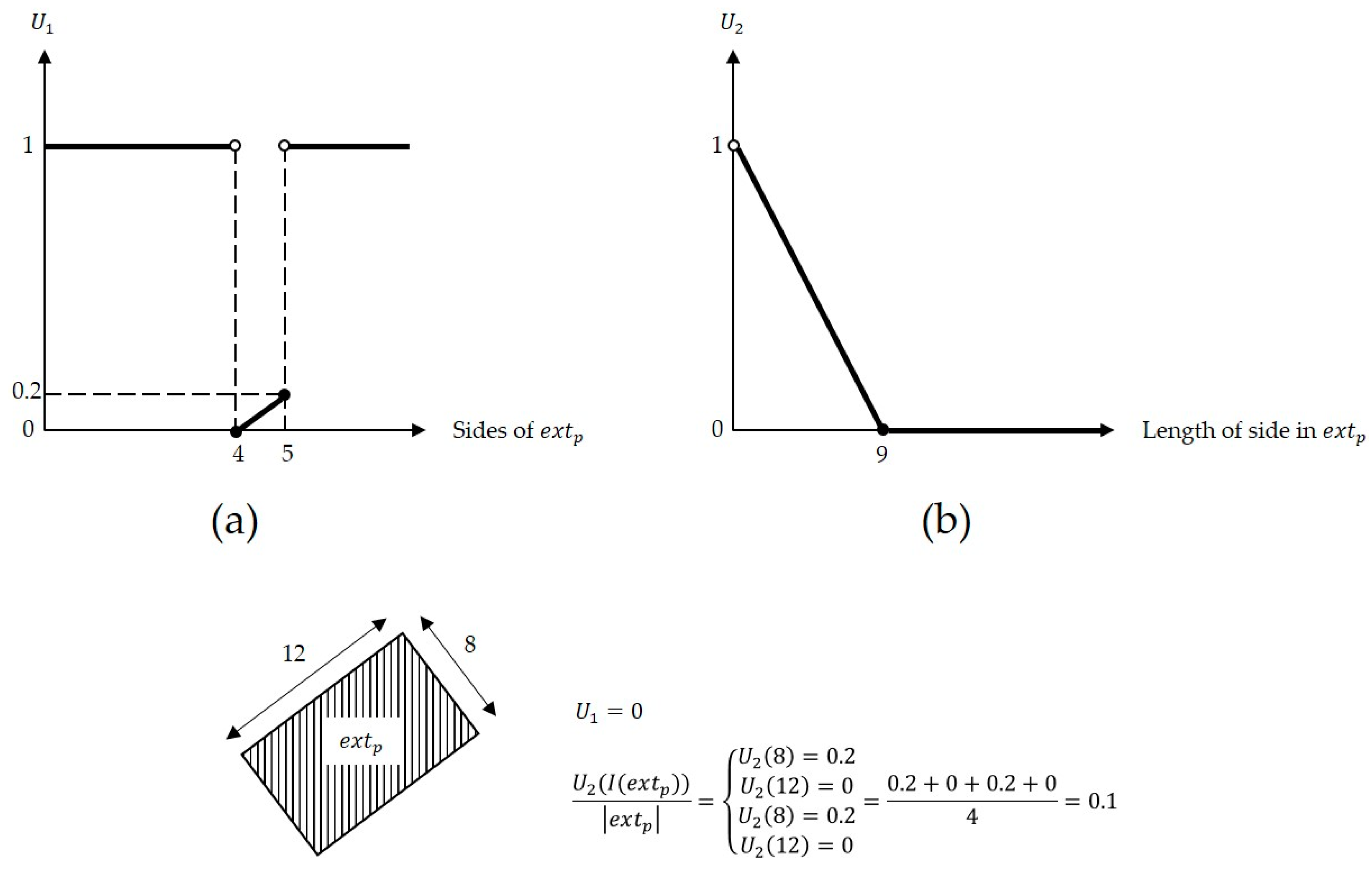
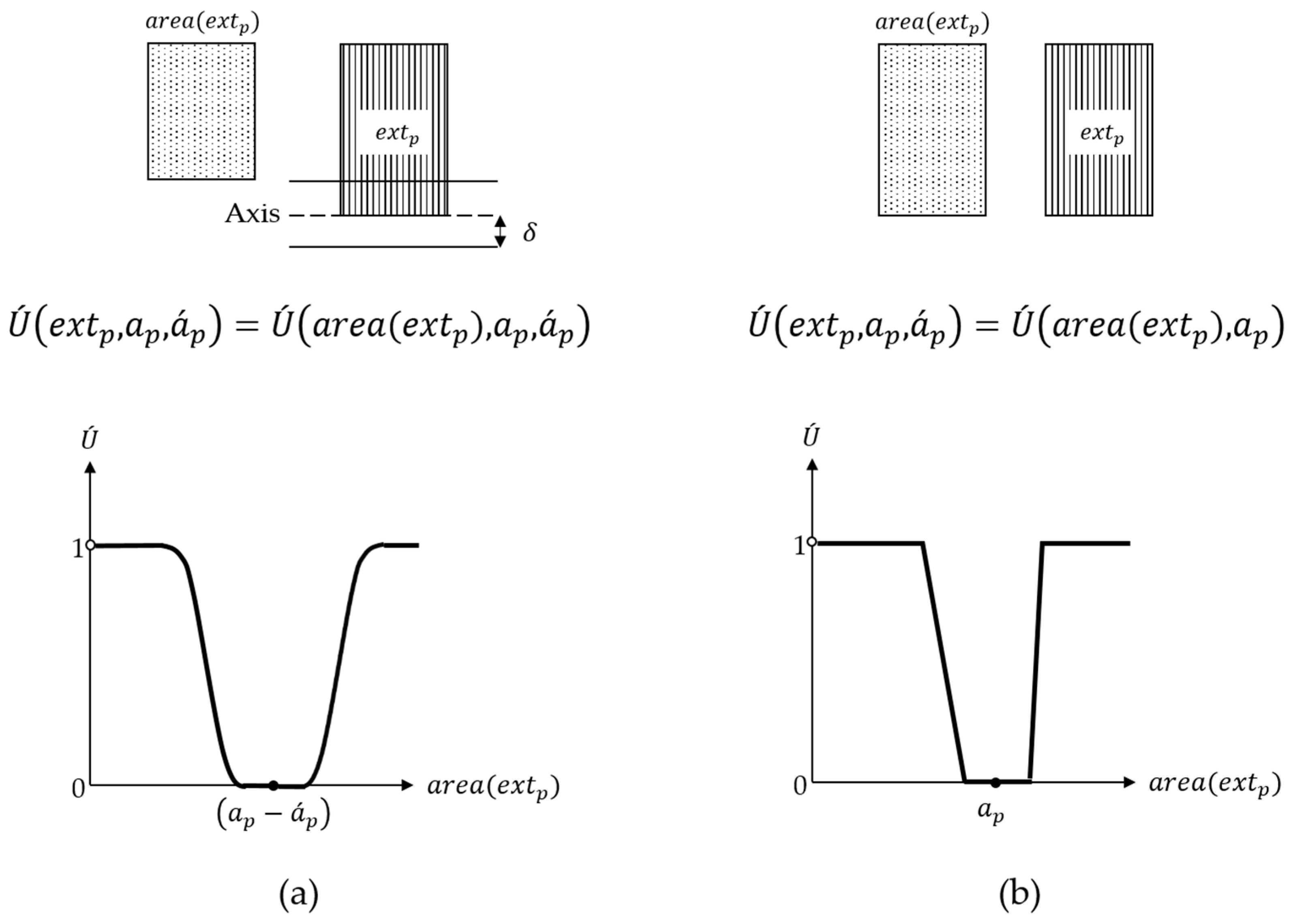
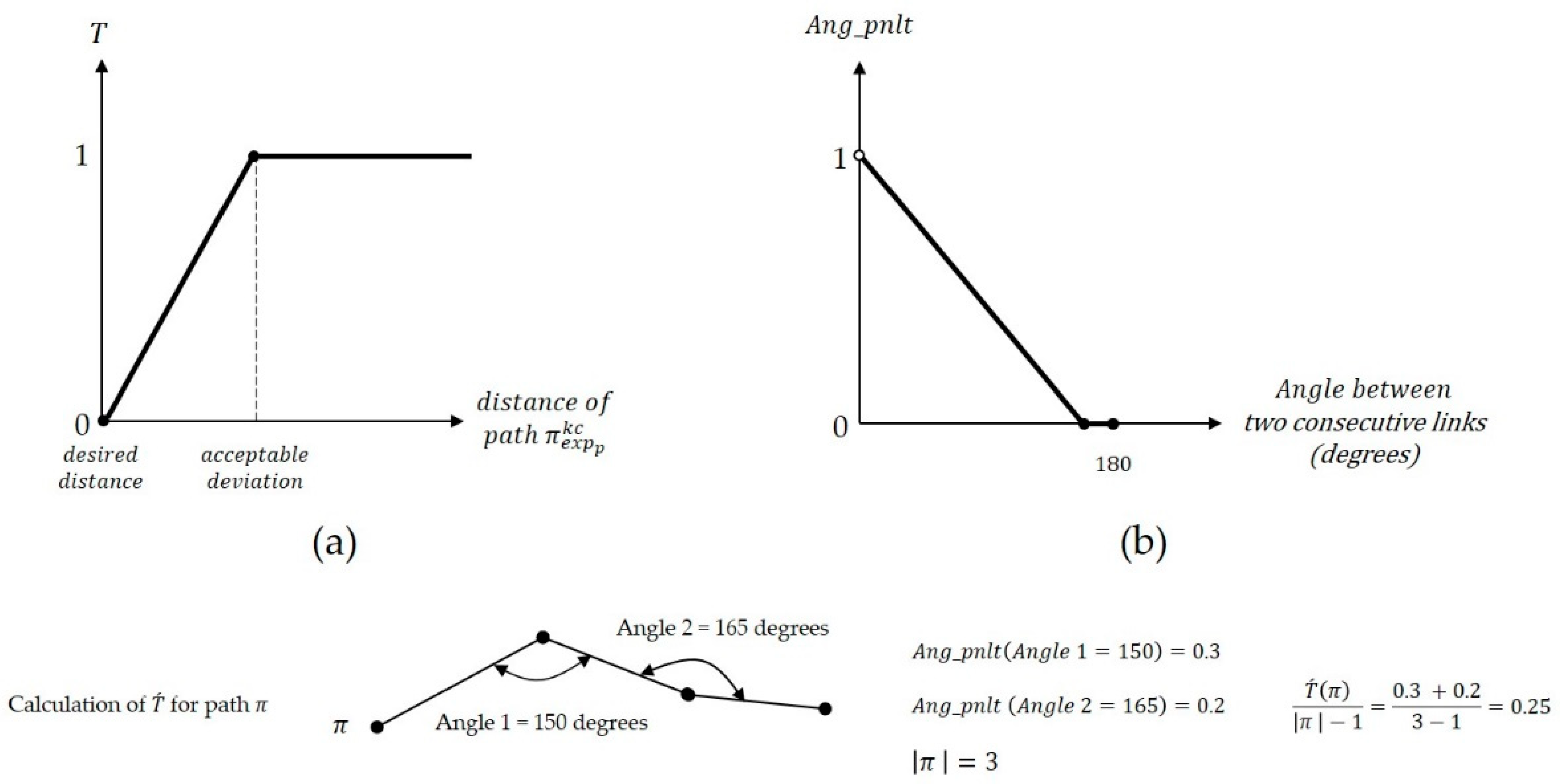
| C1 | 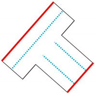 | R1: Inaccessible parcels can be connected through the midpoint of their sides. R2: 8 m. R3: 34. . R5: Weights of the parcel’s number of sides (). R6: U1 is the same as the function in Figure 2a. U2 is like the function in Figure 2b, but 2 replaces 9 on the horizontal axis. R7: The form of the function is like Figure 3b. Cut-off points on the horizontal axis are . R8: Street evaluation functions are the same as Figure 4a,b. The cut-off for T is 60. The first and second points on the horizontal axis of are 150 and 180, respectively. R9: . R10: Thirty-four parcels with an area of 100 square meters are required. General comments on the layout: Three reference lines marked in blue are considered, and the accessibility of the block is provided through the red line. Note that values for the area and length are dimensionless. In addition, it is assumed that other context-specific factors have been controlled for analysis purposes. |
| C2 | 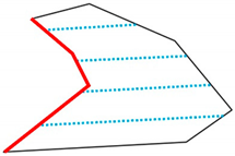 | R1: Inaccessible parcels can be connected through the midpoint of their sides. R2: 8 m. R3: 10. R4: . R5: Weights of the parcel’s number of sides (). R6: U1 is the same as the function in Figure 2a. U2 is like the function in Figure 2b, but 5 replaces 9 on the horizontal axis. R7: The form of the function is like Figure 3b. Cut-off points on the horizontal axis are . R8: Street evaluation functions are the same as Figure 4a,b. The cut-off for T is 20. The first and second points on the horizontal axis of are 150 and 180, respectively. R9: . R10: Ten parcels with areas of 600, 500, 400, 600, 1000, 400, 1000, 5000, 1000, and 462.5 square meters are required. General comments on the layout: Four reference lines marked in blue are considered, and the accessibility of the block is provided through the red line. Note that values for the area and length are dimensionless. In addition, it is assumed that other context-specific factors have been controlled for analysis purposes. |
| Parameter † | Value | Parameter | Value |
|---|---|---|---|
| Crossover probability () | 0.8 | Iteration | 200 |
| Mutation probability () | 0.9 | HJV exploratory search parameter () | 0.5 |
| Population size () | 200 | HJV termination parameter () | 0.0001 |
| Case Number | Algorithm Output | Planner Output |
|---|---|---|
| C1 | 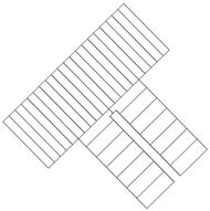 | 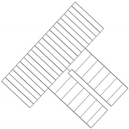 |
| C2 | 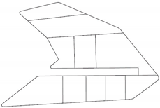 |  |
| Indicator | C1 | C2 | |
|---|---|---|---|
| Objective value | p-value | 0.844 | 0.322 |
| t-value | −0.198 | −1.008 | |
| Solution time | p-value | 0.973 | 0.898 |
| t-value | −0.034 | −1.290 | |
Disclaimer/Publisher’s Note: The statements, opinions and data contained in all publications are solely those of the individual author(s) and contributor(s) and not of MDPI and/or the editor(s). MDPI and/or the editor(s) disclaim responsibility for any injury to people or property resulting from any ideas, methods, instructions or products referred to in the content. |
© 2024 by the authors. Licensee MDPI, Basel, Switzerland. This article is an open access article distributed under the terms and conditions of the Creative Commons Attribution (CC BY) license (https://creativecommons.org/licenses/by/4.0/).
Share and Cite
Sahebgharani, A.; Wiśniewski, S. Developing a Bi-Level Optimization Model for the Coupled Street Network and Land Subdivision Design Problem with Various Lot Areas in Irregular Blocks. ISPRS Int. J. Geo-Inf. 2024, 13, 224. https://doi.org/10.3390/ijgi13070224
Sahebgharani A, Wiśniewski S. Developing a Bi-Level Optimization Model for the Coupled Street Network and Land Subdivision Design Problem with Various Lot Areas in Irregular Blocks. ISPRS International Journal of Geo-Information. 2024; 13(7):224. https://doi.org/10.3390/ijgi13070224
Chicago/Turabian StyleSahebgharani, Alireza, and Szymon Wiśniewski. 2024. "Developing a Bi-Level Optimization Model for the Coupled Street Network and Land Subdivision Design Problem with Various Lot Areas in Irregular Blocks" ISPRS International Journal of Geo-Information 13, no. 7: 224. https://doi.org/10.3390/ijgi13070224
APA StyleSahebgharani, A., & Wiśniewski, S. (2024). Developing a Bi-Level Optimization Model for the Coupled Street Network and Land Subdivision Design Problem with Various Lot Areas in Irregular Blocks. ISPRS International Journal of Geo-Information, 13(7), 224. https://doi.org/10.3390/ijgi13070224