Abstract
This paper describes the use of Generalized Additive Models (GAMs) to create regression models whose coefficient estimates vary with geographic location—spatially varying coefficient (SVC) models. The approach uses Gaussian Process (GP) splines (smooths) for each predictor variable, which are parameterised with observation location in order to generate SVC estimates. These describe the spatially varying relationships between predictor and response variables. The proposed GAM approach was compared with Multiscale Geographically Weighted Regression (MGWR) using simulated data with complex spatial heterogeneities. The geographical GP GAM (GGP-GAM) was found to out-perform MGWR across a range of fit metrics and resulted in more accurate coefficient estimates and lower residual errors. One of the GGP-GAM models was investigated in detail to illustrate model diagnostics, checks of spline/smooth convergence and basis evaluations. A larger simulated case study was investigated to explore the trade-offs between GGP-GAM complexity (via the number of knots), performance and computational efficiency. Finally, the GGP-GAM and MGWR approaches were applied to an empirical case study. The resulting models had very similar accuracies and fits and generated subtly different spatially varying coefficient estimates. A number of areas of further work are identified.
1. Introduction
In regression, the relationship between response and predictor variables may vary with observation location. This may be due to a poor conceptual model; poor measurements with regional biases; omitted local factors or the presence of process spatial heterogeneity, also known as process spatial non-stationarity. In such cases, spatially varying coefficient (SVC) models provide an alternative to global or whole-map regressions, in which the relationships between response and predictor variables are assumed to be constant across space by relaxing the assumption of relationship spatial stationarity [1]. SVC models allow relationships to vary with observation location and generate spatially distributed or local coefficient estimates. These quantify process spatial non-stationarity or spatial heterogeneity—a key and increasingly common task in spatial data analysis—and can be mapped to indicate how and where statistical relationships vary. SVCs provide insights into the spatially varying natures of different drivers of a response and can guide further investigations.
The SVC brand leader is Geographically Weighted Regression (GWR) [2], which uses a single moving window or kernel whose size is optimised and determines the scale of spatial heterogeneity in the resultant outputs. GWR has been extended to a multiscale approach (MGWR) [3,4] in which individual kernels are fitted for each predictor variable, thereby capturing individual scales of the spatially varying relationships between predictor and response variables. MGWR is considered by some to be the default GWR model [5]. However, there are a number of limitations associated with MGWR approaches, the main ones being that they cannot predict out of sample and that only approaches for Gaussian and Poisson responses have been developed [6].
This paper addresses these critical gaps and describes a novel SVC modelling approach that uses Generalized Additive Models (GAMs) [7,8] with Gaussian Process (GP) smooths to capture process spatial non-stationarity. GAM smooths are commonly used to accommodate varying relationships between predictor and response variables in attribute space. But if the smooths are parameterised with observation location, then the result is an SVC, as the relationship between the target variable and each predictor is estimated locally over geographic space. The GAM-based SVC approach proposed in this paper—the Geographical Gaussian Process GAM (GGP-GAM)—is evaluated through three experiments. The first compares it with MGWR using simulated data with complex and highly localised degrees of spatial heterogeneity. Both models are fully tuned. The second investigates the ability of GGP-GAM to handle larger datasets and examines how performance is affected as the number of knots used in the smooths increases. Finally, an empirical case study of the UK referendum to leave the European Union in 2016 (Brexit) is used illustrate and compare MGWR and GAM-based approaches.
2. Literature Review
2.1. SVC Models
Spatially varying coefficient regression models seek to the capture spatial dependencies in each relationship between target and predictor variables. Their outputs provide explicit indications of the scales of these and their spatial variations. A widely used SVC model is geographically weighted regression (GWR) [2], which has been extended to Multiscale GWR (MGWR) [3,4]. In a MGWR/GWR, a series of local models is created using data subsets extracted using a moving window or kernel. For each local model, the subset data are weighted by their distance to the location under consideration, resulting in local, spatially distributed coefficient estimates. Kernel size is optimised using a weighted least squares algorithm or AIC in a standard GWR and an iterative back-fitting algorithm in MGWR. Besides GWR/MGWR, other widely utilized multiscale SVC models include Bayesian Gaussian Process (GP) models that employ co-kriging via a Linear Model of Co-regionalisation (LMC) (Bayes-GP) [9,10,11,12] and Eigenvector Spatial Filtering (ESF) with Moran coefficients (ESF-MC) [13,14,15]. ESF-MC enhances the deterministic ESF model [16] by incorporating random effects to capture stochastic spatial processes. These SVC models are directly inter-related [15], and comparative analyses indicate that no single multiscale SVC model is significantly better than others. Recently, other multiscale SVC models have emerged, such as a triangulation model utilizing bivariate spline estimators [17], a GP-based model adopting a frequentist approach with ML estimation [18] and a GLM-based model incorporating a reduced-rank spline [19]. However, these SVC models have not been widely adopted by the research community, and the use of GWR approaches has increased rapidly [20]. However, there are a number of theoretical limitations associated with GWR approaches (including MGWR): they generate a collection of local models rather than a single one, while Bayes-GP, ESF-MC and GGP-GAM each offer a single, non-stationary model formulation (e.g., [10,21]); the same observation is used in multiple local models; and MGWR approaches cannot predict out of sample. As a result, it has been argued that GWR and MGWR are essentially exploratory approaches [18,22].
2.2. GAM-Based SVC Models
GAMs can handle different types of response variables and produce multiple model terms that are additively combined [7,8,23]. In this way, they capture complex data relationships and interactions, including non-linearities between predictor and response variables [24]. GAMs provide a framework for making predictions from complex systems, for quantifying variable relationships and for making inferences about these relationships [7,8]. They perform as well as many machine learning models in terms of prediction accuracy and computational speed [25], and critically, in the context of varying coefficient modelling, GAMs combine this inferential power with transparency and process understanding. They have been described as providing “intrinsically understandable white-box machine learning models that provide a technically equivalent, but ethically more acceptable alternative to [machine learning] black-box models” ([26], p. 2).
GAMs can incorporate smooths or splines to model non-linear relationships, whose forms can vary depending on the problem and/or the data [8]. Smooths are composed of combinations of basis functions that can be single- or multi-dimensional in terms of predictor variables. Consequently, GAMs with smooths are composed of sums of multiple basis functions and, in this way, are able to model complex data relationships. As a result of these properties, a number varying coefficient and Bayesian regression models using GAMs have been proposed [27,28,29,30]. These make few assumptions about the response variable distribution (which may be skewed, kurtotic or discrete), and their ‘varying coefficient’ aspects relate to the target variable properties of location, scale and shape. ‘Location’ refers to the central tendencies of the target variable, ‘scale’ to measures of spread such as standard deviation in normal distributions and ‘shape’ to the nature of the skew and kurtosis in the distribution. Thus, such GAM-based varying coefficient approaches accommodate ‘spatial’ effects but not within an explicitly geographic framework with respect to location. Recent work proposed an SVC GLM regression model using GAMs [19] with reduced-rank, thin-plate smooths; however, an alternative approach for modelling predictor-to-response relationships is to consider them as Gaussian processes (GPs) over space. GPs capture relationships that decay over distance, reflecting Tobler’s First Law of Geography [31] and have been found to be effective in handling spatial autocorrelation [32]. The approach proposed in this paper uses decomposed or low-rank GP smooths parameterised with observation location for each predictor variable. It extends initial investigations of GAMs in SVC modelling using the geographical Gaussian process GAM (GGP-GAM) [33] by exploring GAM tuning with more complex spatial problems.
3. Methodology
Three analyses were undertaken. The first compared GGP-GAM and MGWR SVC models of 100 simulated datasets, each with 625 observations, a target variable (y) and 3 predictor variables (, and ). A second set of analyses investigated the ability of the GAM approach to handle larger datasets—in this case, with 250,000 observations—and model tuning via the knots parameter (k). The aim was to identify possible trade-offs between model performance, accuracy and computational cost. A third analysis compared GGP-GAM and MGWR using an empirical case study of the Brexit vote in the UK.
3.1. Data
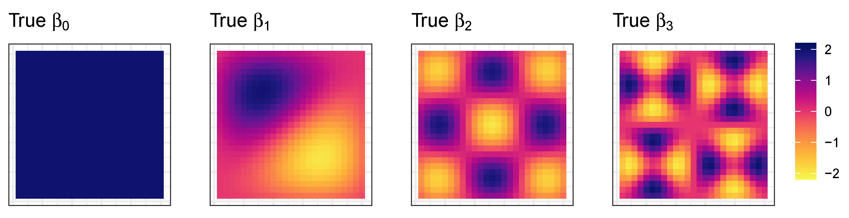
For the first analysis comparing the proposed GGP-GAM and MGWR SVC models, a simulated spatially varying coefficient dataset was created, with three coefficients each having different degrees of spatial heterogeneity. This was created by extracting Moran eigenvectors [13] generated using the spmoran R package v0.3.3 [34]. Here, the 1st, 10th and 25th surfaces were selected from the matrix of the first L eigenvectors for a 25 by 25 grid (625 observations). Each coefficient surface, (termed , and ), had a normal distribution and was rescaled to have a mean of 0 and standard deviation of 1. An intercept surface () with a constant value of 2 was also defined. These represent the true regression coefficients and are shown in Figure 1.
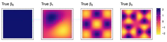
Figure 1.
Four simulated surfaces with varying degrees and forms of spatial heterogeneity that serve as the true spatially varying coefficients (n = 625).
One hundred simulated datasets were created from random generated values for , and with a specified normal distribution, a mean of 0 and a standard deviation of 1. Each of these was min–max-transformed to have a range of (0, 1). Values for the error term () were generated in a similar way but min–max-transformed to have a range of (0, 0.25). The simulated response (y) was calculated directly from these and the true coefficients (Figure 1).
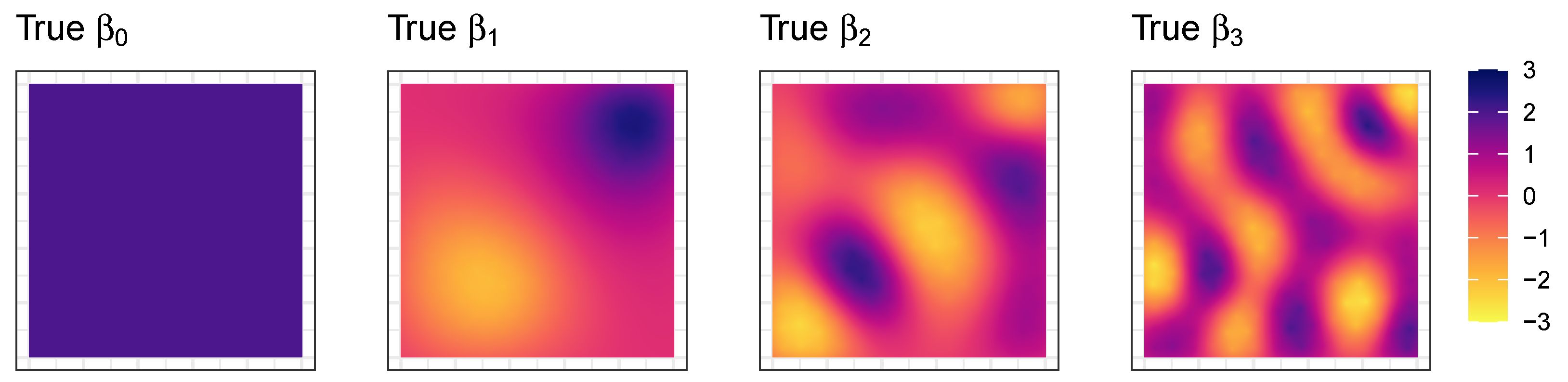
For the second analysis, a single simulated dataset was, again, created from Moran eigenvectors over a 500 by 500 grid. The 1st, 10th and 25th surfaces were extracted to create 250,000 observations with 3 true coefficients and an intercept surface with a constant value of 2. The coefficients had different spatial heterogeneities than those shown in Figure 1. Values for , , , and y were generated in the same way as for the smaller simulated study. The true coefficients are shown in Figure 2. Note that the range of the true coefficients is slightly larger than that of those in Figure 1, and their spatial variations are different.
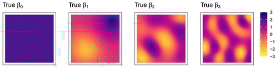
Figure 2.
True regression coefficient surfaces, with varying degrees of spatial heterogeneity, for a larger dataset (n = 250,000).
3.2. GAM-Based SVC Models
The standard form for an OLS regression is
where for observations indexed by , is the response variable, is the value of the j-th predictor variable, m is the number of predictor variables, is the intercept term, is the regression coefficient for the j-th predictor variable and is the random error term. This can be extended to define an SVC regression model:
where now are the spatial coordinates of the observations i and are the coefficients estimated at those locations.
GAMs can also calibrate regression models in which the functions of the predictor variables are unknown, taking the following form:
where is the intercept ( in Equations (1) and (2)) and the j-th predictor can be a scalar or a vector.
These can be extended so that each becomes a linear regression coefficient on another scalar predictor in a linear regression ():
Furthermore, if , for example, and z is a vector of locations or coordinates (similar to in Equations (1) and (2)), then a spatially varying coefficient model is specified:
where represents the j-th SVC.
One approach to specifying is to generate each function from a GP smooth defined as follows:
where represents a basis function, is the corresponding coefficient and is the smoothing parameter. SVC exhibits high spatial variation if is large and remains constant if . In this way, the smoothing parameter determines the wiggliness of the SVC, that is, how the function varies across its range.
The basis function () is specified such that has a spatially smooth pattern—in this case, driven by the following covariance function:
where represents the distance between locations z and and the covariance function decreases with increases in . This is similar to kriging and MGWR. Kriging uses covariance functions via the semi-variogram and a covariance function is calibrated individually for each in the same way as bandwidths are optimised in MGWR. Thus a key task in using GAMs to model SVCs is to estimate the smoothness parameters and thereby .
A GAM employs smooth functions of the predictor variables, assuming that the values of the response variable (y) follow some kind of exponential distribution:
where , , and are known functions and is a vector of parameters. This has a flexible form and is, thus, able to handle a wide range of distributions, including Gaussian, Poisson, gamma or binomial distributions.
In summary, GAMs can estimate SVCs by modelling non-linear relationships as spatially non-stationary distributions using GP splines parameterised over geographical and attribute space, and a GP spline with spatial location is defined for each predictor variable (j). Additionally, an offset () is added to account for the GP’s zero mean, thereby creating the SVCs (). In the standard 2D case, defines the geographical Gaussian process GAM (GGP-GAM).
3.3. Analysis I: Comparing GGP-GAM and MGWR
GAMs with GP were undertaken using the gam function in the mgcv R package [35]. The observed spatial locations (z) were extracted and used to parameterise the splines with a GP smooth. The GPs constructed in this manner had a mean of zero; therefore, an additional fixed offset term was included for each predictor variable alongside the spatially smoothed terms.
There are some important tuning considerations in fitting GAMs with mgcv, including the specification of spline smoothing parameters and the number of knots. These parameters influence the nature of the varying coefficients and the characterization of response-to-predictor relationships across space. The smoothing parameter regulates the degree of data smoothing through a correlation function, and the GAM function in the mgcv package optimises this using an estimation method. In this case, REML was specified for optimization instead of a cross-validation estimator. The number of knots (k) determines the basis dimensions; the maximum number of base functions used in the smooth; and, thus, the degree of sensitivity in fitting the model to the data. For example, consider the models predicting y specified with different numbers of knots in Figure 3. These determine the degree of relationship non-linearity in the smooth, together with the smoothing parameter. They are heuristically optimised by most GAM implementations in order to balance over-fitting with capturing relationship complexity. In the approach suggested by Wood [35], k can be manually and iteratively determined; an initial value is set, and the resultant splines are examined to determine whether the smoothing optimisation has converged and whether the basis dimensions defined by k are adequate. If not, they are increased. For the first analysis comparing GGP-GAM and MGWR, was specified after investigation.
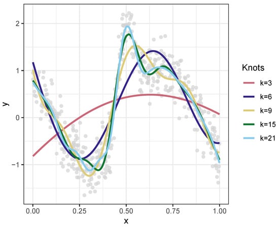
Figure 3.
The effect of increasing the knots specified in a GAM smooth on model accuracy.
The GWmodel R package [36,37] was used to construct the MGWR models, which were specified with an adaptive bisquare kernel. Note that fixed kernels were also investigated, and the comparisons with the GGP-GAM results reported below were found to be similar. MGWR accommodates and quantifies varying degrees of spatial heterogeneity in the predictor-to-response relationships by determining an optimal kernel bandwidth for each predictor variable. Implementations of MGWR use a back-fitting algorithm to do this [37,38,39]. Here, the convergence of the back-fitting procedure was evaluated through cross-validation of the residual sum of squares, and the threshold for convergence was set at or 2000 convergence iterations.
In the first analyses, the GGP-GAM and MGWR models were fitted to the 100 simulated datasets with 625 observations. The SVC estimates were extracted for each model, along with predictions of y (i.e., ) for each observation. Measures of fit were calculated from the model coefficient estimates with the true ones in Figure 1, including R2 for , and ( is stationary) and RMSE and MAE for , , and . Model AIC measures were also calculated. Finally, the model residuals () were also extracted to compare their spatial autocorrelation. To ensure consistency, functions for AIC, MAE, RMSE and R2 were coded rather than using the values generated by the outputs of the mgcv and the GWmodel packages.
3.4. Analysis II: GGP-GAM Tuning with a Larger Dataset
A second set of analyses investigated model tuning via the knots parameter (k) using a single larger dataset with 250,000 observations. The aim was to identify any trade-offs between performance, computational efficiency and accuracy. Seven GGP-GAMs were specified, each with an increasing number knots. The effects of increasing k were evaluated through computation time, coefficient accuracy and predictive performance. Again, these were implemented in the mgcv package but using the bam function with parallel processing. Each model had the same input data but with the k parameter varying.
3.5. Empirical Example: Brexit Vote
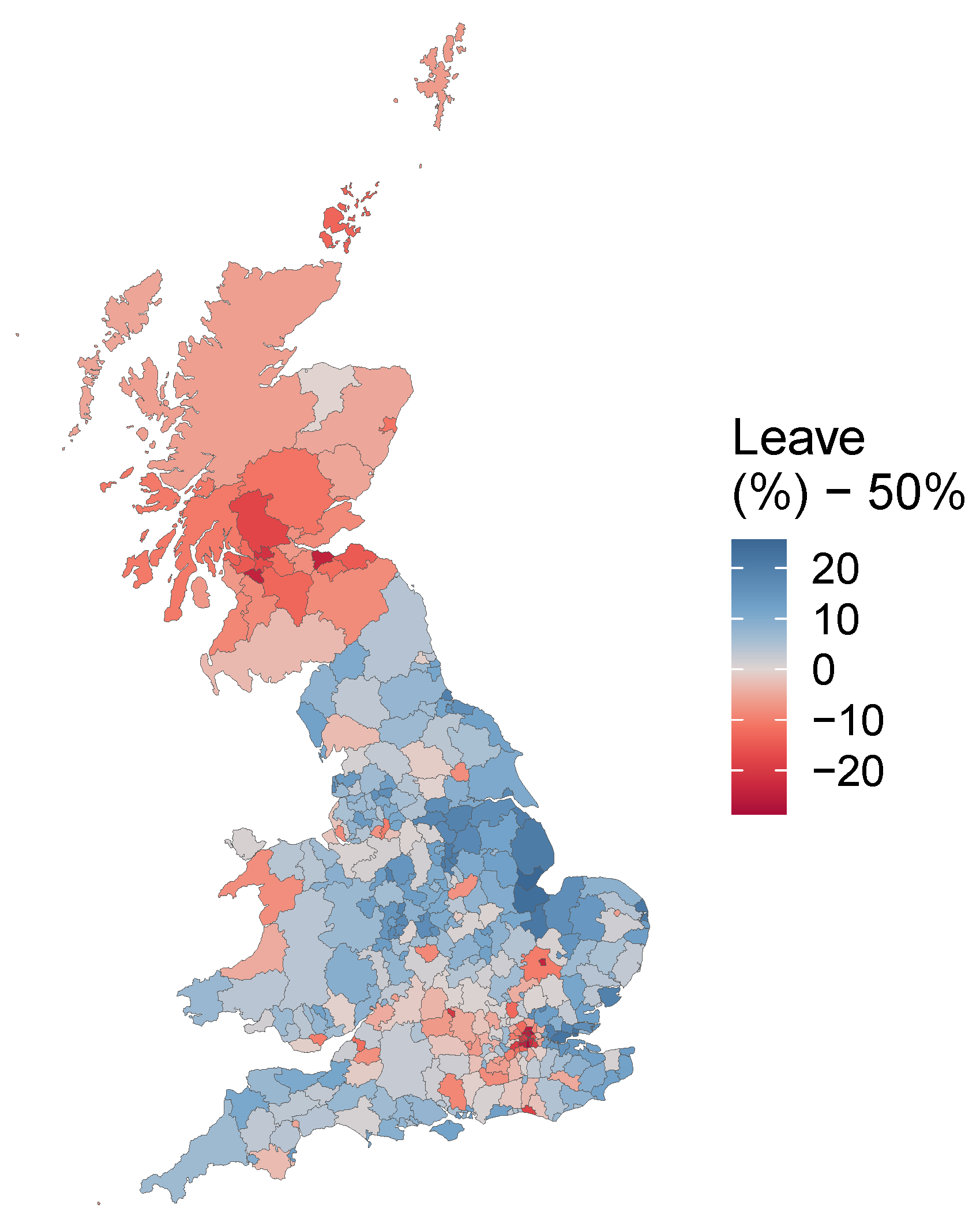
A final comparative analysis was undertaken using an empirical example. This used data from the 2016 referendum on leaving the European Union for England, Wales and Scotland (the Brexit vote) [40] and compared GGP-GAM and MGWR models. The spatial distribution of the Leave vote share (the response variable) over 380 Local Authority Districts is shown in Figure 4. This suggests that the overall outcome of a 51.9% majority in favour of ‘Leave’ conceals notable regional patterns. For this example, predictor variables from the 2011 UK Census were analysed: Christian is the proportion stating their religion as Christian, Degree is the proportion with a bachelor’s degree, No Car is the proportion who do not own a car or van and Younger is the proportion of the electorate between the ages of 20 and 44 years old. The variables were not rescaled.

Figure 4.
The ‘Leave’ vote share in the 2016 UK referendum on leaving the EU across Local Authority Districts (England, Wales and Scotland).
4. Results
4.1. Comparing GGP-GAM and MGWR
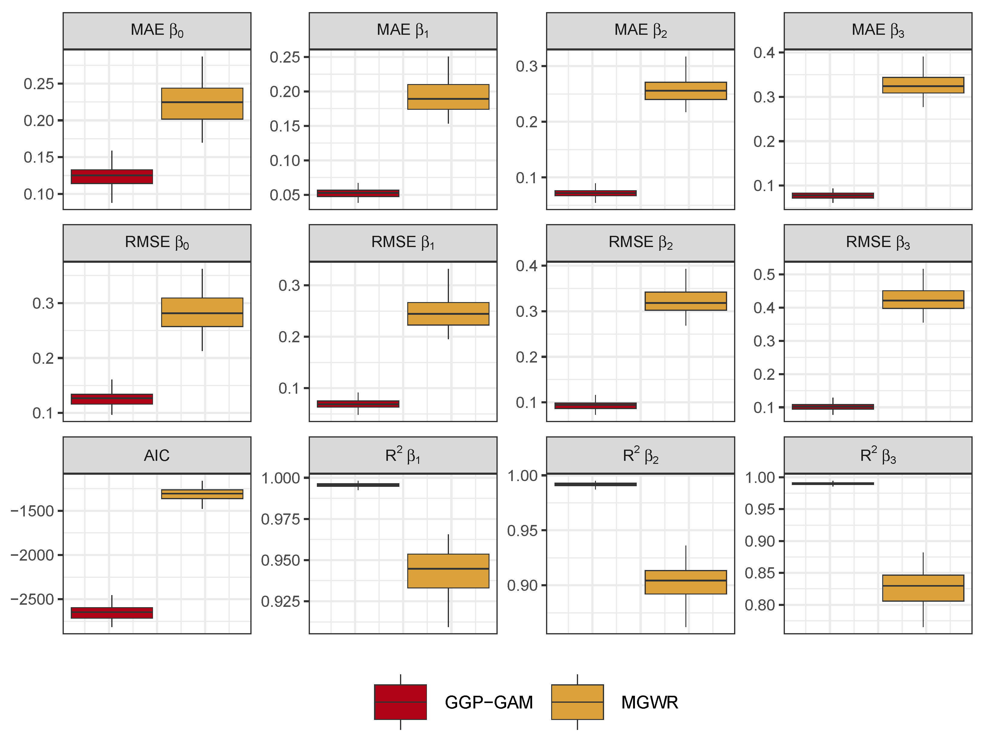
Evaluations of the estimated coefficients against the true coefficients arising from the 100 GGP-GAM and MGWR models are shown in Figure 5. The boxplots have the outliers removed to emphasise the differences between the median values in the fit measures. For each fit measure (RMSE, MAE and R2), the GGP-GAM provides more accurate estimates of the true coefficients than MGWR, with the difference increasing with the degree of spatial heterogeneity (i.e., from to ).
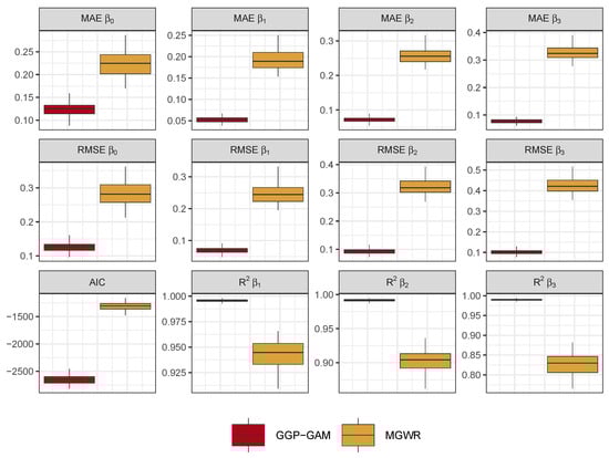
Figure 5.
Assessment of the accuracy of GGP-GAM and MGWR regression coefficient estimates when compared to the true coefficients, along with the distribution of model AIC values.
The distributions of model fit indicated by AIC show that the GGP-GAMs consistently have lower AIC values than the MGWR models. Investigations of these revealed them to be driven by differences in the residuals rather than the number of model parameters. These are summarised in Table 1.

Table 1.
Summaries of the residuals of the 100 GGP-GAM and MGWR models.
The spatial variation in the residuals was also compared. A Moran’s I statistic was generated for the residuals arising from each GGP-GAM and MGWR model. Their distributions are summarised in Table 2. The MGWR residuals have higher positive values, indicating stronger positive spatial autocorrelation (i.e., clustering), while the GGP-GAM residuals have more negative values, indicating stronger negative spatial autocorrelation (i.e., dispersion).
Table 2.
Summaries of the Moran’s I of the residuals of the 100 GGP-GAM and MGWR models.
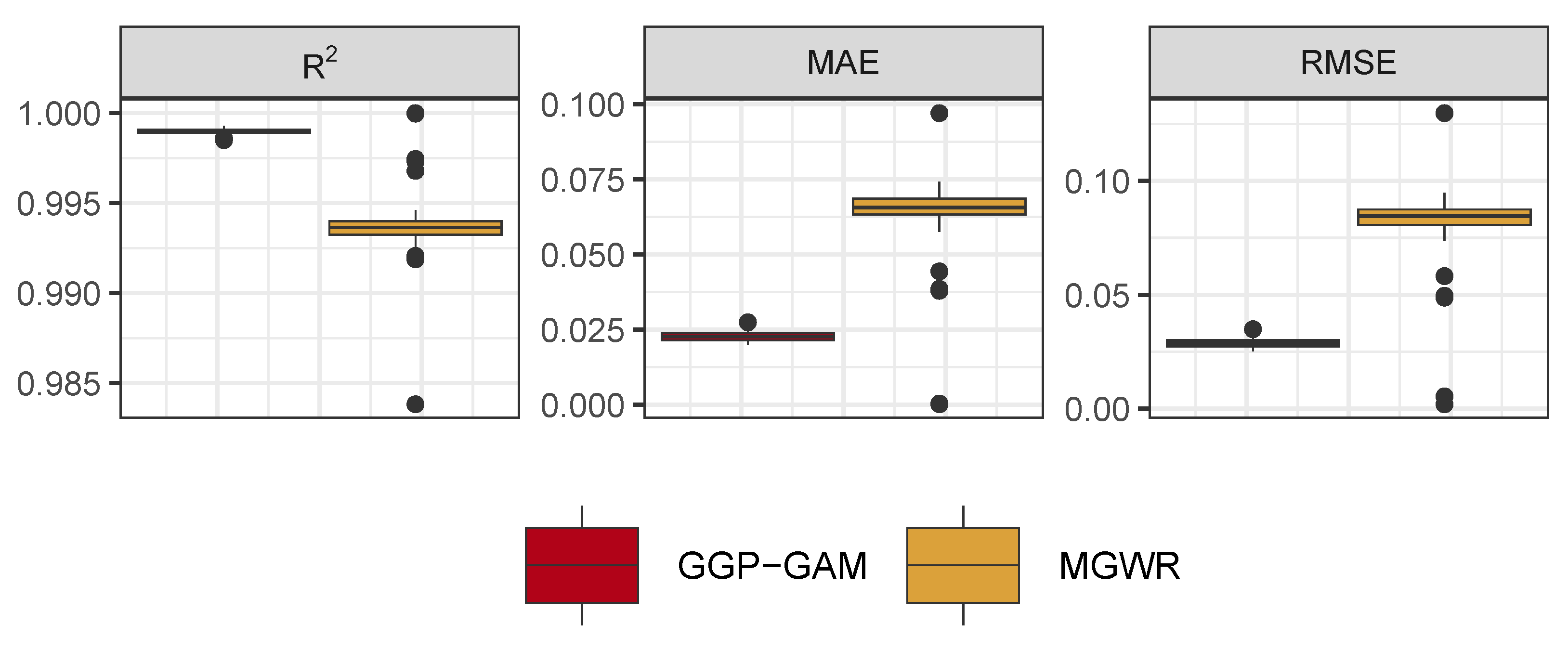
The accuracy of the predicted measures of y (i.e., ) arising from the two models are compared in Figure 6, using RMSE, MAE and R2. The GGP-GAMs generate more accurate predictions, reflecting their better of estimation of the true coefficients.

Figure 6.
The GGP-GAM and MGWR model fits.
Model calibrations were also investigated. The GGP-GAM spline smoothing parameters are part of a covariance function that penalizes model complexity, while the individual bandwidths in MGWR describe the scale of each predictor-to-response relationship and the scales of process spatial heterogeneity. These are summarised in Table 3. The homogeneity of these, as indicated by the inter-quartile ranges, reflect the convergence of the bandwidth optimisation in the MGWR models and the optimisation of the spline smoothing parameters in the GGP-GAMs.
Table 3.
The distributions of MGWR bandwidths (BW) and GGP-GAM spline smoothing parameters (SP).
4.2. A Single GGP-GAM in Detail
It is instructive to examine the nature of a GGP-GAM and its coefficients in detail. The 51st model was randomly selected, and its properties were examined. Diagnostics summaries of the model SVCs are shown in Table 4. These are generated by the gam.check function in the mgcv package. This summarises the results of the model optimisation procedures and allows the basis dimensions defined by k to be evaluated. Wood [24] noted that a “low p-value and a k-index of <1) may indicate that k is too low, especially if effective degrees of freedom (EDF) are close to k”. Similar results were found for other randomly selected models. It is evident that a k value of 155 is adequate: the EDFs are lower than k, and all the p-values are high.
Table 4.
Diagnostics of the GGP-GAM smoothing optimisation for the SVCs of a single GGP-GAM.
It is also possible to examine the fixed (parametric) coefficient estimates. These can be considered as the global model terms, similar to the outputs of a standard OLS regression, and are shown in Table 5. The effect of the large k is evident: the intercept has a significant global effect, and the fixed global relationships between the response and the predictor variables are reduced to zero.
Table 5.
The fixed (parametric) coefficients for a single GGP-GAM.
Table 6 summarises the smooth terms, the geographic GP splines. The full set of coefficients are not printed because there many coefficients for each spline—one for each basis function. The edf (effective degrees of freedom) indicates the spline complexity, with higher edf values suggesting increasing non-linearity in the predictor-to-response relationship. For example, an edf of 1 suggests a linear relationship, an edf of 2 indicates a quadratic relationship, etc. In this context, these values apply to each predictor variable across a two-dimensional space defined by , and the p-values indicate the significance of any spatial variation in the coefficient estimates, i.e., whether they vary significantly over space. In this case, the SVCs for , and are locally significant, but the intercept () is not.
Table 6.
The spline smooth terms for a single model.
It also is possible to examine whether and how the relationships between y and the predictor variables vary spatially, i.e., the SVCs. Table 7 summarises these for the single GGP-GAM. These reflect the relatively low spatial variation in the intercept and its globally significant effect, as well as the relatively high spatial variation in the coefficient estimates for , and .
Table 7.
Summaries of the spatially varying coefficients for a single GGP-GAM.
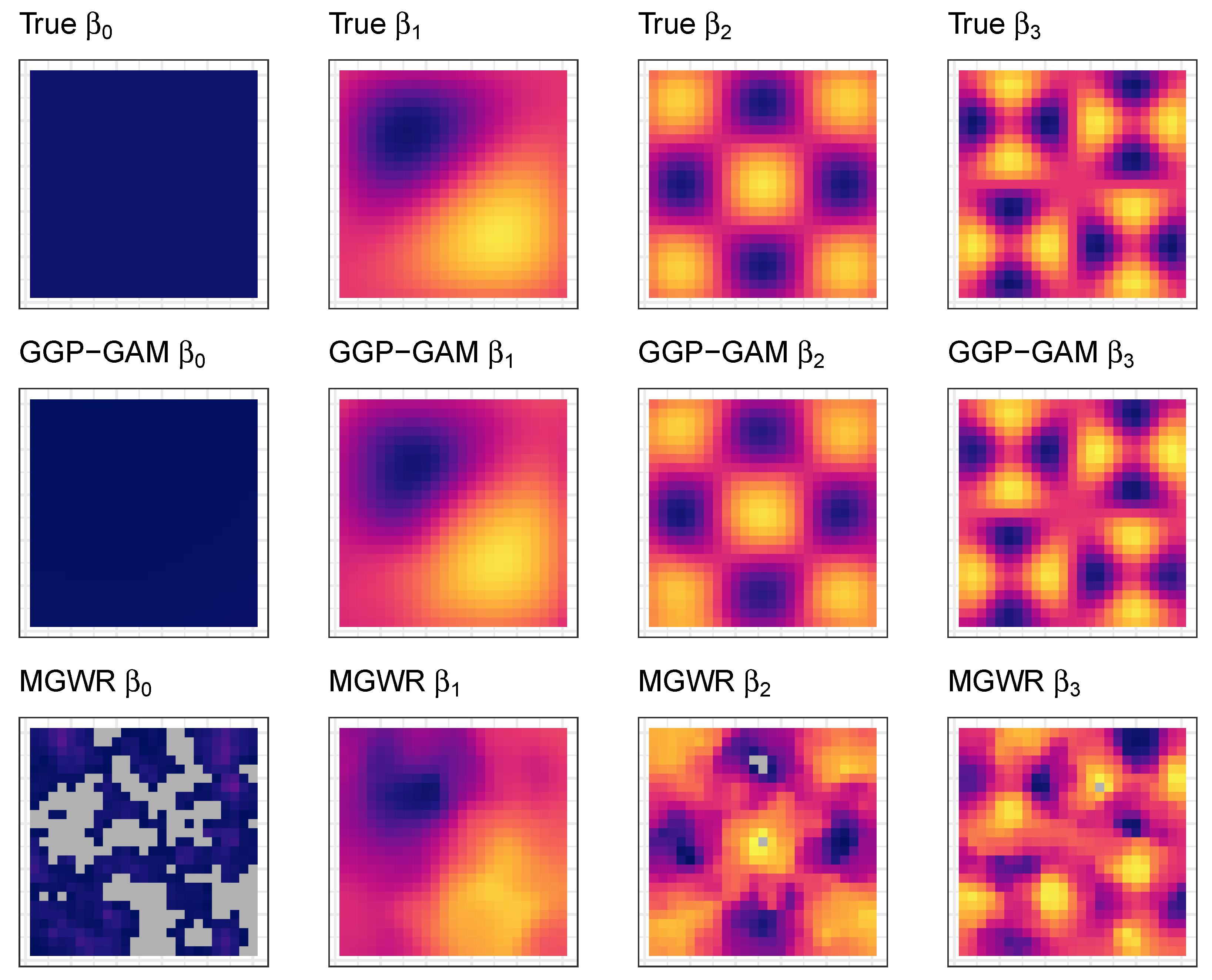
A final investigation mapped the GGP-GAM and MGWR SVCs alongside the true coefficients (Figure 7). The GGP-GAM and MGWR coefficient estimates are generated from the same input data, and the shading range was intentionally set to the same as Figure 1. The coefficient estimates for , , and indicate the better performance of the GAM-based approach over MGWR. The grey areas in the MGWR coefficient estimates indicate predicted values outside of the shading range.
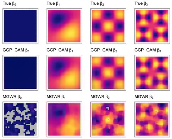
Figure 7.
The true coefficients with the GGP-GAM and MGWR estimated spatially varying coefficient surfaces modelled from a single simulated dataset.
4.3. GGP-GAM Tuning with a Larger Dataset
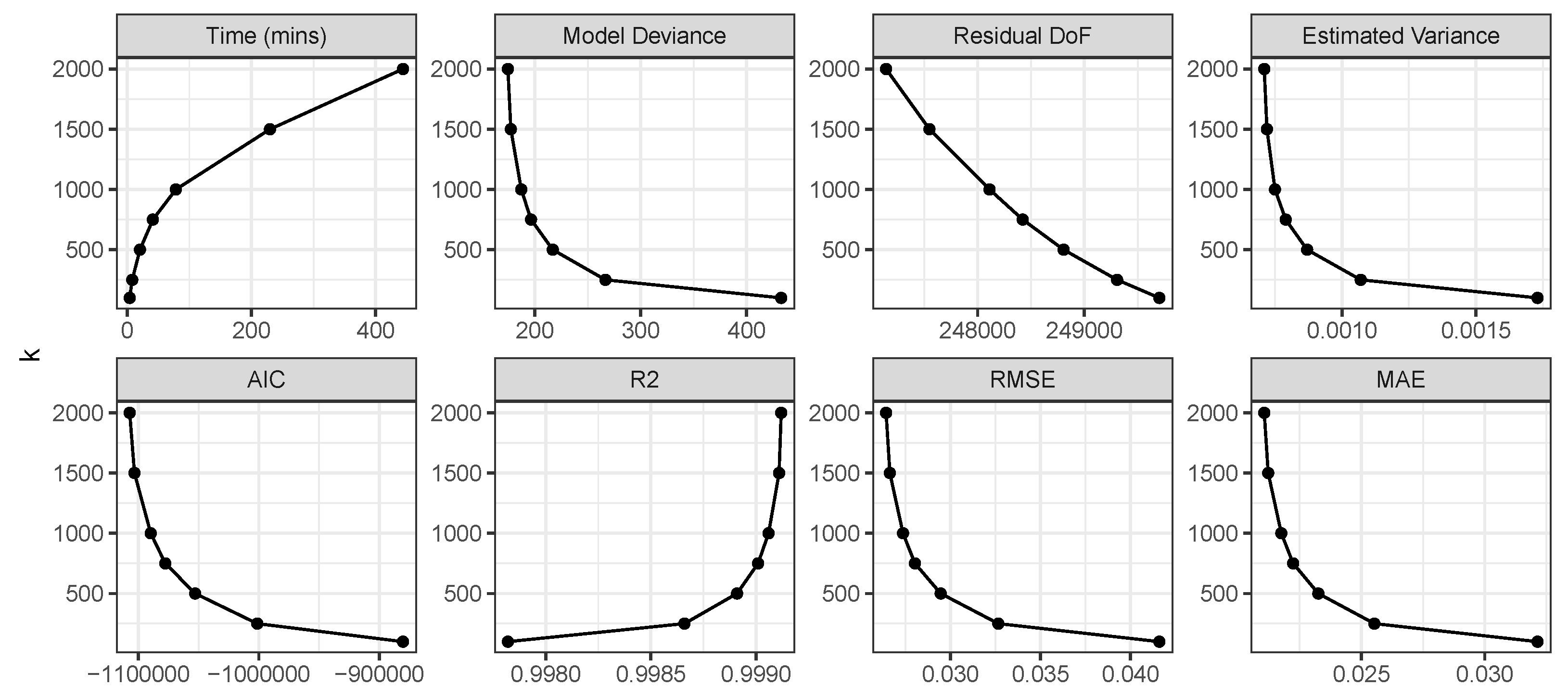
A second set of analyses investigated the impact of increased observation number and tuning via the knots parameter for 250,000 observations over a 500 by 500 grid (Figure 2). Seven GGP-GAMs were constructed but specified with different values of k: 100, 250, 500, 750, 1000, 1500 and 2000. Evaluations included computation time, coefficient accuracy and model-fit metrics. These are shown in Figure 8. Model deviance (unpenalized), the effective model residual degrees of freedom and the estimated variance parameter all decrease with increased k, as might be expected. The model fits also increase as the degree of tuning increases with higher values of k. There is a distinct elbow to many of these trends, suggesting suggests that a trade-off is possible between more complex but accurate models and increased computation times with higher values of k.
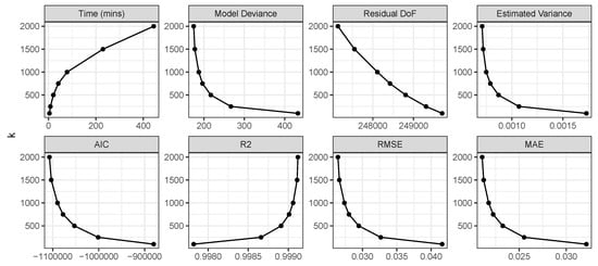
Figure 8.
The GGP-GAM metrics and fits with an increasing number of knots k.
Table 8 summarises the residuals arising from the different GGP-GAMs. They have similar central tendencies, and the inter-quartile ranges indicate that although the models with higher values of k have a lower variation, the differences are not dramatic. Again, this reinforces the possibility of a trade-off between model complexity and accuracy.
Table 8.
Summaries of the GGP-GAM residuals with increasing values of k.
The fixed parametric coefficient estimates of the seven models were investigated to examine the degree to which the effects observed in Table 5 for the small single GGP-GAM were also found (i.e., a significant intercept and insignificant predictor variables whose coefficients were zero). These are shown in Table 9. Whilst the intercept () has similar values and is always significant, the trends in the other predictor variables are more variable, especially at lower values of k. However, they are generally not significant when .
Table 9.
Summaries of the GGP-GAM fixed parametric coefficients with increasing values of k.
Table 10 summarises the geographic GP splines (the smooth terms) for the seven models. Recall that the effective degrees of freedom (edf) summarise the complexity of the spline smooths and the p-values indicate whether the coefficients are locally significant. In the model constructed for the single smaller dataset summarised in Table 6, the spatially varying intercept was not significant local, but all the other predictor variables were. The same pattern is found with the larger data, but notice how the effective degrees of freedom increase with k.
Table 10.
The effective degrees of freedom (edf) of the GGP spline smooth terms and their local significance (p-val) with increasing values of k.
The GGP-GAM spline smoothing parameters from the different models were examined. The homogeneity of these indicate the model convergence as determined by k, which defines the spline basis dimensions. These are summarised in Table 11. Two trends are evident in the smoothing parameter values across all values of k: the heterogeneity of the intercept across the different values of k, reflecting its global significance and local insignificance (Table 9 and Table 10), and the homogeneity within each predictor variable, with values of the same order of magnitude across different values of k.
Table 11.
The GGP spline smoothing parameters with increasing k values.
In summary, a series of GGP-GAMs was constructed using a larger simulated dataset with different values of k. As k increases, the number of spline bases increases and the models take longer to fit, indicating the trade-off between model complexity, accuracy and computation time. A distinct elbow was found with increasing k values in model deviance, residual degrees of freedom and estimated variance, as well as in the model-fit measures (AIC, R2, RMSE and MAE), suggesting possible trade-offs at around to (Figure 6). The residuals of these models were found to be similar to those of the models with high values of k (Table 8), where greater tuning might be expected to result in more accurate models. Except for the intercept, the global parametric coefficients flatten out or are insignificant at all values of k (Table 9), and all the predictor variables are locally significant at all values of k (Table 10), supporting trade-offs at values of k between 500 and 750 in this case.
4.4. Empirical Example: Brexit Vote
A final empirical analysis compared GGP-GAM and MGWR SVC models of the 2016 UK referendum on leaving the EU in England, Wales and Scotland (Figure 4). The model summaries are shown in Table 12, and in this case, both models perform well in terms of fit metrics (R2, AIC, MAE and RMSE), with the MGWR model marginally out-performing the GGP-GAM, although the GGP-GAM was computationally more efficient. However, perhaps of greater interest are the minor differences in coefficient estimates as summarised in Table 13 and Table 14 and mapped in Figure 9. The tables include the significance of the GGP-GAM smooth (i.e., the spline generating local coefficient estimates) and the MGWR bandwidths, whose sizes indicate the scale or degree of localness of each predictor-to-response relationship (their theoretical maximum is 1198 km).
Table 12.
Fit measures from the GGP-GAM and MGWR models of the Brexit vote.
Table 13.
Summaries of the SVCs for the Brexit GGP-GAM.
Table 14.
Summaries of the SVCs for the Brexit MGWR model.

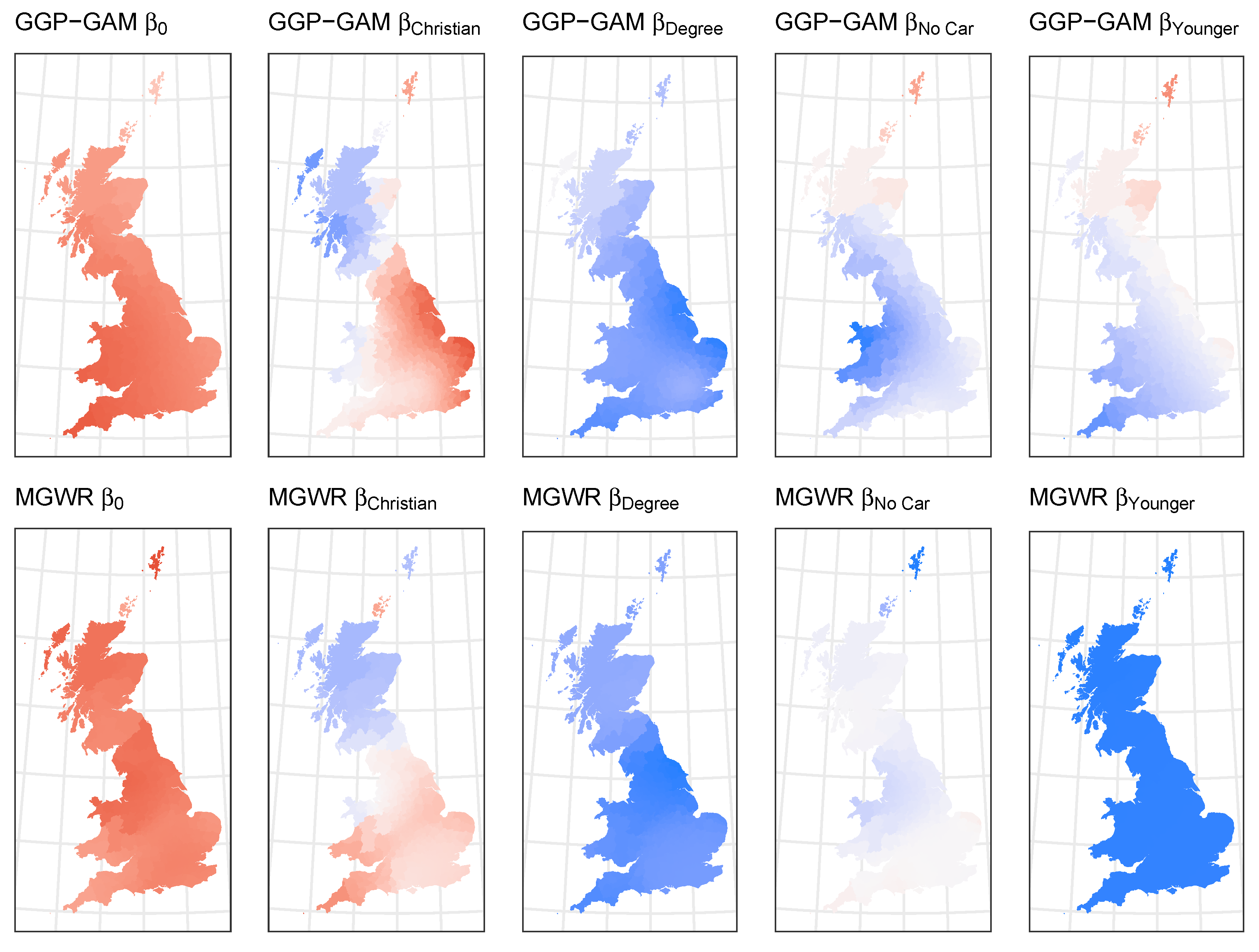
Figure 9.
The GGP-GAM and MGWR regression coefficient estimates, shaded using a diverging palette to indicate negative (blue) and positive (red) values.
Overall, when the central tendencies and inter-quartile ranges are examined, the two sets of coefficient estimates have similar values and ranges. Considering each in turn, a number of observations can be made:
- Intercept (): This is not locally significant in the GGP-GAM but is in its parametric form (not shown). The MGWR model indicates that it has a highly localised (i.e., spatially varying) relationship with a relatively small bandwidth. Both sets of coefficient estimates are positive and have similar values and ranges.
- Christian: Both sets of coefficient estimates indicate a negative association with the Leave vote in Scotland and parts of North Wales and a positive one in England. They are locally significant in the GGP-GAM and exhibit moderate local variation in the MGWR model, with a bandwidth of 159 km.
- Degree: This is locally significant in the GGP-GAM and is negatively associated with the Leave vote throughout the study area in both models. It indicates moderate local variation in the MGWR bandwidth (204 km).
- No Car: This is locally significant in the GGP-GAM. It is mostly negatively associated with the Leave vote share in both models and indicates similar areas of positive association with the Leave vote share in the north. The MGWR bandwidth indicates moderate local variation (172 km).
- Younger: This is not locally significant in the GGP-GAM, and in the MGWR its bandwidth is 1196 km. These both indicate that this predictor variable is globally (evenly) associated with the target variable.
In summary, the two models have similarly high fit and accuracy metrics and suggest subtly different process spatial heterogeneities and non-stationarities in the relationships between the target variable and the different predictor variables. These are more apparent in the extremes of the study area, potentially reflecting the mechanics of the moving window approach in GWR-based models.
5. Discussion
There is increasing interest in SVC models because of their ability to accommodate, capture and describe process spatial non-stationarity via regression coefficient estimates that vary geographically. Data are increasingly spatial (i.e., observation location is included in some form), and consequently, more researchers are working with spatial data. SVC models are attractive because they provide an indication of how and where statistical relationships vary over space, and the results can be mapped, providing insights about the spatial heterogeneity of the process being examined.
Some initial work has proposed SVC models using GAMs with Gaussian process smooths that include observation location—a Geographical GP GAM (GGP-GAM)—and a comparative study with MGWR was undertaken [33]. This used a different, less spatially complex set of simulated data to those presented here and accepted the default settings for GAMs in the mgcv package [35]. In this study, GGP-GAM and MGWR were applied to a more spatially complex set of simulated data (i.e., with much greater spatial heterogeneity), and the GGP-GAMs were tuned by specifying a sufficiently large number of knots such that the properties of the smooths converged. This was because the number of knots defines the basis dimension in the GP splines and the high value ensured sufficient degrees of freedom in each of the smooths. MGWR tuning was automatically undertaken during bandwidth optimisation.
The first part of this study compared GGP-GAM and MGWR SVC models of 100 simulated datasets, each with 625 observations. The GGP-GAMs performed better than MGWR across a range of fit measures, although a higher degree of variation was found in the GGP-GAM smoothing parameters than in the MGWR bandwidths (Table 3). The GGP-GAM generated more accurate coefficient estimates than MGWR, a finding that was confirmed when the MGWR analyses were re-run with fixed distance bandwidths rather than adaptive ones. On investigation, the difference in performance was found to be due to the relatively higher residuals arising from the MGWR models, although, objectively, both models performed well. This resulted in the MGWR model struggling to estimate the known, true coefficients (Figure 7) and suggests that MGWR models (and potentially other geographically weighted approaches) may struggle with more complex, highly localised spatial heterogeneities due to their rudimentary kernel/moving window-based formulation. Further investigation is required to confirm this assertion.
A second set of analyses applied the GGP-GAM to a larger simulated dataset, and a series of models were constructed with varying values of k, defining the number of knots. The results indicate excellent measures of fit at all values of k, and a degree stability in the GGP spline smooths was found for , suggesting that acceptable degrees of trade-off are possible between model complexity, computation times and GGP-GAM stability. Identifying the value of k at which model performance stabilises has operational benefits: the value of k determines the upper limit on the effective degrees of freedom linked to spline smoothness and, consequently, the spline bases. Increasing k also prolongs computation time. However, determining the optimal k algorithmically for a given case study is challenging. A common approach is to explore various k values and increasing and decreasing them as necessary. Here, it was shown that the gains at values of resulted in marginal performance gains at the cost of increases in computation time (a few minutes vs. a few hours).
The final analysis constructed and compared GGP-GAM and MGWR SVC models of the UK’s Brexit referendum vote to leave the European Union in 2016 with a small number of socio-economic variables. Both approaches generated similarly accurate models in terms of the ability to model the Leave vote share. The spatially varying coefficient estimates they generated indicated minor differences locally, with perhaps the greatest differences evident in the extremes of the study area. Consider, for example, the coefficients for Christian and No Car in the Shetland Islands in Figure 9: these are positive in the GGP-GAM and negative in the MGWR model, reflecting the smoothing effect of the GWR-based moving window approach and, potentially, the adaptive distance kernel. There were also difference in the predictor variables that were found to have a local relationship with the target variable. In sum, the MGWR and GGP-GAM approaches generated similar understandings of the process in this empirical case study but with differences in the geographical extremes. This may be due to the way that GWR-based approaches capture spatial non-stationarity: they move a weighted window across observations and estimate coefficients at each location rather than quantifying local variation in ‘data’ space [22]. Further work will seek to unpack these differences.
Other of areas of work are suggested by the findings of this study. One is to explore how the GGP-GAM approach may be further calibrated through out-of-sample predictions over randomly selected spatial data subsets. MGWR approaches are unable to do this because of their iterative back-fitting approach to model calibration. As a consequence, they cannot be applied to ‘new’ data. Another is to continue to extend the stgam R package [41]. Initial work on spatially varying coefficient modelling using GGP-GAMs simply coded the analysis in R. But as analyses progressed, the stgam package was developed to contain tools and wrapper functions for creating SVC models using GAMs with GP smooths. The functionality of this toolkit will continue to be expanded. One particular area of development is the generation of explicit measures of the scale of spatial dependencies in the coefficient estimates. In MGWR, this is provided by the kernel bandwidth, and in GGP-GAMs, a similar indication of scale could be to determine the variogram range for each spatially varying coefficient. There are also further opportunities arising from the core theory underpinning GAMs [7,8,35]. GGP-GAMs are more flexible than GWR-based approaches. They are inherently multiscale through their specification, and they are able to handle different responses, as well as having options for handling collinearity, outliers, and heteroskedastic and autocorrelated error terms—options that are not readily available for MGWR, aside from recent work on MGWR with autocorrelated errors [42] and Poisson responses [6]. Finally, extensions into space-time will be explored to investigate how to model space-time dependencies [43], potentially using model averaging [44] to determine optimal space-time model form. The ability to construct coefficient models in which the coefficients are allowed to vary over space and/or time is key in, for example, analysis of resilience to climate change, where the aim is to determine the varying drivers of changes in resilience and to predict tipping points.
6. Conclusions
This study describes spatially varying coefficient modelling using GAMs with Gaussian process splines parameterised with observation location, referred to as geographical Gaussian process GAM (GGP-GAM). In a series of analyses, GGP-GAM was applied to simulated data with known and complex spatial heterogeneities and found to perform better than MGWR, the SVC brand leader. This raises questions about the ability of kernel-based approaches like GWR to handle highly localised processes. GGP-GAM was then applied to a larger datasets to investigate model tuning. Processes for determining acceptable trade-offs between model complexity, computational efficiency and stability were identified with respect to the number of knots used in the GP smooths. Finally, the GGP-GAM and MGWR were applied to an empirical case study of the 2016 UK Brexit referendum vote. Both models performed well in terms of fit metrics, with the MGWR model marginally out-performing the GGP-GAM. The coefficient estimates generated by the two approaches for each predictor variable were broadly similar in terms of their sign (positive/negative), their mapped spatial distributions and the degree of local heterogeneity they suggested. However, differences were found in the geographical extremes, likely due to the mechanics and smoothing effect of the moving window approach in GWR-based models. Further research will continue to the develop the GGP-GAM approach, including the R package that was created in this work, [41], handling responses with non-Gaussian distributions, and will extend into the temporal domain to generate spatially and temporally varying coefficient models.
Author Contributions
Conceptualization, Alexis Comber, Paul Harris, Daisuke Murakami and Chris Brunsdon; methodology, Alexis Comber, Paul Harris, Daisuke Murakami and Chris Brunsdon; code, Alexis Comber; validation, Alexis Comber, Paul Harris, Daisuke Murakami, Tomoki Nakaya, Narumasa Tsutsumida, Takahiro Yoshida and Chris Brunsdon; formal analysis, Alexis Comber, Paul Harris, Daisuke Murakami and Chris Brunsdon; investigation, Alexis Comber, Paul Harris, Daisuke Murakami and Chris Brunsdon; writing—original draft preparation, Alexis Comber; writing—review and editing, Alexis Comber, Paul Harris, Daisuke Murakami, Tomoki Nakaya, Narumasa Tsutsumida, Takahiro Yoshida and Chris Brunsdon. All authors have read and agreed to the published version of the manuscript.
Funding
This work was supported by The Japan Society for the Promotion of Science BRIDGE fellowship No. 220305; initial ideas were developed under research supported by NERC (NE/S009124/1) and BBSRC (BB/X010961/1, BBS/E/RH/230004C, BBS/E/RH/23NB0008).
Institutional Review Board Statement
Not applicable.
Informed Consent Statement
Not applicable.
Data Availability Statement
The data and code used to undertake the full GGP-GAM and MGWR analyses and to generate the results presented in this paper can be found at https://figshare.com/s/2038debc91a82986c503 and at https://github.com/lexcomber/GGP-GAM-tune.
Conflicts of Interest
The authors declare no conflicts of interest. The funders had no role in the design of the study; in the collection, analyses or interpretation of data; in the writing of the manuscript; or in the decision to publish the results.
References
- Openshaw, S. Developing GIS-relevant zone-based spatial analysis methods. In Spatial Analysis: Modelling in a GIS Environment; Wiley: London, UK, 1996; pp. 55–73. [Google Scholar]
- Brunsdon, C.; Fotheringham, A.S.; Charlton, M.E. Geographically weighted regression: A method for exploring spatial nonstationarity. Geogr. Anal. 1996, 28, 281–298. [Google Scholar] [CrossRef]
- Yang, W. An Extension of Geographically Weighted Regression with Flexible Bandwidths. Ph.D. Thesis, University of St Andrews, St Andrews, Scotland, 2014. [Google Scholar]
- Fotheringham, A.S.; Yang, W.; Kang, W. Multiscale geographically weighted regression (MGWR). Ann. Am. Assoc. Geogr. 2017, 107, 1247–1265. [Google Scholar] [CrossRef]
- Comber, A.; Brunsdon, C.; Charlton, M.; Dong, G.; Harris, R.; Lu, B.; Lü, Y.; Murakami, D.; Nakaya, T.; Wang, Y.; et al. A route map for successful applications of geographically weighted regression. Geogr. Anal. 2023, 55, 155–178. [Google Scholar] [CrossRef]
- Sachdeva, M.; Fotheringham, A.S.; Li, Z.; Yu, H. On the local modeling of count data: Multiscale geographically weighted Poisson regression. Int. J. Geogr. Inf. Sci. 2023, 37, 2238–2261. [Google Scholar] [CrossRef]
- Hastie, T.; Tibshirani, R. Generalized Additive Models. Stat. Sci. 1986, 1, 297–310. [Google Scholar] [CrossRef]
- Hastie, T.; Tibshirani, R. Generalized Additive Models; Chapman and Hall/CRC Press: Boca Raton, FL, USA, 1990. [Google Scholar]
- Gelfand, A.E.; Kim, H.J.; Sirmans, C.; Banerjee, S. Spatial modeling with spatially varying coefficient processes. J. Am. Stat. Assoc. 2003, 98, 387–396. [Google Scholar] [CrossRef] [PubMed]
- Finley, A.O. Comparing spatially-varying coefficients models for analysis of ecological data with non-stationary and anisotropic residual dependence. Methods Ecol. Evol. 2011, 2, 143–154. [Google Scholar] [CrossRef]
- Kim, H.; Lee, J. Hierarchical spatially varying coefficient process model. Technometrics 2017, 59, 521–527. [Google Scholar] [CrossRef]
- Finley, A.O.; Banerjee, S. Bayesian spatially varying coefficient models in the spBayes R package. Environ. Model. Softw. 2020, 125, 104608. [Google Scholar] [CrossRef]
- Murakami, D.; Griffith, D.A. Random effects specifications in eigenvector spatial filtering: A simulation study. J. Geogr. Syst. 2015, 17, 311–331. [Google Scholar] [CrossRef]
- Murakami, D.; Griffith, D.A. Balancing Spatial and Non-Spatial Variation in Varying Coefficient Modeling: A Remedy for Spurious Correlation. Geogr. Anal. 2023, 55, 31–55. [Google Scholar] [CrossRef]
- Murakami, D.; Yoshida, T.; Seya, H.; Griffith, D.A.; Yamagata, Y. A Moran coefficient-based mixed effects approach to investigate spatially varying relationships. Spat. Stat. 2017, 19, 68–89. [Google Scholar] [CrossRef]
- Griffith, D.A. Spatial-filtering-based contributions to a critique of geographically weighted regression (GWR). Environ. Plan. A 2008, 40, 2751–2769. [Google Scholar] [CrossRef]
- Mu, J.; Wang, G.; Wang, L. Estimation and inference in spatially varying coefficient models. Environmetrics 2018, 29, e2485. [Google Scholar] [CrossRef]
- Dambon, J.A.; Sigrist, F.; Furrer, R. Maximum likelihood estimation of spatially varying coefficient models for large data with an application to real estate price prediction. Spat. Stat. 2021, 41, 100470. [Google Scholar] [CrossRef]
- Fan, Y.T.; Huang, H.C. Spatially varying coefficient models using reduced-rank thin-plate splines. Spat. Stat. 2022, 51, 100654. [Google Scholar] [CrossRef]
- Comber, A.; Brunsdon, C.; Charlton, C.; Harris, P.; Lu, B.; Malleson, N. gwverse: A template for a new generic Geographically Weighted R package. arXiv 2021, arXiv:2109.14542. [Google Scholar]
- Wolf, L.J.; Oshan, T.M.; Fotheringham, A.S. Single and multiscale models of process spatial heterogeneity. Geogr. Anal. 2018, 50, 223–246. [Google Scholar] [CrossRef]
- Bivand, R.S.; Pebesma, E.J.; Gómez-Rubio, V.; Pebesma, E.J. Applied Spatial Data Analysis with R; Springer: Berlin/Heidelberg, Germany, 2008; Volume 747248717. [Google Scholar]
- Fahrmeir, L.; Kneib, T.; Lang, S.; Marx, B.D. Regression models. In Regression; Springer: Berlin/Heidelberg, Germany, 2021; pp. 23–84. [Google Scholar]
- Wood, S.N. Generalized Additive Models: An Introduction with R; CRC Press: Boca Raton, FL, USA, 2017. [Google Scholar]
- Friedman, J.H. Greedy function approximation: A gradient boosting machine. Ann. Stat. 2001, 29, 1189–1232. [Google Scholar] [CrossRef]
- Zschech, P.; Weinzierl, S.; Hambauer, N.; Zilker, S.; Kraus, M. GAM (e) changer or not? An evaluation of interpretable machine learning models based on additive model constraints. arXiv 2022, arXiv:2204.09123. [Google Scholar]
- Stasinopoulos, D.M.; Rigby, R.A. Generalized additive models for location scale and shape (GAMLSS) in R. J. Stat. Softw. 2008, 23, 1–46. [Google Scholar]
- Stasinopoulos, M.D.; Rigby, R.A.; Heller, G.Z.; Voudouris, V.; De Bastiani, F. Flexible Regression and Smoothing: Using GAMLSS in R; CRC Press: Boca Raton, FL, USA, 2017. [Google Scholar]
- Umlauf, N.; Adler, D.; Kneib, T.; Lang, S.; Zeileis, A. Structured additive regression models: An R interface to BayesX. J. Stat. Softw. 2015, 63, 1–46. [Google Scholar] [CrossRef]
- Umlauf, N.; Klein, N.; Zeileis, A. BAMLSS: Bayesian additive models for location, scale, and shape (and beyond). J. Comput. Graph. Stat. 2018, 27, 612–627. [Google Scholar] [CrossRef]
- Tobler, W.R. A computer movie simulating urban growth in the Detroit region. Econ. Geogr. 1970, 46, 234–240. [Google Scholar] [CrossRef]
- Williams, C.K.; Rasmussen, C.E. Gaussian Processes for Machine Learning; MIT Press: Cambridge, MA, USA, 2006; Volume 2. [Google Scholar]
- Comber, A.; Harris, P.; Brunsdon, C. Multiscale spatially varying coefficient modelling using a Geographical Gaussian Process GAM. Int. J. Geogr. Inf. Sci. 2024, 38, 27–47. [Google Scholar] [CrossRef]
- Murakami, D. spmoran: An R package for Moran’s eigenvector-based spatial regression analysis. arXiv 2017, arXiv:1703.04467. [Google Scholar]
- Wood, S.; Wood, M.S. Package ‘mgcv’; R Package Version; R Foundation for Statistical Computing: Vienna, Austria, 2015; Volume 1, p. 729. [Google Scholar]
- Lu, B.; Harris, P.; Charlton, M.; Brunsdon, C. The GWmodel R package: Further topics for exploring spatial heterogeneity using geographically weighted models. Geo-Spat. Inf. Sci. 2014, 17, 85–101. [Google Scholar] [CrossRef]
- Gollini, I.; Lu, B.; Charlton, M.; Brunsdon, C.; Harris, P. GWmodel: An R Package for Exploring Spatial Heterogeneity Using Geographically Weighted Models. J. Stat. Softw. 2015, 63, 1–50. [Google Scholar] [CrossRef]
- Lu, B.; Hu, Y.; Yang, D.; Liu, Y.; Liao, L.; Yin, Z.; Xia, T.; Dong, Z.; Harris, P.; Brunsdon, C.; et al. GWmodelS: A software for geographically weighted models. SoftwareX 2023, 21, 101291. [Google Scholar] [CrossRef]
- Oshan, T.M.; Li, Z.; Kang, W.; Wolf, L.J.; Fotheringham, A.S. mgwr: A Python implementation of multiscale geographically weighted regression for investigating process spatial heterogeneity and scale. ISPRS Int. J. Geo-Inf. 2019, 8, 269. [Google Scholar] [CrossRef]
- Beecham, R.; Slingsby, A.; Brunsdon, C. Locally-varying explanations behind the United Kingdom’s vote to leave the European Union. J. Spat. Inf. Sci. 2018, 16, 117–136. [Google Scholar] [CrossRef]
- Comber, L.; Harris, P.; Brunsdon, C. stgam: Spatially and Temporally Varying Coefficient Models Using Generalized Additive Models; R Package VERSION 0.0.1.0; R Foundation for Statistical Computing: Vienna, Austria, 2024. [Google Scholar]
- Geniaux, G.; Martinetti, D. A new method for dealing simultaneously with spatial autocorrelation and spatial heterogeneity in regression models. Reg. Sci. Urban Econ. 2018, 72, 74–85. [Google Scholar] [CrossRef]
- Comber, A.; Harris, P.; Brunsdon, C. Multiscale Spatially and Temporally Varying Coefficient Modelling Using a Geographic and Temporal Gaussian Process GAM (GTGP-GAM)(Short Paper). In Proceedings of the 12th International Conference on Geographic Information Science (GIScience 2023), Leeds, UK, 12–15 September 2023; Schloss Dagstuhl-Leibniz-Zentrum für Informatik: Wadern, Germany, 2023. [Google Scholar]
- Brunsdon, C.; Harris, P.; Comber, A. Smarter Than Your Average Model-Bayesian Model Averaging as a Spatial Analysis Tool (Short Paper). In Proceedings of the 12th International Conference on Geographic Information Science (GIScience 2023), Leeds, UK, 12–15 September 2023; Schloss Dagstuhl–Leibniz-Zentrum für Informatik: Wadern, Germany, 2023; Volume 277, p. 17. [Google Scholar]

Disclaimer/Publisher’s Note: The statements, opinions and data contained in all publications are solely those of the individual author(s) and contributor(s) and not of MDPI and/or the editor(s). MDPI and/or the editor(s) disclaim responsibility for any injury to people or property resulting from any ideas, methods, instructions or products referred to in the content. |
© 2024 by the authors. Published by MDPI on behalf of the International Society for Photogrammetry and Remote Sensing. Licensee MDPI, Basel, Switzerland. This article is an open access article distributed under the terms and conditions of the Creative Commons Attribution (CC BY) license (https://creativecommons.org/licenses/by/4.0/).