Article

Explaining Theft Using Offenders’ Activity Space Inferred from Residents’ Mobile Phone Data

1
Center of Geo-Informatics for Public Security, School of Geography and Remote Sensing, Guangzhou University, Guangzhou 510006, China
2
Department of Geography and GIS, University of Cincinnati, Cincinnati, OH 45221, USA
*
Author to whom correspondence should be addressed.
ISPRS Int. J. Geo-Inf. 2024, 13(1), 8; https://doi.org/10.3390/ijgi13010008
Submission received: 12 November 2023 / Revised: 18 December 2023 / Accepted: 23 December 2023 / Published: 26 December 2023

Abstract

:
Both an offender’s home area and their daily activity area can impact the spatial distribution of crime. However, existing studies are generally limited to the influence of the offender’s home area and its immediate surrounding areas, while ignoring other activity spaces. Recent studies have reported that the routine activities of an offender are similar to those of the residents living in the same vicinity. Based on this finding, our study proposed a flow-based method to measure how offenders are distributed in space according to the spatial mobility of the residents. The study area consists of 2643 communities in ZG City in southeast China; resident flows between every two communities were calculated based on mobile phone data. Offenders’ activity locations were inferred from the mobility flows of residents living in the same community. The estimated count of offenders in each community included both the offenders living there and offenders visiting there. Negative binomial regression models were constructed to test the explanatory power of this estimated offender count. Results showed that the flow-based offender count outperformed the home-based offender count. It also outperformed a spatial-lagged count that considers offenders from the immediate neighboring communities. This approach improved the estimation of the spatial distribution of offenders, which is helpful for crime analysis and police practice.

1. Introduction

The routine activity theory explains that crime generally occurs because of the convergence of potential victims and potential offenders alongside a lack of supervision in specific geographic contexts [1]. Therefore, the accurate measurement of both victims and potential offenders’ routine activities is helpful in better explaining the spatio-temporal distribution of crime. There is a large amount of literature focusing on the measurement of potential victims and their impact on different types of crimes. From the early use of resident populations [2] to the use of physical facilities or points of interest that attract visitors [3] and further to the use of big data to represent ambient populations [4], research on potential victims has been increasingly refined in space and time.
Compared to research on victims, the measurement of potential offenders’ spatial distribution is limited to arrest data that provide the information on where they live and where they commit crimes. However, offenders’ routine activity spaces are not only limited to their residence and their crime scene, but also include the areas that they frequently visited. As Brantingham and Brantingham [5] stated, offenders commit crime in their activity spaces. Therefore, the measurement of offender activity spaces can help improve interpretations of the spatial distribution of crime. In practice, if the police were knowledgeable concerning offenders’ routine activities, then the efficiency of crime prevention and control, such as hot spot policing and targeted patrol, could be greatly improved [6].
To address the problem of incomplete measurement of the offenders, we proposed a flow-based method to estimate how offenders move in space. By calculating the flow matrix of residents in a community to other communities, the potential daily activity space of the offenders living in the same area could be inferred. With this approach, each community has an estimated count of offenders that includes both the offenders living there and offenders visiting there. Negative binomial regression models were constructed to test the explanatory power of this flow-based offender count in comparison with the home-based count and the spatial-lagged count that considers offenders from the immediate neighboring communities. Next, we will review routine activities, activity nodes, and mobility patterns to describe the theoretical background of the flow-based method.

1.1. Routine Activities and Activity Nodes

Crime tends to be spatially clustered. The crime-prone spaces overlap offenders’ daily activity spaces. For example, the areas where the burglars, robbers, or thieves once lived, the residence of their siblings and other places they may have visited, and places with low housing prices are often their targeted areas [7,8,9]. Activity nodes such as bus stops, bars, and Internet cafes are also hot spots with high crime rates as robbers frequently visit or pass by [10]. Brantingham and Brantingham [3] further divided these activity nodes into two categories: crime attractors and crime generators. Crime attractors are places that offer opportunities to attract motivated offenders. Crime generators are places that attract large crowds, who in turn draw offenders. Typical crime attractors and generators include but are not limited to barbers, fast-food restaurants, grocery stores [10], shopping and entertainment areas, subway stations, and high schools [11]. The literature in the Chinese context shows that crime attractors have no significant difference from crime generators, and crime attractors and generators are not separately treated in the models [12,13,14,15].
Further, studies found that not only activities nodes themselves, but also their surrounding areas would suffer higher crime risk than other areas. Bernasco, Block et al. [16] used a spatial-lagged model to examine the relationship between crime and robbers’ potential activity nodes with the spatial-lagged effect. It revealed that census tracts close to these activity nodes would also suffer more crimes than others. This was because offenders’ daily activities obey distance decay patterns from the activity nodes.
Most of the studies on the activity nodes of offenders are limited to the home location of the offenders. Recently, scholars have attempted to reveal more detailed daily activities of offenders. For example, Menting, Lammers [7] collected the major activity spaces reported by 78 offenders relating to 140 offences such as theft, burglary, vandalism, and robbery through an online self-survey in 2017. The detailed activity spaces could better explain offenders’ crime location choice strategy than residential areas alone. Further, it was found that the more frequently visited areas were more likely to be targeted by offenders.
However, such questionnaire approaches may lead to incomplete and inaccurate results due to limitations in the memory of offenders and their reluctance to provide complete and truthful responses. The advancement in electronic collection of trajectory data presents new opportunities. For example, Rossmo, Lu [17] used a GPS tracking method to record the paths taken by 16 parolees in relation to violent and drug offenses during the 8 days prior to the crime being committed and discovered that the offense locations were part of the activity areas the offender frequented before committing the crime. Griffiths, Johnson [18] applied mobile phone data records to analyze four British terrorists in the months before their attacks. Results showed that the attack scenes were close to the terrorists’ main activity nodes, such as their homes or other safe locations.
The aforementioned studies showed that offenders’ routine activities can be partially depicted by mobility or trajectory data collected from both questionnaires and electronic technology. However, due to the cost and other difficulties, only a few offenders’ routine activities were included in these studies. These small sample analyses may not be representative of all offenders, and more robust approaches are needed.

1.2. Mobility Patterns

The literature shows that the mobility patterns of offenders are similar to those of the general population, which is typically measured in three aspects: activity nodes, travel distance, and mobility flows. In terms of activity nodes, the general population spend most of their time in residential areas and workplaces [19,20,21]. In addition, supermarkets, bus stops, and other facilities serve as important anchor points for their daily routines [22]. These locations can also be crime attractors and crime generators [10,23,24].
Regarding distance, both residents’ and offenders’ routine travels obey distance decay patterns. The longer the distance, the less frequent the travel is. Several studies have documented such patterns [19,25,26] (Zhou et al. 2015, Shao et al. 2022, Sun and Dan 2015). The average morning peak and evening peak commuting distances in Haikou are 6.05 km and 5.83 km, respectively [26]. The average commuting distance of Shanghai residents is 8.88 km [25]. The same pattern holds for offenders [12,24,27]. On average, residential burglars in ZG City travelled 7.14 km [12], and thieves travelled 5.69 km to commit crimes [24]. Similarly, in Western countries, the average journey-to-crime distance is about 4 km in Sheffield, England [28], about 3.5 km in the town of Harrow, London [28], and 2 km in Ottawa [28,29].
A few studies compared the travels and flow patterns of residents and offenders. Bernasco studied 843 adolescents in the Netherlands and found that the adolescents with offender behavior visited slightly more places than those without offender behavior, but the radius and predictability of their activities were similar [13]. Their offenses included theft, burglary, assault, robbery, drug dealing, and public order offences. Song et al. suggested that the mobility flows of the thieves are consistent with the residents in ZG City [30]. Specifically, offenders’ crime location choice preferences were similar to residents’ home-to-work commuting preferences.
To sum up, criminology theories stipulate that the routine activities of offenders have a great influence on crimes; however, there is a lack of viable measurement of all the possible routine activities of offenders for large areas. Based on the recent findings that offenders’ mobilities, especially those of thieves and other property offenders, are similar to residents’ routine activities [15,30], this research selected theft as the crime type. It proposes a flow-based method to measure the routine activity space of offenders and tests the effectiveness of this measurement by comparing it against the home-based offender count and the spatial-lagged offender count.

2. Materials and Methods

This study chose ZG City as an example to estimate flow-based offender counts and their relationship with crime. ZG City is one of the most important metropolises in China. A relatively large number of crimes and arrestees offer the needed data for this study. Due to the confidentiality agreement, the city was named ZG City instead of its real name. Other studies followed the same practice, as crime data in China are not publicly available [31,32,33,34]. The unit of analysis is communities, or Shequ in Chinese. ZG City is divided into 2643 communities, the average area of the communities is 2.74 km2.

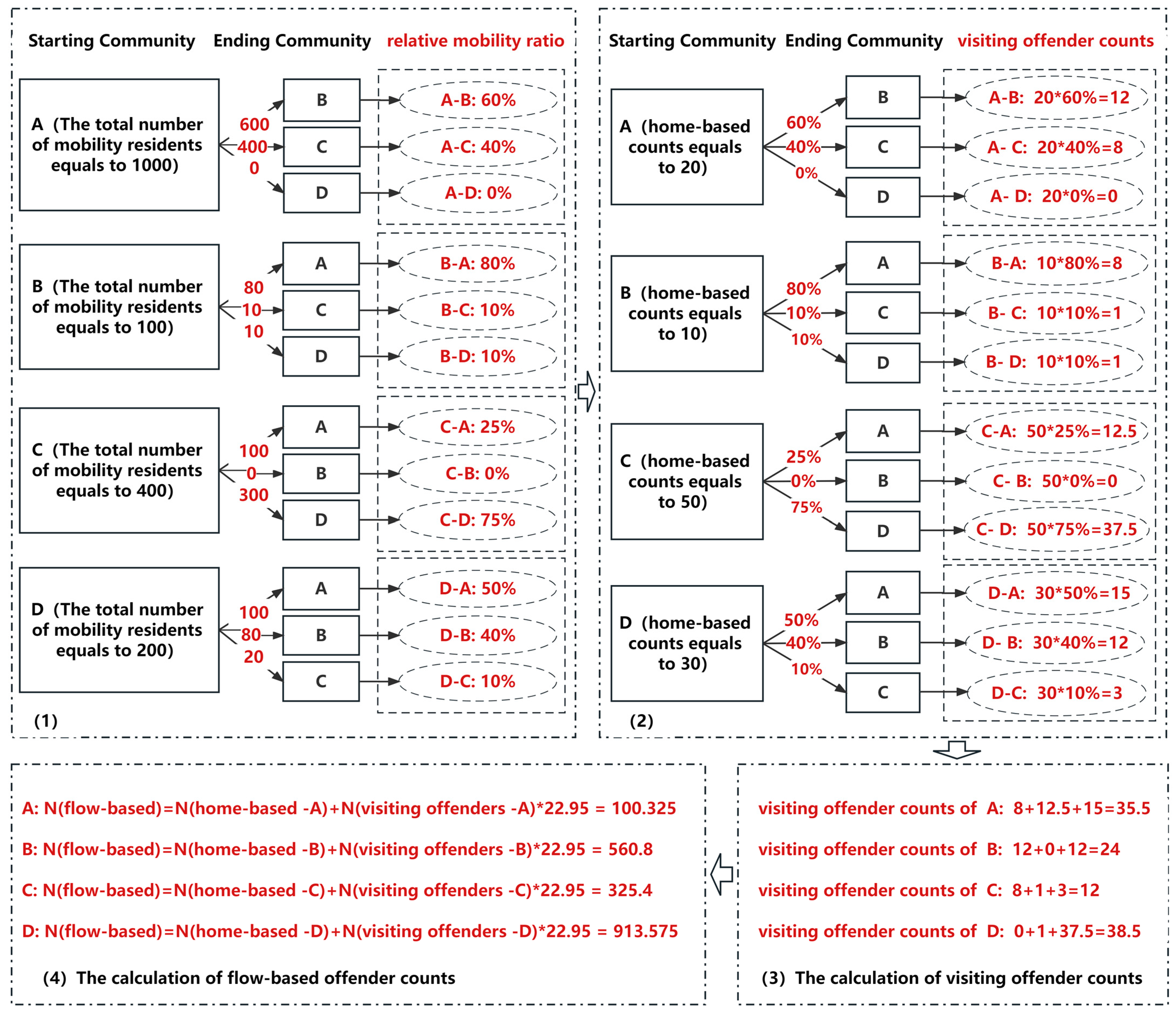
2.1. Estimation of Offender Counts (Independent Variables)

People’s mobility data comes from DAAS platform of Unicom, one of the three largest mobile phone service providers. The platform records the users who stay at a base station for more than 30 min. There was a total of 468 million travel records generated in October 2020 in ZG City. After desensitization and summarization of the data, this research extracts residents’ trajectory data, as shown below.
As shown in Table 1, each community has its unique 12-digit code. If a user had a trajectory from community A to B to C to D, it would be summarized as three trips: A to B, B to C, and C to D. A, B, and C are starting communities (O_Code), while B, C, and D are ending communities (D_Code). O_Ptype and D_Ptype represent a location classification of the starting community and ending community. A value of “0” means visiting community, “1” means home community, and “2” signifies the working community of the user. “Count” is the number of trips from the starting community to the ending community. In the first line of Table 1, community “440113105202” is the users’ home community, and community “440106011029” is the user’s work community. The number of trips made by the user from home to work is 2. This study only analyzed the flows that originated from home (O_Ptype = 1).
The data above contain the mobility flows of both residents and offenders. It is impossible to separate offenders from regular people. Offenders’ home locations were obtained from an arrestee database. The flow pattern of the offenders is assumed to be similar to those of the residents living in the same community. Thus, combined with both residents’ mobility and offenders’ residences, the flow-based offender counts of a community could be estimated as follows (see Figure 1):
Assuming that there are 4 communities labeled A, B, C, and D, and taking community A as an example, if 1000 trips originated from community A, with 600 trips destined to community B and 400 to community C, then the relative mobility ratio is 60% from community A to B and 40% from community A to C. Also, assuming that 20 offenders were known to live in community A, and that the offenders follow the above mobility ratios, the number of offenders would be 12 (20 × 60%) from community A to B and 8 (20 × 40%) from A to C. For each of the starting communities, replicate the above process to calculate the number of visiting offenders to each respective ending community. Finally, the visiting offenders to each community are summarized from all starting communities (Figure 1).
To test the effectiveness of the flow-based offender count, we compared it to two conventional counts of offenders. One is the home-based count of arrested offenders in each community. Among 2643 communities, 1117 communities had arrestees. The other is called the spatial-lagged count, which considers that offenders may also come from the immediate neighboring communities. Among the 3921 arrested offenders in ZG, 1191 offenders, or roughly 30% of all offenders, travelled less than 1.66 km to commit crime. Since the average size of communities is 2.74 km2, the average distance between the neighboring communities is roughly the square root of 2.74, which happens to be 1.66 km. Based on these two distances, it is reasonable to assume that 30% of the offenders may commit crime in the neighboring communities. Therefore, the spatial-lagged count is an addition of the home-based count and 30% of the home-based counts from the neighboring communities.
To make the flow-based count comparable to the spatial-lagged count, the summation of flow-based counts contributed from the neighboring communities is multiplied by a coefficient of 22.95 such that it is the same as the summation of spatial-lagged counts. The value of 22.95 is empirically calculated, and it may vary from one study area to another. The number of flow-based offenders for each focal community is calculated as follows:
N _ flow _ based j = N _ home _ based j + i = 1 i = 2643 N _ visiting ij × 22.95 ,   i , j = 1 , 2 , , 2643
where N _ flow _ based j is the flow-based offender count in community j. N _ home _ based j is the number of offenders living in community j. N _ visiting ij is the number of offenders visiting community j from community i where they live. The multiplier of 22.95 makes the flow-based count comparable to the spatial-lagged count. The calculation process is shown in Figure 1.

2.2. Dependent Variables and Covariates

The dependent variable in this study is the number of thefts in each community in 2018, which is provided by the Municipal Public Security Bureau of ZG City. For each community, the number of thefts can be counted using the intersection of community boundaries. The calculations were performed using the “sf” package in R.
Covariates include points of interest and the proportion of the migrant population. The point of interest data: Based on the routine activity theory, important activity places include the facilities that attract potential victims or potential offenders. Following prior studies [10,23,35,36,37], we chose bus stops, subway stations, Internet bars, KTVs, and cinemas as the important activity nodes in this study.
Proportion of the migrant population: The household registration system in China, known as the Hukou system, divides the population in a city into locals with a local Hukou and the migrant population (also known as nonlocals) with a Hukou registered in other cities. In Chinese metropolises, local Hukou groups typically include those who were born in the city or have transformed their outside Hukou to the city through higher education, permanent employment, or housing property ownership. In contrast, migrant populations typically do not have permanent employment, and cannot therefore transform their Hukou to the city. Although the Hukou system is not inherently based on socio-economic status, migrants typically have lower educational attainment and less income compared to the local Hukou group. Most migrants live in urban–rural transitional areas, villages in the city, and factory dormitories [27]. Previous studies have found that in Chinese cities, the proportion of the migrant population is an important factor for explaining crime [24,38]. Areas with a higher migrant population rate are commonly accompanied by more crimes [24,38]. Thus, following prior studies, the proportion of the migrant population was included in the analysis.

2.3. Regression Models

Three models were implemented using the home-based count, spatial-lagged count, and flow-based count. All models used the same dependent variable and control variables (or covariates).
Poisson regression models or negative binomial regression models are commonly used to model counts, such as the number of thefts in this study. Poisson regression models assume that the mean and variance of the dependent variable are equal [39]. The probability distribution function of a Poisson regression model is as follows:
P Y i = y i | X = e λ i λ i y i y i ! , i = 1 , 2 , 3 , 4
where P Y i = y i | X indicates the probability when the number of thefts Y i is y i and the explanatory variables Xs of community i are known. λ i is the number of thefts in community I and depends on a series of explanatory variables Xs. Furthermore, the conditional expectation function for Y i is commonly assumed as follows:
E Y i | X = λ i = e β X i
Var Y i | X i , β = λ i + α λ i
where α is the overdispersion parameter. If α equals to 0, the Poisson regression model should be used. When α is significantly greater than 0, the negative binomial regression model should be applied.
After logarithmic transformation of Equation (3), we obtain Equation (5) as follows:
ln λ i = β X i
However, crime counts are overdispersed, and Poisson regression models lead to underestimation of the standard error of coefficients [40]. The negative binomial regression model solves the problem of modeling overdispersed data by adding a residual term to the Poisson regression model in its log-transformed conditional expectation function, as shown in Equation (5). The newly constructed function is shown as follows:
ln λ i = β X i +   ε i
where the random variable ε i represents the unobservable part or the heterogeneity of individuals in the conditional expectation function. The residual is assumed to follow the gamma distribution, which reduces the miscalculation of the coefficient of explanatory variables and greatly improves the fitting degree of overdispersed data [14,41,42].
After considering the relationship between explanatory variables and the dependent variable, the following three models were finally constructed:
Model   1 :   ln λ i = β 0 + β N _ home _ based X N _ home _ based + β covariates X covariates +   ε i
Model   2 :   ln λ i = β 0 + β N _ spatial lagged _ based X N _ spatial lagged _ based + β covariates X covariates +   ε i
Model   3 :   ln λ i = β 0 + β N _ flow _ based X N _ flow _ based + β covariates X covariates +   ε i
In Model 1 to 3, in terms of dependent variables, λi is the number of thefts. In terms of independent variables, X N _ home _ based , X N _ spatial lagged _ based , and X N _ flow _ based are home-based offender count, spatial-lagged count, and flow-based offender count, respectively. X covariates includes bus stops, subway stations, Internet bars, KTVs, cinemas, and the proportion of the migrant population. In terms of coefficients, β 0 is the constant term, and β N _ home _ based , β N _ spatial lagged _ based , β N _ flow _ based , and β covariates are the coefficients for the independent variables accordingly. The coefficients were estimated with the maximum likelihood method.
Both unstandardized and standardized models can be useful. Unstandardized models use original independent variables to build models and directly display the quantitative relationship between independent variables and the dependent variable based on unstandardized coefficients. Different from unstandardized models, standardized models use independent variables that are standardized respectively to construct models. The standardized treatment makes the different independent variables have the same analysis scale in the same model. In each standardized model, it could compare the importance of the independent variables based on the standardized coefficients.
Since we need to verify which method of estimating the number of offenders can better explain crime, Akaike Information Criterion (AIC) and Bayesian Information Criterion (BIC) were used in this study [43,44]. Models with lower AIC and BIC usually have a better goodness-of-fit.

3. Results

3.1. Descriptive Statistics of Variables

Table 2 shows the descriptive statistics of the dependent and independent variables of a total of 2643 communities. As for the dependent variable, the average value of the number of thefts is 36.392. However, the maximum number of thefts in communities is 956, while there are also 153 communities with no cases. The variance of the dependent variable (61.110) is much larger than its mean value, indicating that the crime data are overdispersed.
In terms of the number of offenders estimated, the average values of the home-based offender count, spatial-lagged offender count, and flow-based offender count are 1.484, 3.677, and 35.348, respectively, indicating that offender count estimated by the flow-based method is higher than the other two methods. Additionally, the coefficient of variation is the highest in home-based offender count (1.353).
In terms of the covariates, there are more bus stops and Internet bars than other POIs in the communities. A community has an average of 2.544 bus stops, with a maximum of 102 bus stops. The average number of Internet bars is 1.102. The mean values for subway stations, KTVs, and cinemas are less than 1, but their coefficients of variation are much higher than those of bus stops and Internet bars. The average proportion of the migrant population is 27%, with a minimum of 0% and a maximum 97.4%.
All independent variables are significant and positively correlate to the number of thefts (Table 3). The flow-based offender count has the strongest correlation with crime, followed by the spatial-lagged offender count and home-based offender count. Internet bars and KTVs have the strongest correlation (0.506). A correlation coefficient less than 0.6 indicates that no serious multicollinearity problem exists in the model estimations [45,46].

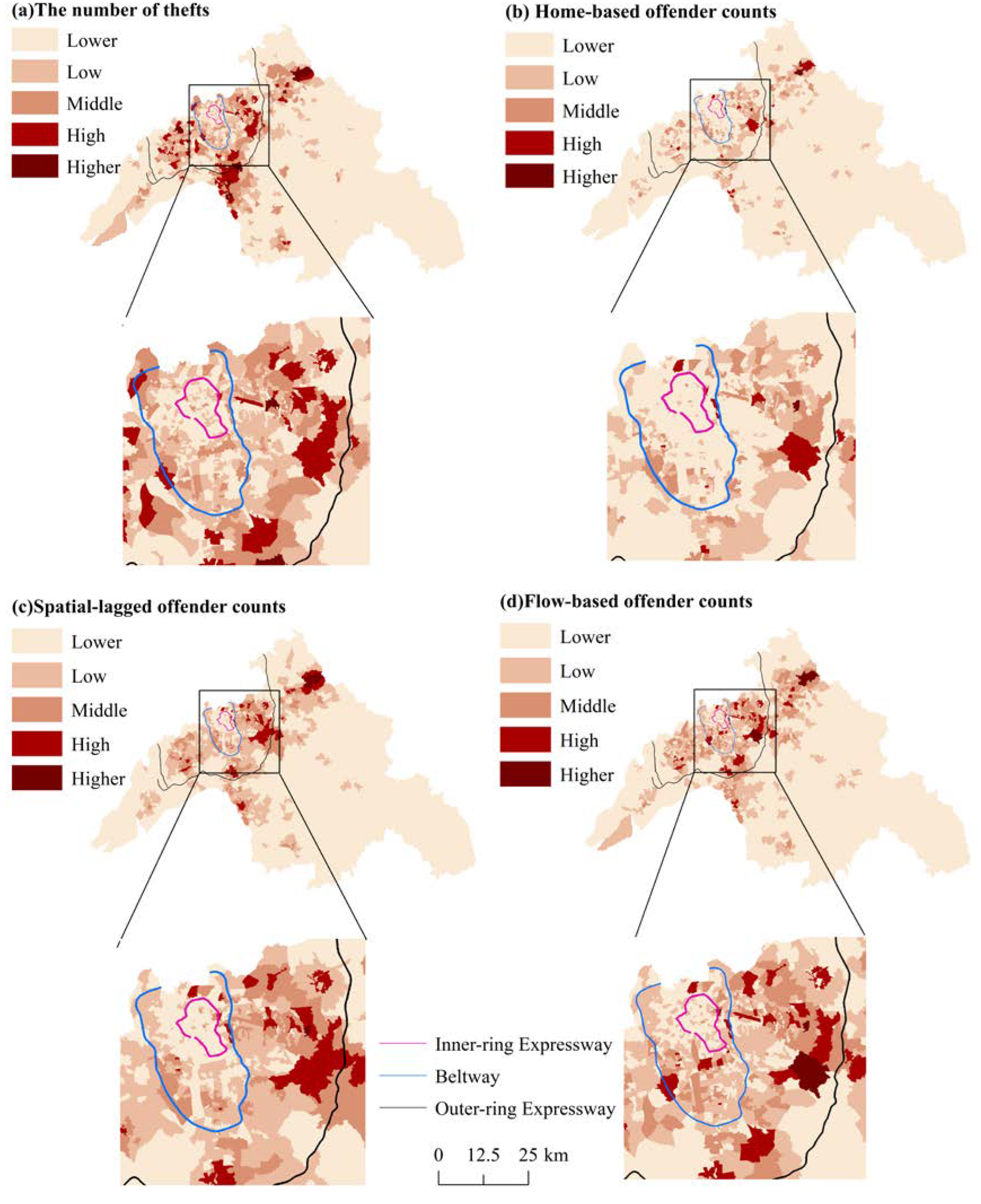
3.2. Spatial Distribution of Crime and Estimated Offenders

Although the estimated offender count using three different methods is significantly correlated with the number of thefts (Table 3), there are still differences in their spatial distribution.
Figure 2a shows the spatial distribution of thefts (the dependent variable) in ZG City, with a trend of low–high–low from the central urban area to the suburbs. The communities between the beltway and outer-ring expressway have the largest crime concentration. There were also crimes in the periphery of the outer-ring expressway. Communities within the inner-ring expressway, where the old towns are located, generally have fewer crimes. Figure 2b–d show the spatial distribution of offenders estimated with different methods (the independent variables). Figure 2b represents the spatial distribution of the home-based offender count in 2018, with a large concentration area between the beltway and outer expressway and another beyond the outer expressway. Figure 2c refers to the spatial distribution of the spatial-lagged offender count, and Figure 2d reflects the spatial distribution of the flow-based offender count. It is evident that the flow-based offender count (Figure 2d) captures more of offenders’ daily activity places than the home-based (Figure 2b) and spatial-lagged offender count methods (Figure 2c). Visual inspection also shows that the flow-based offender count matches theft better than the other two counts.

3.3. Results of Negative Binomial Regression Models

The likelihood ratio (LR) test shows that α is significantly not equal to zero (Table 4), confirming the overdispersion of crime counts. Therefore, the choice of the negative binomial model is supported. Chi-square tests show that the Chibar2 value of the three models is significant at 0.001, indicating that independent variables have a significant impact on the dependent variable. According to extant studies, a variance inflation factor (VIF) of independent variables lower than 10 indicates no obvious multicollinearity problem [10,14,45]. The maximum VIF values are less than 1.7 for all three models, thus alleviating the concern of multicollinearity. In addition, the Moran’s I values of the residuals for the three groups of models are equal to 0.000371, 0.000655, and 0.000908, respectively (p-value >0.05). Thus, no extra spatial autocorrelation should be handled.
Regarding the goodness of fit of the models, the flow-based offender count (Model 3) performed the best, followed by the spatial-lagged offender count (Model 2) and then the home-based offender count (Model 1). The standardized IRR value for the offender count variable increases from 1.334 (Model 1) to 1.465 (Model 2) to 1.629 (Model 3). These results confirm that the consideration of offender’s routine activities can help better explain crime.
The remaining independent variables have a significantly positive association with theft. By examining the standardized IRRs, bus stops, the proportion of the migrant population, and Internet bars have a stronger association than KTVs, subway stations, and cinemas. This finding is consistent across the three models.

4. Discussion and Conclusions

The routine activity theory emphasizes the importance of offenders’, residents’, as well as guardianships’ daily activities when analyzing crime. One assumption derived from the theory is that residents may be targeted by offenders not only in their home area, but also in their activity space. Similarly, offenders’ crime location choice should not be limited to their home area but also to inside their activity space, which is shaped by their daily activities.
Comparison of the AIC values among the three models shows a reduction of 96 from a starting value of 21,874.7 for Model 1 (home-based) to 21,778.3 for Model 2 (spatial-lagged), as well as a reduction of 28 from the starting value of 21,778.3 for Model 2 to 21,750.7 for Model 3 (flow-based). Since a greater reduction in AIC values indicates greater improvement in model performance, the improvement from the home-based model to the spatial-lagged model is greater than the improvement from the spatial-lagged model to the flow-based model. This result could infer that most offenders travel to their neighboring (spatial-lagged) areas more frequently than distant areas [15,30]. This is consistent with the distance decay pattern observed in the journey-to-crime literature [12,47,48,49,50].
The superior explanatory power of the flow-based offender counts underscores the importance of shifting the focus from offenders’ residential spaces to offenders’ activity spaces. Although the offenders are most familiar with their home location, they may not commit crime too close to home. This is termed the buffer zone effect [51]. This may be because the large number of acquaintances that act as informal controls in their living community present higher risk to offenders [51,52]. The visiting offenders from other communities do not face this problem. Such reduced risk can be an advantage of visiting offenders over the resident offenders.
The number of offenders estimated with the spatial-lagged method performed poorer than the flow-based method. It was stated earlier in the paper that 30% of thefts are committed by offenders who either live in the community or come from the immediate neighboring communities. However, convenient transportation such as buses, BRT systems, and subways facilitate long-distance journeys for potential offenders. The spatial-lagged method failed to capture such long-distance journeys, while the flow-based method captured all journeys to crime.
Consistent with the existing studies, the covariates, including bus stops, subway stations, Internet bars, KTVs, cinemas, and the proportion of the migrant population, all show significant positive impact on theft. The consistency with the literature enhances the validity of our research findings.
Although we verified that the flow-based offender count method outperformed the other methods, there are still some limitations in this study. Firstly, this study only considered arrested offenders in the analysis, while non-arrested offenders are ignored. One potential concern would be the representativeness of the arrested offenders. However, the 80–20 law states that most crimes are associated with a small number of offenders. The likelihood of repeat offenders being caught is very high. Therefore, the use of arrestee data can be acceptable, as is the common practice in the literature. Almost all crime location choice studies used arrested offenders when analyzing how offenders commit crimes. These studies suggest that the results of the analysis based on arrested offenders are sufficiently representative [15,53,54,55]. Secondly, individual differences between both residents and offenders in the same community was not taken into account. Further studies calculating residents’ and offenders’ flows could consider individual attributes such as age or gender. Thirdly, while we expect that the flow-based method is applicable to all crime types in which the journey-to-crime follows a distance decay pattern, its performance in relation to other crime types needs further validation. Fourthly, we did not examine the temporal pattern due to the sparsity of crime data. Future studies may consider flows linked to different routines and movements at different times of the day and days of the week.
In sum, the innovative flow-based offender count captures the routine activities of offenders. Compared to the traditional home-based offender count and the spatial-lagged offender count, the flow-based offender count can better explain crime. This new flow-based method is applicable to all cities, as long as intra-city flow data are available. This is an important contribution to the literature and also has practical implications. The flow-based method provides a viable way for the police department to predict the distribution of offenders in space. Thus, being able to estimate the locations of offender activities adds a new dimension for law enforcement agencies in the allocation of resources to areas with a higher concentration of offenders.

Author Contributions

Conceptualization, Lin Liu and Luzi Xiao; methodology, Chenchen Li and Guangwen Song; software, Chenchen Li and Luzi Xiao; validation, Lin Liu, Chenchen Li and Luzi Xiao; formal analysis, Chenchen Li and Luzi Xiao; data curation, Chenchen Li and Luzi Xiao; writing—original draft preparation, Lin Liu, Chenchen Li and Luzi Xiao; writing—review and editing, Lin Liu, Chenchen Li and Luzi Xiao; visualization, Chenchen Li; supervision, Lin Liu; funding acquisition, Chenchen Li, Luzi Xiao and Guangwen Song. All authors have read and agreed to the published version of the manuscript.

Funding

This work was supported by the National Natural Science Foundation of China (42001171, 42171218, 42071184), the Graduate Program of Guangzhou University (2022GDJC-M12), and the GuangDong Basic and Applied Basic Research Foundation (2023A1515011462).

Data Availability Statement

The data are not publicly available due to the confidentiality agreement with local police.

Conflicts of Interest

The authors declare no conflicts of interest.

References

  1. Cohen, L.; Felson, M. Social Change and Crime Rate Trends: A Routine Activity Approach. Am. Sociol. Rev. 1979, 44, 588–608. [Google Scholar] [CrossRef]
  2. Cohen, L.E. Modeling Crime Trends: A Criminal Opportunity Perspective. J. Res. Crime Delinq. 1981, 18, 138–164. [Google Scholar] [CrossRef]
  3. Brantingham, P.; Brantingham, P. Criminality of place: Crime generators and crime attractors. Eur. J. Offender Policy Res. 1995, 3, 5–26. [Google Scholar] [CrossRef]
  4. Song, G.; Liu, L.; Wim, B.; Xiao, L.; Zhou, S.; Liao, W. Testing Indicators of Risk Populations for Theft from the Person across Space and Time: The Significance of Mobility and Outdoor Activity. Ann. Am. Assoc. Geogr. 2018, 108, 1370–1388. [Google Scholar] [CrossRef]
  5. Brantingham, P.; Brantingham, P. Crime pattern theory. In Environmental Criminology and Crime Analysis; Wortley, R., Mazerolle, L., Eds.; Willan Publishing: London, UK, 2008; pp. 78–93. [Google Scholar]
  6. Chainey, S.P.; Matias, J.A.S.; Junior, F.C.F.N.; Silva, T.L.C.D.; Macêdo, J.A.F.d.; Magalhes, R.P.; Neto, J.F.d.Q.; Silva, W.C.P. Improving the Creation of Hot Spot Policing Patrol Routes: Comparing Cognitive Heuristic Performance to an Automated Spatial Computation Approach. Int. J. Geo-Inf. 2021, 10, 560. [Google Scholar] [CrossRef]
  7. Menting, B.; Lammers, M.; Ruiter, S.; Bernasco, W. The Influence of Activity Space and Visiting Frequency on Crime Location Choice: Findings from an Online Self-Report Survey. Br. J. Criminol. 2019, 60, 303–322. [Google Scholar] [CrossRef]
  8. Menting, B.; Lammers, M.; Ruiter, S.; Bernasco, W. Family Matters: Effects of Family Members’ Residential Areas on Crime Location Choice. Criminology 2016, 54, 413–433. [Google Scholar] [CrossRef]
  9. Kortas, F.; Grigoriev, A.; Piccillo, G. Exploring multi-scale variability in hotspot mapping: A case study on housing prices and crime occurrences in Heerlen. Cities 2022, 128, 103814. [Google Scholar] [CrossRef]
  10. Bernasco, W.; Block, R. Robberies in Chicago: A Block-Level Analysis of the Influence of Crime Generators, Crime Attractors, and Offender Anchor Points. J. Res. Crime Delinq. 2011, 48, 33–57. [Google Scholar] [CrossRef]
  11. Kurland, J.; Johnson, S.D.; Tilley, N. Offenses around Stadiums: A natural experiment on crime attraction and generation. J. Res. Crime Delinq. 2013, 51, 5–28. [Google Scholar] [CrossRef]
  12. Xiao, L.; Liu, L.; Song, G.; Ruiter, S.; Zhou, S. Journey-to-Crime Distances of Residential Burglars in China Disentangled: Origin and Destination Effects. Isprs Int. J. Geo Inf. 2018, 7, 325. [Google Scholar] [CrossRef]
  13. Bernasco, W. Adolescent offenders’ current whereabouts predict locations of their future crimes. PLoS ONE 2019, 14, e0210733. [Google Scholar] [CrossRef] [PubMed]
  14. Liu, L.; Sun, Q.; Xiao, L.; Song, G.w.; Chen, J. The temporal influence difference of drug-related personnels’ routine activity on the spatial pattern of theft. J. Geo-Inf. Sci. 2021, 23, 2187–2200. [Google Scholar]
  15. Song, G.; Yanji, Z.; Bernasco, W.; Cai, L.; Liu, L.; Qin, B.; Chen, P. Residents, Employees and Visitors: Effects of Three Types of Ambient Population on Theft on Weekdays and Weekends in Beijing, China. J. Quant. Criminol. 2021, 39, 385–423. [Google Scholar] [CrossRef] [PubMed]
  16. Bernasco, W.; Block, R.; Ruiter, S. Go where the money is: Modeling street robbers’ location choices. J. Econ. Geogr. 2012, 13, 119–143. [Google Scholar] [CrossRef]
  17. Rossmo, D.K.; Lu, Y.; Fang, T. Spatial-temporal crime paths. In Patterns, Prevention, and Geometry of Crime; Andresen, M.A., Kinney, J.B., Eds.; Routledge: New York, NY, USA, 2012; pp. 16–42. [Google Scholar]
  18. Griffiths, G.; Johnson, S.; Chetty, K. UK-based Terrorists’ Antecedent Behaviour: A Spatial and Temporal Analysis. Appl. Geogr. 2017, 86, 274–282. [Google Scholar] [CrossRef]
  19. Zhou, S.; Deng, L.; Kwan, M.P.; Yan, R. Social and spatial differentiation of high and low income groups’ out-of-home activities in Guangzhou, China. Cities 2015, 45, 81–90. [Google Scholar] [CrossRef]
  20. Tu, P.; Yao, W.; Zhao, Z.; Wang, P.; Wu, S.; Fang, Z. Interday Stability of Taxi Travel Flow in Urban Areas. ISPRS Int. J. Geo-Inf. 2022, 11, 590. [Google Scholar] [CrossRef]
  21. Qian, Z. Travel Behavior of Residents in Transit-Oriented Development (TOD) Neighborhoods: A Study of Two Neighborhoods in Shenzhen, China. In Urban Transformational Landscapes in the City-Hinterlands of Asia: Challenges and Approaches; Springer Nature: Singapore, 2023; pp. 41–53. [Google Scholar]
  22. Mao, Y.; Ding, J. Study on Spatial-temporal Partterns of Robbery and Snatch: A Case Study of Pidong New Area, Shanghai. Hum. Grography 2014, 29, 49–54. [Google Scholar] [CrossRef]
  23. Qin, X.; Liu, L. Evaluating the Relationships of Bus Transit with Street and Off-Street Robberies. Prof. Geogr. 2015, 68, 227–237. [Google Scholar] [CrossRef]
  24. Li, J.; Song, G.; Xiao, L.; Zhang, X. Characteristics and influencing factors of thieves’travel distance: A comprehensive consideration of residential community, target community, and physical barriers to travel. Prog. Geogr. 2022, 41, 2123–2134. [Google Scholar] [CrossRef]
  25. Sun, D.; Dan, B. Impact of urban built environment on residential choice of commuting mode in Shanghai. Acta Geogr. Sin. 2015, 70, 1664–1674. [Google Scholar]
  26. Shao, H.; Jin, C.; Zhong, Y.; Mao, W. The impact of Haikou’s urban built environment on online car-hailing during peak hours: Based on DIDI travel data. Hum. Geogr. 2022, 37, 130–139. [Google Scholar] [CrossRef]
  27. Zhao, Z.; Liu, D.; Xiao, J.; Wang, S. Spatial characteristics and influencing factors analysis of journey-to-crime based on crime pattern theory: A study of theft crime in Nanguan District, Changchun. Geogr. Res. 2021, 40, 885–899. [Google Scholar]
  28. Wiles, P.; Costello, A. The ‘road to nowhere’: The evidence for travelling criminals. In Principles of Geographical Offender Profiling; Home Office Research Study 207, Research, Development and Statistics Directorate, Home Office; Routledge: London, UK, 2000; pp. 1–12. [Google Scholar]
  29. Gabor, T.; Gottheil, E. Offender Characteristics and Spatial Mobility: An Empirical Study and Some Policy Implications. Can. J. Criminol. Rev. Can. Criminol. 1984, 26, 267–281. [Google Scholar] [CrossRef]
  30. Song, G.; Bernasco, W.; Liu, L.; Xiao, L.; Zhou, S.; Liao, W. Crime Feeds on Legal Activities: Daily Mobility Flows Help to Explain Thieves’ Target Location Choices. J. Quant. Criminol. 2019, 35, 831–854. [Google Scholar] [CrossRef]
  31. Chen, J.; Liu, L.; Zhou, S.; Xiao, L.; Jiang, C. Spatial Variation Relationship between Floating Population and Residential Burglary: A Case Study from ZG, China. ISPRS Int. J. Geo-Inf. 2017, 6, 246. [Google Scholar] [CrossRef]
  32. Xiao, L.; Ruiter, S.; Liu, L.; Song, G.; Zhou, S. Burglars blocked by barriers? The impact of physical and social barriers on residential burglars’ target location choices in China. Comput. Environ. Urban Syst. 2021, 86, 101582. [Google Scholar] [CrossRef]
  33. Yue, H.; Liu, L.; Luzi, X. Investigating the effect of people on the street and streetscape physical environment on the location choice of street theft crime offenders using street view images and a discrete spatial choice model. Appl. Geogr. 2023, 157, 103025. [Google Scholar] [CrossRef]
  34. Xu, C.; Luzi, X.; Song, G.; Pan, B.; Liu, H. The impact of community residents’ occupational structure on the spatial distribution of different types of crimes. Habitat Int. 2021, 117, 102435. [Google Scholar] [CrossRef]
  35. Conrow, L.; Aldstadt, J.; Mendoza, N.S. A spatio-temporal analysis of on-premises alcohol outlets and violent crime events in Buffalo, NY. Appl. Geogr. 2015, 58, 198–205. [Google Scholar] [CrossRef]
  36. Hong, J.; Huang, L. A split and swaying approach to building information society: The case of Internet cafes in China. Telemat. Inform. 2005, 22, 377–393. [Google Scholar] [CrossRef]
  37. Lan, M. Examining the Impact of Bus Stop Location Change on Robbery. Master’s Thesis, University of Cincinnati, Cincinnati, OH, USA, 2016. [Google Scholar]
  38. Xiao, L.; Liu, L.; Zhou, S.; Song, G.; Zhang, C.; Chen, J. Spatio-temporal Pattern of Pickpocketing at Subway Stations on Weekdays of ZG City and Its Influencing Factors. Sci. Geogr. Sin. 2018, 38, 1227–1234. [Google Scholar]
  39. Chen, Q. Advanced Econometrics and Stata Applications, 2nd ed. The sort and count models; Higher Education Press: Beijing, China, 2014; pp. 211–213. [Google Scholar]
  40. Berk, R.; MacDonald, J. Overdispersion and Poisson Regression. J. Quant. Criminol. 2008, 24, 269–284. [Google Scholar] [CrossRef]
  41. Land, K.; McCall, P.; Nagin, D. A Comparison of Poisson, Negative Binomial, and Semiparametric Mixed Poisson Regression Models: With Empirical Applications to Criminal Careers Data. Sociol. Methods Res. 1996, 24, 387–442. [Google Scholar] [CrossRef]
  42. Xiao, L.; Liu, L.; Song, G.; Zhou, S.; Long, D.; Feng, J. Impacts of community environment on residential burglary based on rational choice theory. Geogr. Res. 2017, 36, 2479–2491. [Google Scholar]
  43. Chen, Q. Advanced Econometrics and Stata Applications, 2nd ed. Model settings and data issues; Higher Education Press: Beijing, China, 2014; pp. 118–119. [Google Scholar]
  44. Xu, C.; Yang, Y.; Song, G.; Liu, L.; Lan, M.; Chen, X. The impact of civil registration-based demographic heterogeneity on community thefts. Habitat Int. 2022, 129, 102673. [Google Scholar] [CrossRef]
  45. Chen, Q. Advanced Econometrics and Stata Applications, 2nd ed.; Model Settings and Data Issues; Higher Education Press: Beijing, China, 2014; pp. 123–124. [Google Scholar]
  46. Shrestha, N. Detecting multicollinearity in regression analysis. Am. J. Appl. Math. Stat. 2020, 8, 39–42. [Google Scholar] [CrossRef]
  47. Johnson, L.T.; Taylor, R.B.; Ratcliffe, J.H. Need drugs, will travel?: The distances to crime of illegal drug buyers. J. Crim. Justice 2013, 41, 178–187. [Google Scholar] [CrossRef]
  48. Levine, N.; Lee, P. Journey-to-Crime by Gender and Age Group in Manchester, England. In Crime Modeling and Mapping Using Geospatial Technologies; Springer: Dordrecht, The Netherlands, 2013; pp. 145–178. [Google Scholar]
  49. Ackerman, J.; Rossmo, D. How Far to Travel? A Multilevel Analysis of the Residence-to-Crime Distance. J. Quant. Criminol. 2014, 31, 237–262. [Google Scholar] [CrossRef]
  50. Andresen, M.; Frank, R.; Felson, M. Age and the distance to crime. Criminol. Crim. Justice 2014, 14, 314–333. [Google Scholar] [CrossRef]
  51. Bernasco, W.; Nieuwbeerta, P. How do residential burglars select target areas?: A New Approach to the Analysis of Criminal Location Choice. Br. J. Criminol. 2005, 4, 296–315. [Google Scholar] [CrossRef]
  52. Ozer, M.; Onat, I.; Akbas, H.; Elsayed, N.; Elsayed, Z.; Varlioglu, S. Exploring the Journey to Drug Overdose: Applying the Journey to Crime Framework to Drug Sales Locations and Overdose Death Locations. arXiv 2023, arXiv:2305.19859. [Google Scholar]
  53. Bernasco, W. Modeling Micro-Level Crime Location Choice: Application of the Discrete Choice Framework to Crime at Places. J. Quant. Criminol. 2010, 26, 113–138. [Google Scholar] [CrossRef]
  54. Johnson, S.; Summers, L. Testing Ecological Theories of Offender Spatial Decision Making Using a Discrete Choice Model. Crime Delinq. 2015, 61, 454–480. [Google Scholar] [CrossRef]
  55. Lammers, M.; Menting, B.; Ruiter, S.; Bernasco, W. Biting Once, Twice: THE Influence of Prior on Subsequent Crime Location Choice. Criminology 2015, 53, 309–329. [Google Scholar] [CrossRef]
Figure 1. An example of the number of offenders estimated with the flow-based method.
Ijgi 13 00008 g001
Figure 2. Spatial distribution of thefts and estimated offender count.
Ijgi 13 00008 g002
Table 1. Sample of people’s trajectory data from the DAAS platform of Unicom.
O_CodeD_CodeO_PtypeD_PtypeCount
440113105202440106011029122
440113105202440111103221202
440113105202440111002004101
4401131052024401060220060158
440113105202440106021006204
440113105202440106017010104
4401131052024401060090060017
...............
Table 2. Descriptive statistics of the variables.
VariablesMeanVarianceMinMaxCoefficient of Variation
The number of thefts36.392 61.110 09290.215
The number of offenders estimated:
Home-based offender count (V1)1.4844.0310661.353
Spatial-lagged offender count (V2)3.6776.072083.40.670
Flow-based offender count (V3)35.34866.6501096.320.231
Bus stops2.5443.98901020.785
Subway stations0.0470.2310310.226
Internet bars1.1022.2080241.348
KTVs0.5151.3290162.238
Cinemas0.1990.7770104.430
Migrant population (%)0.2700.23700.9741.803
Table 3. Correlation analysis of the variables.
VariablesTheft(V1)(V2)(V3)Bus StopsSubway StationsInternet BarsKTVsCinemasMigrant Population (%)
Theft1
(V1)0.626 ***1
(V2)0.672 ***0.841 ***1
(V3)0.778 ***0.854 ***0.824 ***1
Bus stops0.584 ***0.317 ***0.374 ***0.500 ***1
Subway stations0.205 ***0.082 ***0.087 ***0.218 ***0.170 ***1
Internet bars0.595 ***0.363 ***0.414 ***0.444 ***0.326 ***0.123 ***1
KTVs0.517 ***0.301 ***0.343 ***0.430 ***0.304 ***0.170 ***0.506 ***1
Cinemas0.358 ***0.121 ***0.147 ***0.277 ***0.232 ***0.270 ***0.361 ***0.390 ***1
Migrant population (%)0.395 ***0.312 ***0.410 ***0.368 ***0.336 ***0.048 *0.326 ***0.218 ***0.088 ***1
Notes: * p < 0.05, ** p < 0.01, *** p < 0.001; (V1) represents the home-based offender count; (V2) refers to the spatial-lagged offender count; and (V3) is the flow-based offender count.
Table 4. Results from negative binomial regression models with different offender estimation methods.
VariablesModel 1 (Home-Based)Model 2 (Spatial-Lagged)Model 3 (Flow-Based)
StandardizedUnstandardizedStandardizedUnstandardizedStandardizedUnstandardized
IRRcoef.IRRcoef.IRRcoef.IRRcoef.IRRcoef.IRRcoef.
Offenders1.334 0.288 ***1.074 0.072 ***1.465 0.382 ***1.065 0.063 ***1.629 0.488 ***1.007 0.007 ***
Bus stops1.510 0.412 ***1.109 0.103 ***1.444 0.367 ***1.096 0.092 ***1.370 0.315 ***1.082 0.079 ***
Subway stations1.115 0.109 ***1.603 0.472 ***1.123 0.116 ***1.655 0.504 ***1.076 0.073 ***1.372 0.316 ***
Internet bars1.272 0.241 ***1.115 0.109 ***1.243 0.218 ***1.104 0.099 ***1.251 0.224 ***1.107 0.101 ***
KTVs1.129 0.121 ***1.096 0.091 ***1.117 0.111 ***1.087 0.083 ***1.098 0.094 ***1.073 0.070 ***
Cinemas1.109 0.103 ***1.142 0.133 ***1.106 0.100 ***1.138 0.129 ***1.078 0.076 ***1.102 0.097 ***
Migrant population (%)1.388 0.328 ***3.993 1.385 ***1.333 0.288 ***3.372 1.215 ***1.341 0.293 ***3.452 1.239 ***
Chi-square2062.47 ***2158.94 ***2186.48 ***
α0.798 ***0.767 ***0.760 ***
Max VIF1.591.601.67
AIC21,874.721,778.321,750.7
BIC21,927.721,831.221,803.7
Notes: * p < 0.1, ** p < 0.05, *** p < 0.01.
Disclaimer/Publisher’s Note: The statements, opinions and data contained in all publications are solely those of the individual author(s) and contributor(s) and not of MDPI and/or the editor(s). MDPI and/or the editor(s) disclaim responsibility for any injury to people or property resulting from any ideas, methods, instructions or products referred to in the content.

