Article

Multi-Session High-Definition Map-Monitoring System for Map Update

1
School of Vehicle and Mobility, Tsinghua University, Beijing 100084, China
2
Department of Industrial Engineering, Tsinghua University, Beijing 100084, China
*
Author to whom correspondence should be addressed.
These authors contributed equally to this work.
ISPRS Int. J. Geo-Inf. 2024, 13(1), 6; https://doi.org/10.3390/ijgi13010006
Submission received: 26 July 2023 / Revised: 9 December 2023 / Accepted: 18 December 2023 / Published: 22 December 2023

Abstract

:
This research paper employed a multi-session framework to present an innovative approach to map monitoring within the domain of high-definition (HD) maps. The proposed methodology uses a machine learning algorithm to derive a confidence level for the detection of specific map elements in each frame and tracks the position of the element in subsequent frames. This creates a virtual belief system, which indicates the existence of the element on the HD map. To confirm the existence of the element and ensure the credibility of the map data, a reconstruction and matching technique was implemented. The notion of an expected observation area is also introduced by strategically limiting the vehicle’s observation range, thereby bolstering the detection confidence of the observed map elements. Furthermore, we leveraged data from multiple vehicles to determine the necessity for updates within specific areas, ensuring the accuracy and dependability of the map information. The validity and practicality of our approach were substantiated by real experimental data, and the monitoring accuracy exceeded 90 % .

1. Introduction

With the increasing dependency on high-definition (HD) maps for the development of intelligent vehicle (IV) technology [1,2,3], it is now more important than ever to achieve an up-to-date, reliable, and accurate map [4,5]. The information provided by the HD map can lead to more-reliable decisions for planning and control since the optimal routes can be determined in an instant. In perception tasks, the drivable area and lane information can be utilized to detect the vehicle position by exploiting visual cues such as traffic signs, road markers, and lanes [6,7]. In recent years, researchers have built HD maps from aerial images [8]. However, the state-of-the-art method to create HD maps relies on specialized vehicles equipped with sophisticated sensors such as light detection and ranging (LiDAR) and the real-time kinematic positioning-global navigation satellite system (RTK-GNSS) [9]. These vehicles are expensive, which limits the number of mapping vehicles dispatched on the road [10].
In our everyday lives, dynamic changes occur in the road environment. For example, lane lines can be removed when the road is coated with new asphalt; arrow markers on the road can differ due to local regulation changes; centerlines can be moved for the expansion of the lane width. These add to the number and complexity of tasks that need to be performed by specialized mapping vehicles. Previously, whenever a map needed to be updated, the specialized mapping vehicle will update the map as a whole. As a result of the high workload during an update, the frequency of updates in the necessary areas are relatively low [11]. To avoid the ineffective allocation of resources and reduce the burden of performing these map updates, specialized mapping vehicles should only be dispatched to areas that require updates on the map [
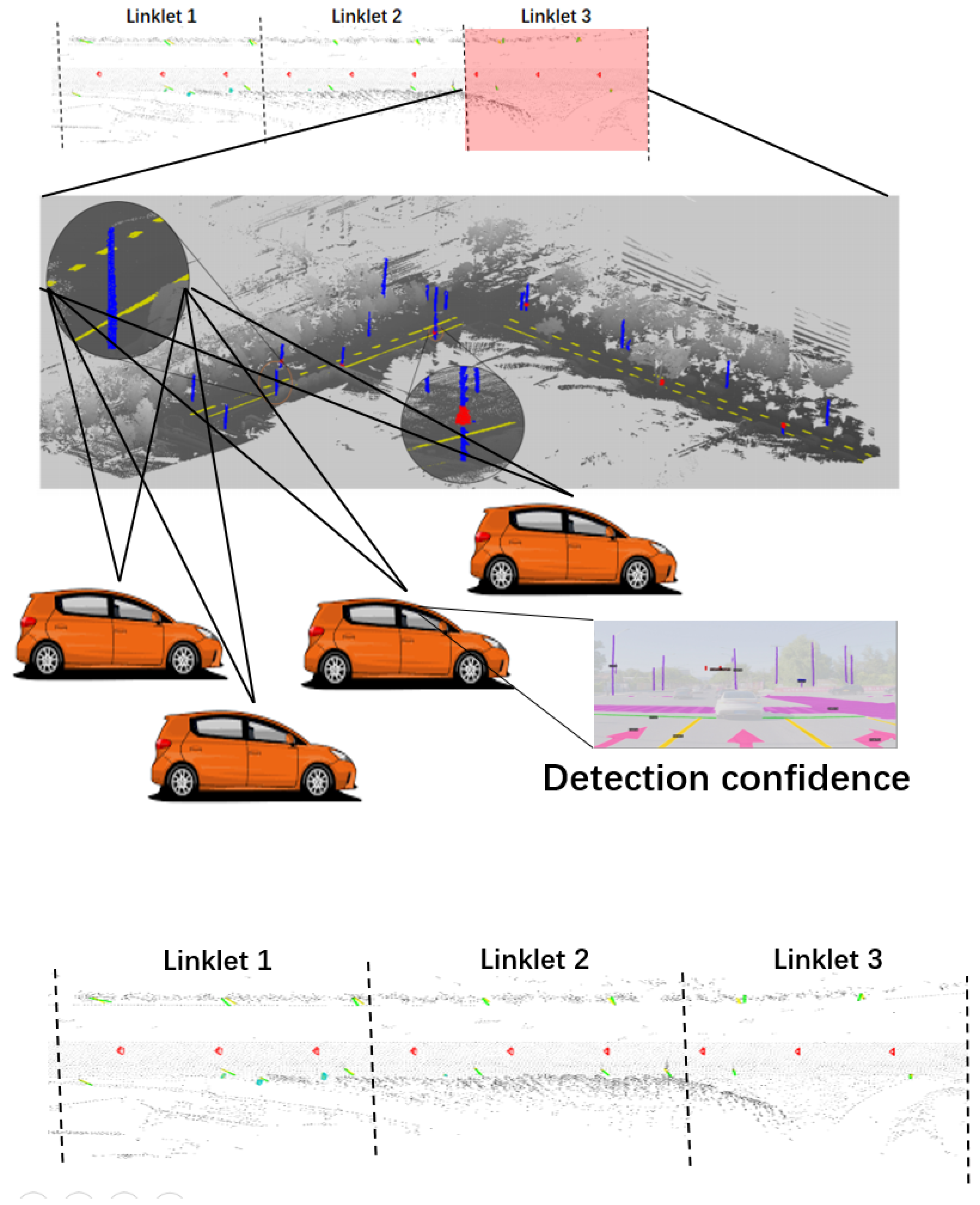
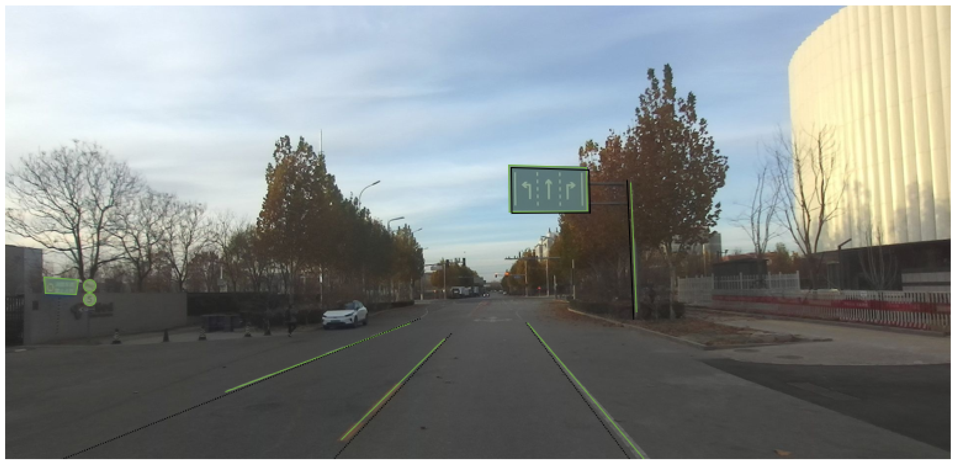
12]. In this paper, we aimed to identify these specific out-of-date areas by outsourcing the detection of changes to the road environment to mass-produced vehicles equipped with low-cost sensors such as monocular cameras and GNSS. The visualization of the monitoring system can be seen in Figure 1.
Conventional map-change-detection methods will typically project the map data, such as traffic poles, road markings, and lane lines into the 2D image and perform a matching algorithm to determine whether the change has occurred [13]. Pannen et al. performed change detection using a boosted particle filter trained using datasets to update lane lines with crowdsourced data [14]. This approach utilized multiple sessions or multiple transversals, which outperformed single-session change detection. The phrase ‘multi-session’ denotes multiple visits by one or more vehicles to a specific area, exceeding one visit, while ‘single session’ describes a one-time visit by a single vehicle to a particular area in order to determine the change.
In another study, a simultaneous localization and map change update (SLAMCU) was proposed to perform the simultaneous localization and mapping (SLAM) algorithm and HD map update at the same time [15]. This method relies on expensive LiDAR sensors to determine the change, which means the solution might not be viable in the near future given the high cost of LiDAR on the market. In 2020, Pannen et al. introduced a new method of performing map updates by utilizing density-based clustering of applications with noise (DBSCAN) [16]. In this method, only the vectorized map data are considered, and the system does not differentiate good and bad information. Ref. [17] proposed a novel method to detect map change based on deep metric learning, which projects the existing map data into the image domain, directly compares it to the detected map element, and calculates a similarity score. Although this approach is a great breakthrough since it only uses a single frame in the change-monitoring algorithm, the system lacks robustness toward occlusion and false detection cases.
In this study, we combined the advantages of single-session map monitoring, which is rich in semantic information, with multi-session map monitoring, where more information can be used to determine the map change. A confidence level is assigned to each map element to determine how confident the system is about the existence of the map element [18]. For map elements with a confidence level above a predetermined threshold, map matching is performed on the vehicle side, and the results are sent to the server to monitor the HD map as a whole.
The foremost contributions of this paper are:
  • Formulating a map element confidence level model based on map element detection accuracy observed in a series of occupancy objects.
  • Proposing a systematic approach to create a multi-session HD map-monitoring system from the aggregation of multiple single-session HD map-monitoring results.
  • Conducting experiments based on real-world data. The results demonstrated the effectiveness and efficiency of the proposed method.
This paper is organized as follows: Section 2 of this paper discusses the related work in the extant literature. In Section 3, the single-session map monitoring approach is introduced. The aggregation of single-session map monitoring results to obtain a multi-session map monitoring system is described in Section 4. The model is applied to a real case scenario in Section 5, which also discusses the technical challenges encountered in the implementation. Finally, the conclusion of the study is drawn in Section 6.

2. Related Work

2.1. Crowdsourced HD Map Update

In the past few years, much work has gone into making public map updates better so that map features can be added, taken away, or moved. Liu used the Kalman filter to obtain information about conceptual certainty and to join the positions of map elements [4]. This method is slow because it changes over time and works in steps. Liebner used a graph-based method and SLAM optimization to make smooth shapes in the new map [19]. Even though this method has a mean absolute distance error of about 30 cm when it comes to lane marking variation, it needs much computing power when it comes to thousands of shared data. Chao solved the problem by increasing the quality of the map and the state of each map piece based on how well they matched the route [20]. This method emphasizes the map’s surface data more than the vertical map elements, so the result of the update may be incomplete and non-ideal. Ref. [21] used bus and taxi data in Seoul to perform HD map updates for on-surface map elements. Although the theoretical basis was laid out and the proof of concept to perform map updates through crowdsourced data was given, the map quality resulting from this method still remains the main concern.

2.2. HD Map Change Detection

To mitigate inaccuracies in map updates derived from crowdsourced data, some researchers have chosen to employ crowdsourced data exclusively for the purpose of detecting changes. They then utilize specialized mapping vehicles to perform the actual update, thereby guaranteeing the integrity and quality of the map update, while simultaneously addressing the concern regarding the low map update frequency, as mentioned in the previous section.
Jo et al. used the Dempster–Shafer (DS) evidence theory to evaluate HD map features to measure map change [15]. Heo and colleagues used direct deep metric learning, which projects the HD map into the image space. To determine the change, the projected map and detected map element are compared and a similarity score is calculated [17]. Lambert and Hays proposed a trust but verify (TbV) dataset to train a learning-based algorithm to detect HD vector map changes [22]. Zhang et al. implemented a real-time HD map-change-detection method for crowdsourced updates using mid- to high-end sensors, such as an industry camera, a high-end GNSS and inertial measurement unit (IMU), and an onboard computing platform [23]. They used the random sample consensus (RANSAC) algorithm [24] to match the detected features with the map using a matching degree coefficient based on map element overlap. However, these single-session change-detection methods cannot directly exclude semi-static objects (e.g., parked cars) from sensor measurements, and as a result, they are not able to verify the map element obstructed by these semi-static objects. Due to the intelligent vehicle’s observation bias, these methods will misdetect the map changes.
Multi-session change detection can reduce observation bias caused by the sensor’s limited field of view. Map modification usually depends on confidence; in a 2019 study conducted by Pannen et al., the mean particle weight, belief weight, mean inner lane geometry innovation, and mean lane geometry weight determine the solution quality of map feature localization [14]. In subsequent iterations, Ref. [16] proposed using the linklet criteria to partition the map topology into links and vertices to locate the change. They used floating car data (FCD) from existing vehicles to update the HD map data and proposed a regressor algorithm to calculate the change probability from the ground truth training dataset. Li et al. used crowdsourced images from multi-session vehicle trajectories to detect lane marking changes [25]. The confidence was modeled based on a Bayesian model with a Gaussian belief function distribution. Kim et al. used LiDAR-equipped crowdsourced vehicles to detect change [26]. They proposed a probabilistic and evidential method to update the existence field of point cloud points and matched them with the map to label them as existing, new, or deleted. Most of these approaches would require the raw data, which will impose a heavy burden on the server that aggregates all of the crowdsourced data.

3. Single-Session Monitoring

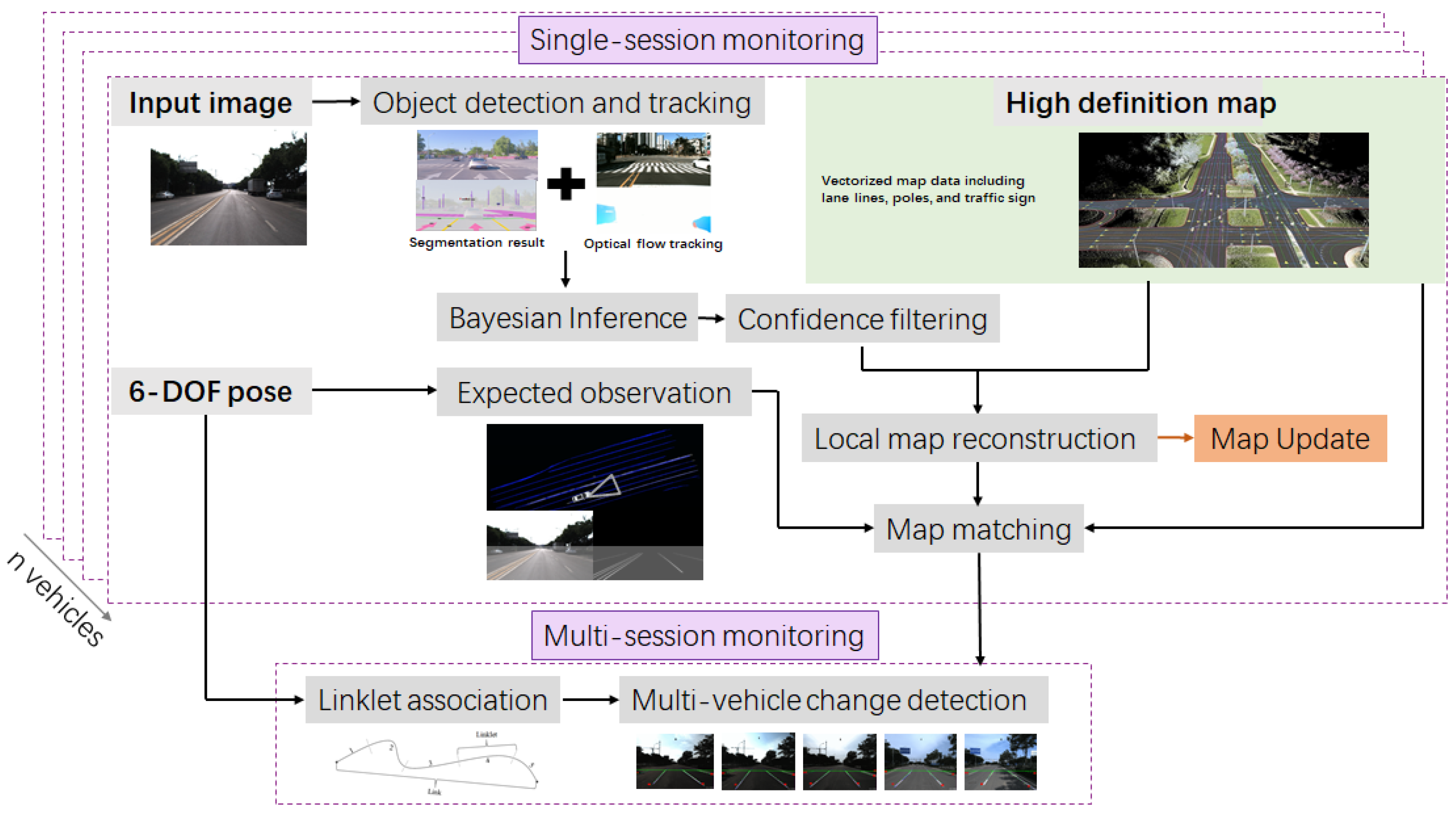
In this section, we describe the system model and the workflow for a single-session monitoring framework. This model is based on a reporting system on the vehicle side that will be transferred to the server side. However, the absolute decision as to whether the map has been changed or not should be based on the multi-session framework since it is richer in information. The whole framework can be seen in Figure 2.

3.1. Map Object Detection and Tracking

For map object detection, we used the classic region-based convolutional neural network (R-CNN) algorithm called MaskRCNN because of its robustness to create an instance and bounding box with confidence values [27] for pole-like objects, as well as traffic signs. Note that the network only helps to create segmentation results. Thus, further post-processing steps are required. For pole-like objects, the center pixels for the top and bottom boundary of the mask are defined as the control points. As for signs, the Hough transform was used to determine the control points from the outer contours. For lane line detection, we utilized the algorithm proposed in [28]. Similar to the previous objects, a further post-processing step is required to vectorize the instance segmentation results into a set of control points, which are separated according to the length between the points. It is important to note that the network was also further optimized with the labeled dataset collected in the same test area to enhance detection accuracy.
After we were able to detect the map element, the main challenge was to perform multi-object tracking for different map elements. The time at which a map element is first detected is denoted as t = t 1 , and the time at which the same map element is last detected is denoted as t = T . Considering that we are tracking many map elements, which are either vertically positioned, such as pole-like objects and signs, or horizontally positioned, such as lane markers, it is better to track the object in the image space. Using the traditional method can lead to a very big error caused by distortions in perspective. Furthermore, the wrong association between tracked map elements can lead to confidence error, which might be significant for the monitoring result. Here, we used a state-of-the-art dense optical flow algorithm called recurrent all-pairs field transform (RAFT) [29], which gives the corresponding distance between tracked pixels of two consecutive frames. Given that the detection m t i M t and m t 1 i M t 1 , the distance between m t i and the pixel prediction of the previous frame m t 1 j can be calculated by warping the optical flow estimation of g t 1 . The warping process uses the motion vector obtained from optical flow estimation for every pixel to locate the position of each pixel in the next frame. The formula of the warping process can be seen in [30].
g f l o w = warp ( g t 1 , m t 1 j ) , m t i
The map element association between two time frames is performed by finding the minimum Manhattan distance between the previous prediction and the detected map object in the next time frame. When the predicted pixel locations of the vertical objects (poles and signs) are outside of the image border A = ( 0 , A ) ( W A , W ) and the ground objects (lane lines) are outside of the image horizon B = ( 0 , B ) , the tracking of that element is finished. The visualization of this limit can be seen in Figure 3.
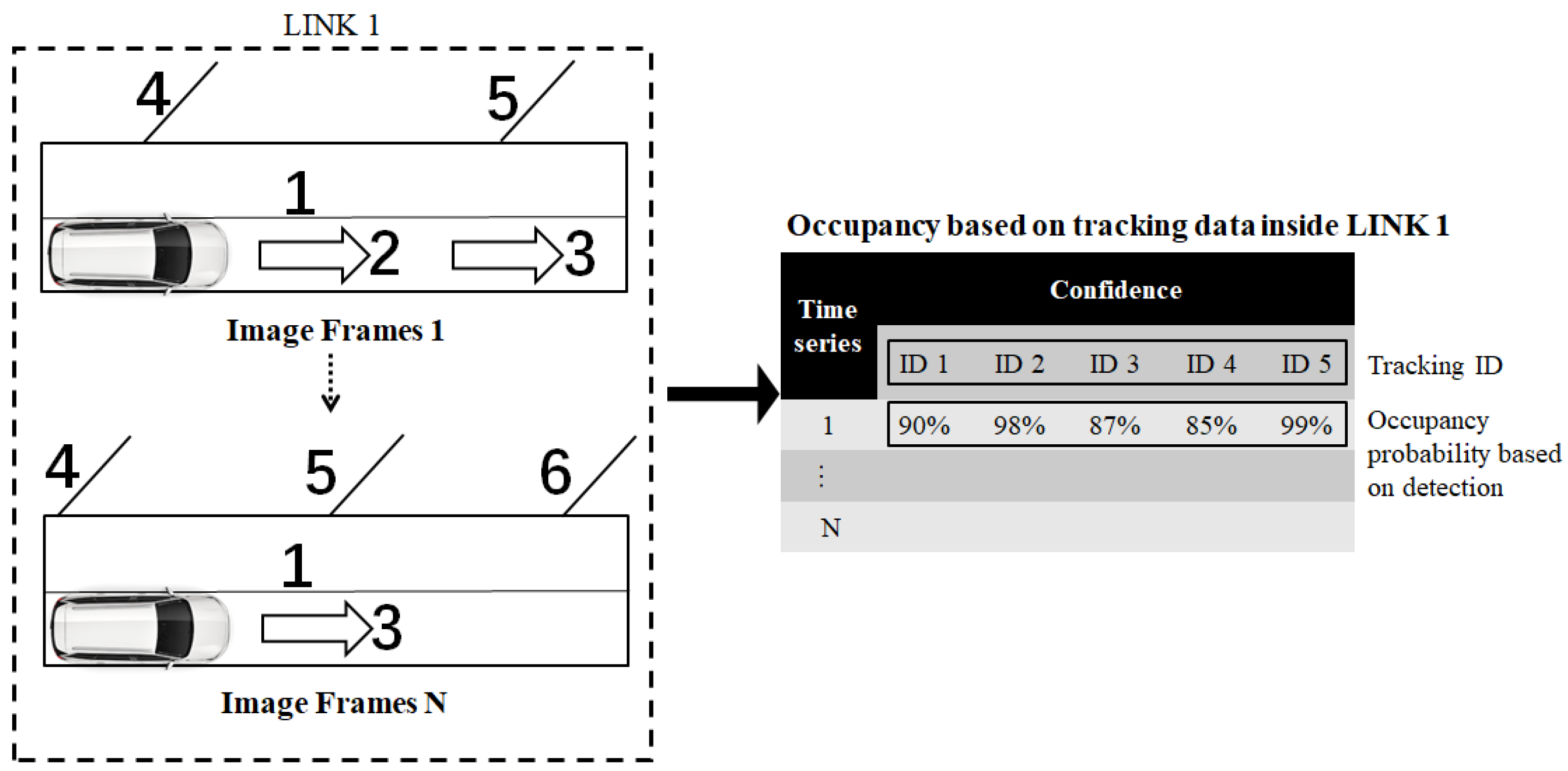
When the detected map element is registered as tracked, we put the confidence value inside an occupancy object table in a time series manner O t = t 1 : T as z i t . It is important to note that, for the case of missing tracking, the occupancy table is also filled with z i t = 0 . The observation of the map element in the image plane is modeled as a series of occupancy objects, as shown in Figure 4. This occupancy object works as an occupancy grid, but instead of using the grid as a reference, we used the map element itself as the reference. These occupancy objects will be used in the next step when we want to calculate the existence confidence of the map element.

3.2. Bayesian Recursion Confidence

After we have collected the occupancy object of the map element, the next step is to estimate the state of map elements using multiple frame observations. The posterior probability of the map element is estimated by a series of observations collected on the occupancy object. It is given that
X i t = 1 , m i exists , 0 , m i does not exist
For the observation of each frame, it is natural to have cases where missed detections and false detections occur. These two perceptual errors are also the main source of noise in z i t . Here, we introduced the missed detection probability P m and false detection probability P f of image perception. The former gives rise to:
P ( X i t | exists ) = P m 1 z i t ( 1 P m ) z i t
and the latter gives rise to:
P ( X i t | does not exist ) = P f z i t ( 1 P f ) 1 z i t
when false detection occurs and missed tracking happens. Then, P ( X i t = 1 | Z t 1 : T ) represents the probability that there is a map element observed in the map from t = t 1 to t = T .
P ( T t ) = t p ( T ) d T = 1 F T ( t )
where p ( T ) is the probability density function of the map element and F T ( t ) is the accumulation of the p ( T ) distribution function.
According to the Bayesian inference formula, we have:
P ( X i t = 1 | Z i t 1 : T ) = P ( Z i t 1 : T | T t ) P ( T t ) P ( Z i t 1 : T )
P ( Z i t 1 : T | T ) = t T P m 1 z i t ( 1 P m ) z i t t > T P f z i t ( 1 P f ) 1 z i t
P ( Z i t 1 : T ) = n = 0 N P ( Z i t 1 : T | k n ) F T ( k n + 1 ) F T ( k n )
The probability density function of T represents the statistical characteristics of the map elements in the macro sense, i.e., the frequency of map element changes. The time probability density of a typical event’s occurrence can be modeled by an exponential distribution function, which describes the probability distribution of the time interval T from the current observation to the moment when the map elements change. In this paper, we simplified the modeling of the probability density function by assuming that the current change time of a map element is 0 or does not change ( T = ). That is,
p ( T ) = f λ ( T ) = λ exp ( λ T ) , T 0 0 , T < 0
p ( T ) = K δ ( T ) + 1 K lim t δ ( T t )
where K represents the prior probability of the existence of a map feature.
However, since the ending of the time series for each tracked element varies and is unknown in practice, a threshold value for the number of times a map element is observed has to be satisfied in order to have reliable confidence. In this paper, we call this variable N , and only when the elements have more than N observations can the obtained posterior probability be used as the confidence to judge whether the map element exists or not in reality. We set this threshold value to be 8 to satisfy the posterior probability ϵ ( 0 , 1 ) and also set the threshold of probability to 0.8 to ensure the existence is true.

3.3. Map Reconstruction

After the confidence of the map element has been calculated, the next step is to reconstruct the map element that we believe to exist in a 3D space. The vehicle pose used in this paper was derived from GNSS and the IMU. It is important to note that the reconstruction problems for lane-like elements and pole-like elements are different. Here, we briefly describe the approach we chose to take for this step:
Lane reconstruction: The lane was reconstructed from the projection of the bird’s-eye view (BEV) by inverse projection mapping (IPM). Given the camera and installation poses { v R c , v t c } for the vehicle, the 3D lane marking can be reconstructed in the local coordinate with the assumption of a flat road as:
p v l = v t c z v R c p i z p i
where p v l denotes the 3D lane markings of a fixed road surface height in the vehicle local coordinate and p i denotes the 2D lane markings in the normalized 2D image plane obtained from the detection result of m t l . This process is performed to transform the information in the pixel coordinate into the vehicle coordinate. When the vehicle pose x is defined as a 6-DoF pose { R , t } , we can map p v l into a global coordinate M w l = { p w l } R 3 by:
p w l = R · p v l + t
The lane ID separation is obtained from the tracking. When the tracking is finished, the lane ID is considered finished as well, and we can add 1 to the lane ID index.
Poles’ reconstruction: Given the camera projection matrix K and the camera pose x = ( w R c , w t c ) , the projection of the Plücker coordinate of 3D line L w k = ( n w , d w ) in the world coordinate { W } to the 2D image plane can be formulated as:
n c = w R c T n w + [ w R c T w t c ] × w R c T d w l c = K l · n c
Here, we adopted the approach used in [
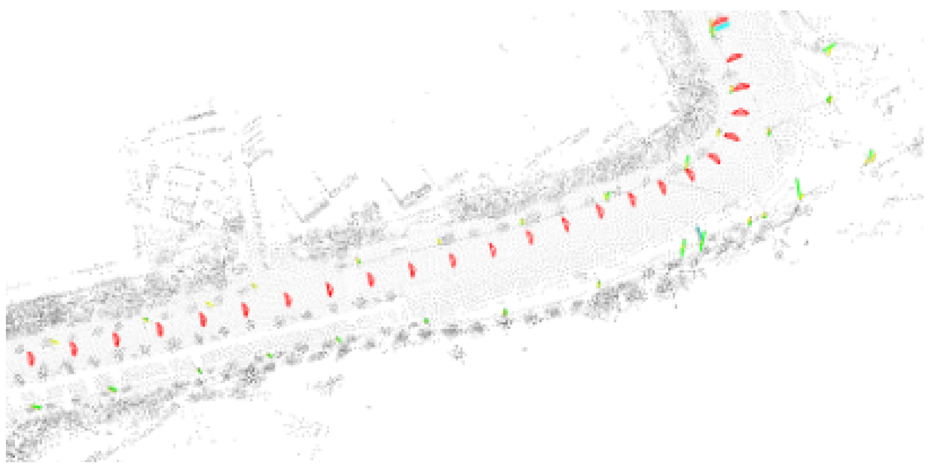
31] to ensure a more-accurate reconstruction of pole-like elements. The reconstruction result of this approach can be seen in Figure 5 where the poles along the linklet area of a vehicle are reconstructed.
Sign reconstruction: Here, we adopted the approach used in [31] to reconstruct the traffic sign by first estimating the plane model of the sign ( n , d ) . Then, the 3D position from the 2D contour points can be generated given that the depth λ of the control point { p i s } is solved with the condition of n T ( λ p i s ) = d , and its world coordinate can be obtained as:
λ = d n w · p i s , p w s = λ w R p i s + t
where x = { R , t } is the vehicle pose. We also used the rectangular and circular template points as our sign shape template as in [31]. The information for each reconstructed sign is saved as a set of points and the corresponding class of the sign, M w s = { p w s , C } . This information will be used in the next step to determine changes in the map.

3.4. Map Matching

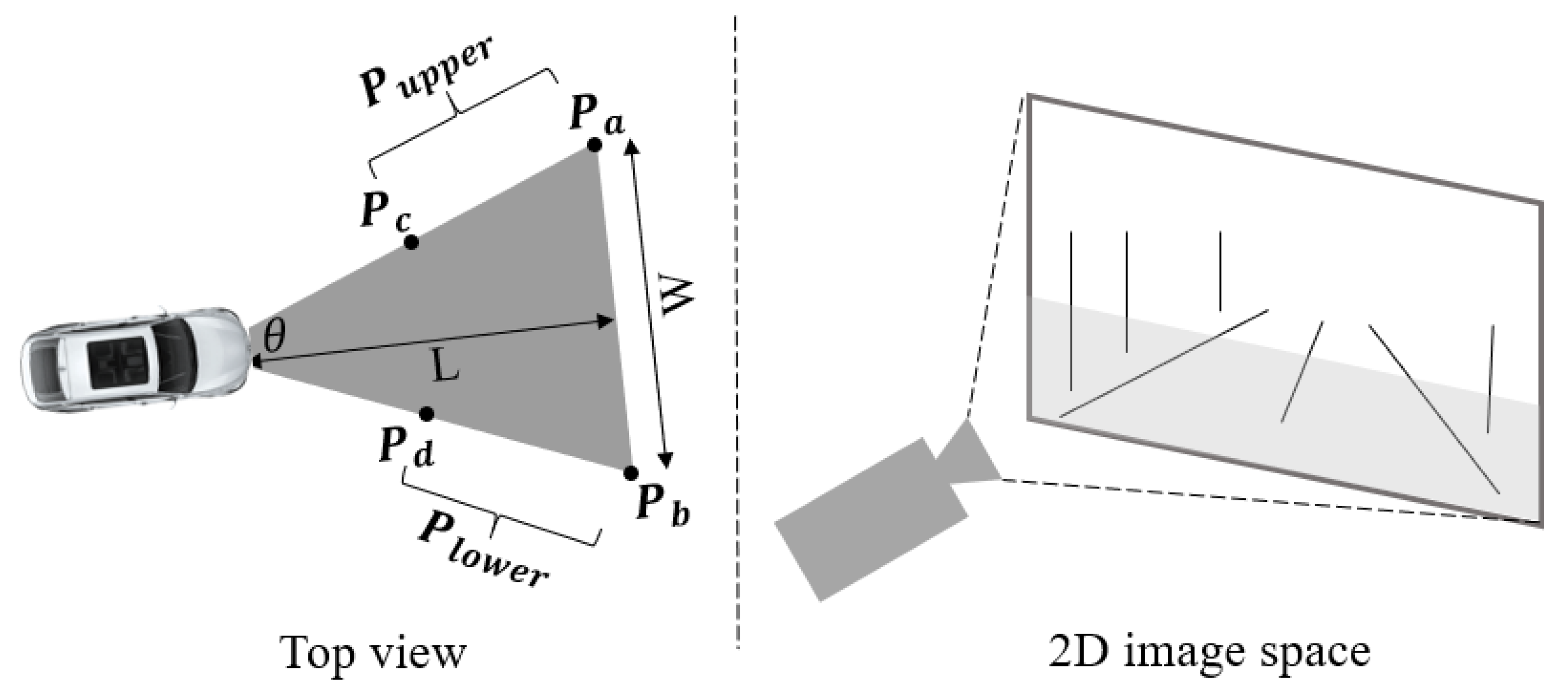
We propose an expected observation area that a vehicle will pass through on its trajectory. As shown in Figure 6, we define this area as an isosceles triangle with angle θ , length L, and width W. Then, the points P a and P b in the world coordinate can be obtained. It is important to note that the matching in this process is performed in the world coordinates. As the vehicle drives through its trajectory, the points P a and P b will create the expected observation area. This area is important for the vehicle to determine the limit of its observation since it is unrealistic to expect a vehicle to be able to have a full observation of all map elements that it passes through. The limit can be defined by two sets of points P u p p e r = { P c t = 1 , P a t = 1 , P a t = 2 , , P a t = T } and P l o w e r = { P d t = 1 , P b t = 1 , P b t = 2 , , P b t = T } .
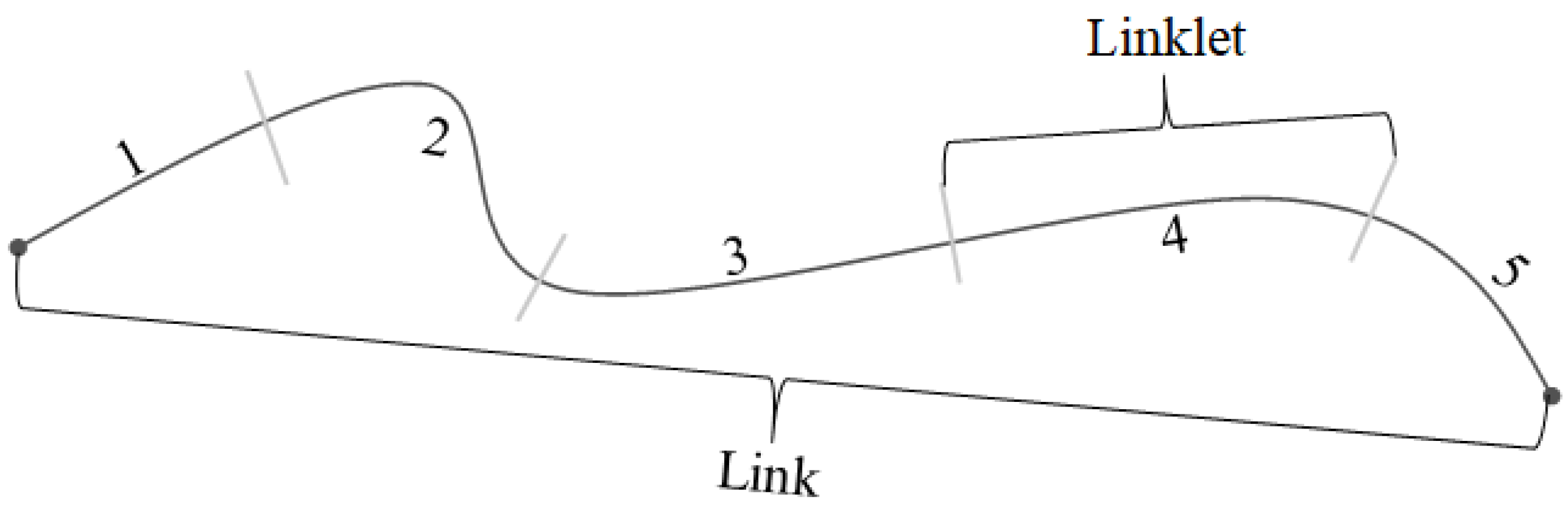
Through this model, we can determine the unmatched map elements to be out of limit or the map element to no longer exist. Here, we denote the map elements that belong to the expected observation inside the linklet area e as M e L M a l l L . The map elements that belong to M e L satisfy the constraint as shown below:
arg min t ( M e L P u p p e r t + M e L P l o w e r t ) W + Th
After we are able to find the map element sets that belong to the expected observation area, we can then match them with the list of detected map elements M w s , p , l . The matching process is performed via a point-based approach to simplify the calculation on the vehicle side. Given that all the lane line point sets from the map database are D l = { M 1 l , , M a l } , the poles sets from the map database are D p = { M 1 p , , M b p } , the sign sets from the map database are D s = { M 1 s , , M c s } , the lane line detection points in the 3D world coordinate are R l = { p 1 l , , p i l } , the pole points are R p = { p 1 p , , p j p } , and the sign points are R s = { p 1 s , , p k s } , then the map database set can be defined as: M e L = { ( M e l , M e p , M e s ) : M e l D l , M e p D p , M e s D s } and the map element detection set can be defined as M w = { ( M w l , M w p , M w s ) : M w l R l , M w p R p , M w s R s } . The distance matching is performed by considering only the detection result.
M m i , j L = 1 , arg min i , j { M e L M w } Th { l , p , s } 0 , arg min i , j { M e L M w } > Th { l , p , s }
Mm L = i , j M m i , j L
Thus, we can obtain the three important parameters, which are: map elements from the map database on the expected observation area M e L , map elements observed M w , and map elements matched Mm L . All of this information will be sent to the server as a result of single-session monitoring.

4. Multi-Session Monitoring

This section describes the server-side model and the back-end workflow for a multi-session monitoring framework. It uses the vehicles’ past locations and is based on a reporting system from the vehicle side that will be transferred to the server side. The absolute decision to decide whether the map has been changed or not should be based on multi-session map monitoring since it is richer in information.

4.1. Linklet Association

Following the approach of partitioning the map into several linklet areas by Pannen et al. [16], we are able to deploy our method for a large-scale map. We first created a cluster of vehicles passing each of the linklet areas to collect the vehicle data according to the trajectory taken by each vehicle. The visualization of the linklets’ area can be seen in Figure 7. In this process, we denote that, for each linklet L , the linklet transversal sets are T L = { T 1 L , , T W L } . For each transversal, we can receive information of the three parameters T n L = { ( M e L , M w , Mm L ) , n W } .

4.2. Monitoring Protocol

For the monitoring protocol, we are required to determine which linklet area has experienced a change based on the report from each vehicle. Given that the map has a number of linklets, we need to look for the linklet that has experienced the most change according to the vehicles passing through that area.
The urgency model as shown in Algorithm 1 above starts by combining the relative change experienced by each of the map elements Δ O E according to all the vehicles associated inside the linklet area T n L . This process can only be performed once the number of associated vehicles exceeds the threshold value of N T h . Then, we combine all of the change experienced by each map element by their weighted value λ E to calculate the linklet change value C L . When Δ O E exceeds the threshold value of the change C T h , the update urgency of the linklet area Z L changes to 1. The linklet change value is appended to the update urgency list C i u . The maximum value obtained from this list will point out the linklet area that most urgently requires an update.
Algorithm 1: Multi-session monitoring protocol.
Ijgi 13 00006 i001

5. Experimental Result

5.1. Experimental Setup

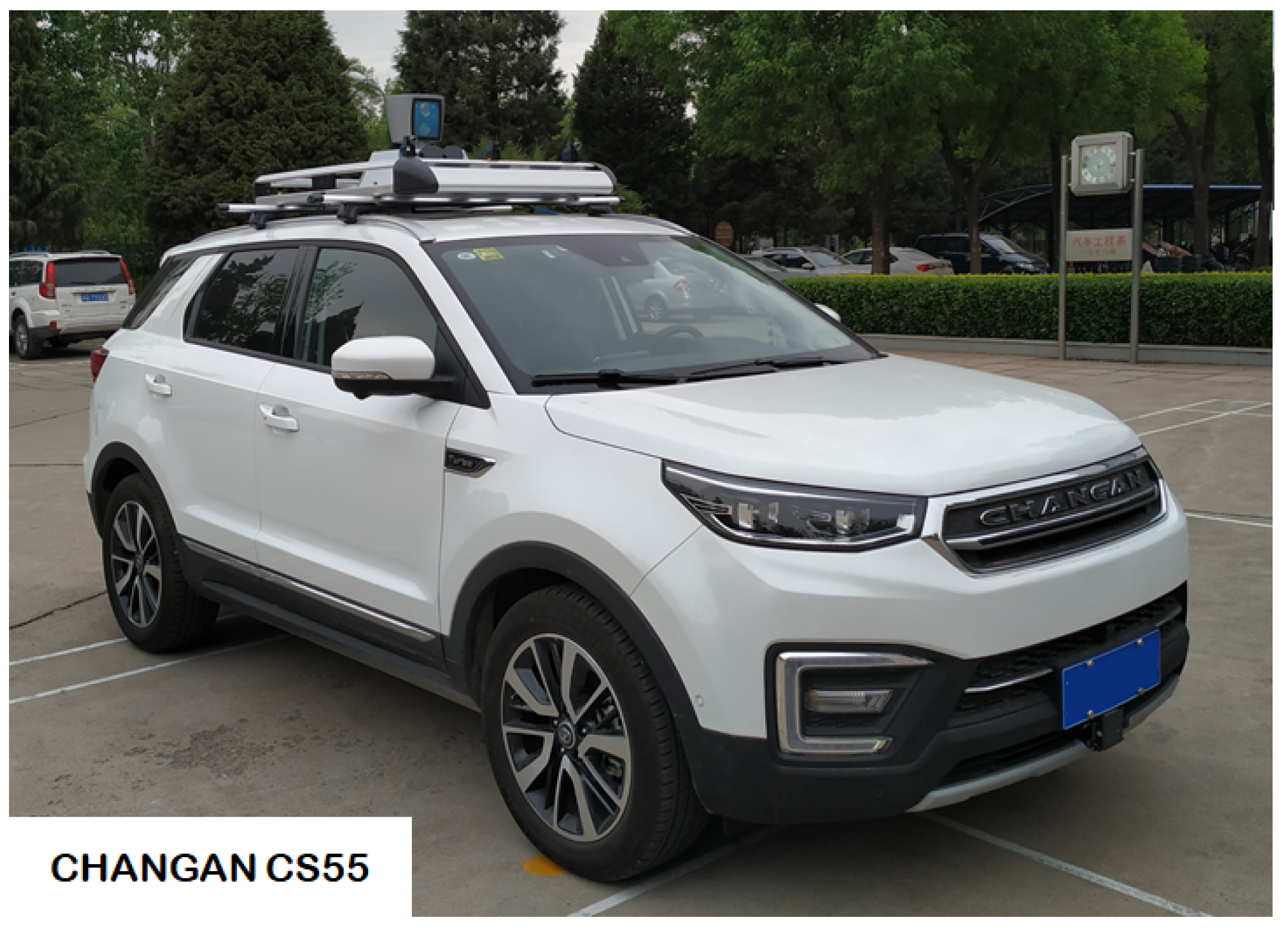
We simulated multi-session monitoring by traversing across Beijing Yizhuang District multiple times. Each time, the distance traveled was between 10 and 20 km. Therefore, several linklet areas were passed by the vehicle. Our experimental vehicle was equipped with a monocular camera with 1080p resolution recording at 10 fps. We also equipped the vehicle with an IMU sensor, gyroscope, and wheel encoder at 100 Hz. Although the vehicle was equipped with a Hesai 40P LiDAR sensor, the main localization tool used was GNSS-RTK to obtain high-precision positioning. The vehicle’s sensor details can be seen in Table 1, and the vehicle itself can be seen in Figure 8.
The whole Yizhuang District area was divided into 106 linklet areas, and we collected 20 sequences of data in this area, which will henceforth be referred to as the Yizhuang dataset. The data consisted of raw images and GNSS data complete with the timestamp information, and they will be used to evaluate the performance of our proposed method. To find the change on the map, we first removed some of the map data randomly to check whether our system is able to effectively and accurately detect the linklet areas that have this error. Furthermore, we checked the reconstruction results to further validate the map’s changes.

5.2. Evaluation Metric

In order to measure the accuracy of the multi-session monitoring system, we used the sensitivity (true positive rate (TPR) ) and specificity (true negative rate (TNR)) metrics from the confusion matrix that we generated.
T P R = T P ( T P + F N )
T N R = T N ( F P + T N )
where TPR is the true positive rate, TP is the true positive value, FN is the false negative value, TNR is the true negative rate, TN is the true negative value, and FP is the false positive value.
The TP and TN values give rise to the correct prediction as to whether or not there has been a change in the map, while the FP and FN values result in the wrong prediction. We determined the TP when our reconstructed data were different from the modified map data and matched the changes we previously made to the original map. This indicates that our monitoring algorithm has successfully detected the change. Conversely, we identified the FN when our reconstructed data matched the modified map data, despite there being a real-world change. For example, if there is a pole in reality and we have removed it from our data, but our reconstructed data also do not show the pole, this aligns with the modified map. This suggests that our algorithm incorrectly perceives no change, hence a false negative.

5.3. Monitoring Accuracy

Out of 106 linklet areas, we changed 40 linklet areas by either removing or shifting the map element in the world coordinate. It is important to note that, in these 40 linklet areas, we randomly changed the lane lines’, poles’, and traffic signs’ data. This process induced map error into the dataset. Here, we validate the result of our monitoring system through the detection of these changes in the map data, and the visualization of this map can be seen in Figure 9. We provide two types of monitoring accuracy: map-element-specific monitoring accuracy and linklet monitoring accuracy. The first accuracy determines the elementwise specificity of our change detection. The second accuracy provides us with a bigger picture of the overall result of our system.

5.3.1. Map-Element-Specific Monitoring Accuracy

In this subsection, we want to analyze the specificity of our monitoring algorithm. Figure 10 shows the amount of observations for each constructed map element in each of the linklet areas. It can be seen that there are some linklets that have no observations whatsoever, which is because not all the linklet areas are being passed by the vehicle. Here, we can see that, in most cases, the value of the ground truth and that of the reconstructed map element do not differ much. The association value is also close to the value of the changed map, which indicates that our method was able to find the change in the linklet. Given that we can observe most of the information the map provides to the vehicle, yet the vehicle is able to reconstruct additional details, this implies that the map lacks sufficient information, hinting at a need for updates or changes.
Additionally, we discovered that the ground truth map data were occasionally incomplete for certain objects like signs and poles. Take, for instance, the data for signs; the map only accounted for rectangular signs, which suggests a need for map updates. This issue is illustrated in Figure 11, where our system’s ability to identify such map inaccuracies is evident. However, to maintain the accuracy of our experiment, we excluded these instances from our analysis, as including erroneous ground truth data would significantly skew the accuracy of our method.

5.3.2. Linklet Monitoring Accuracy

After determining the map-element-specific changes, we can calculate the accuracy of our overall system by finding the changes we have created. As we can see in Table 2, our system managed to find 26 of the 27 changes that were made. For the remaining 35 linklet areas that had not experienced changes, our system gave the correct decision for 31 of them. Overall, we were able to achieve above 90% accuracy in the TPR and TNR.
The cases where our system detected false changes were mostly caused by the topology problem of the lane lines. The ID assignment of the reconstructed lane lines did not match the ID from the map data, thus causing the system to think that there was a change on the map because of a lack of the amount of matched IDs. However, after manually determining the starting and ending of the lane lines, the impact of the problem could be minimized.

5.4. Time Efficiency

To evaluate the runtime performance of the proposed algorithm, the single-session system was tested on an i7-6700 CPU and NVIDIA Quadro V100 GPU. The GPU was mainly used in the map element detection and object tracking part, and then, the CPU was used for the rest of the system. The multi-session system was tested on an i7-9850H CPU for all the modules. However, it is important to note that we did not consider the cost of information transmission since it is heavily dependent on the signal coverage of the area. That being said, considering the type of information and the size of it, which was about 8 to 14 KB/image, we can safely assume that the runtime will be very quick in normal circumstances. The average processing time can be seen in Table 3.
From the timing data, we can learn that the processing bottlenecks are in the machine learning estimation because of the neural network computation. The rest of the algorithms are considered lightweight compared to these two modules. This result demonstrated that our system is efficient in terms of computational requirements.

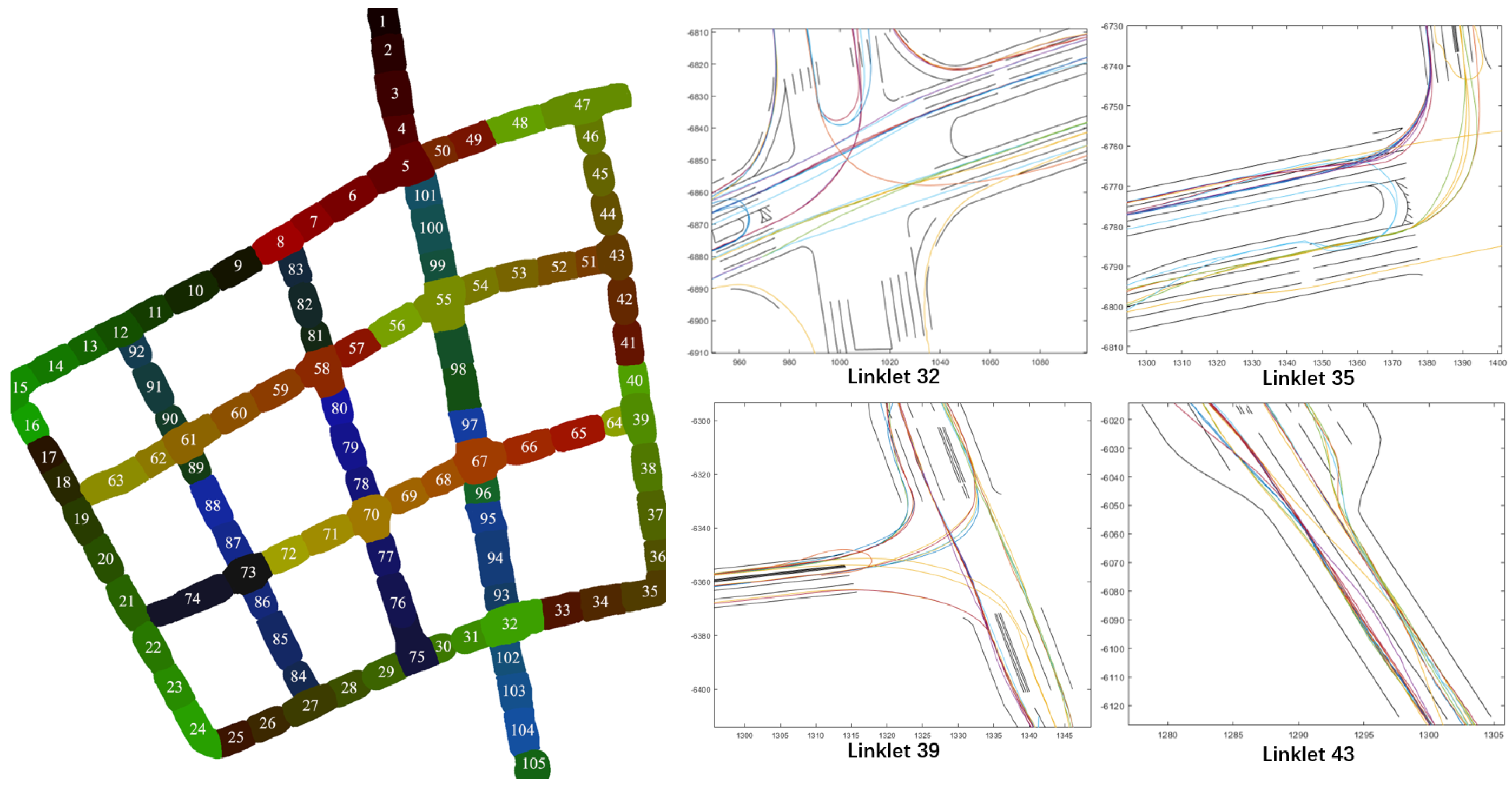
5.5. Challenging Cases

As shown in 
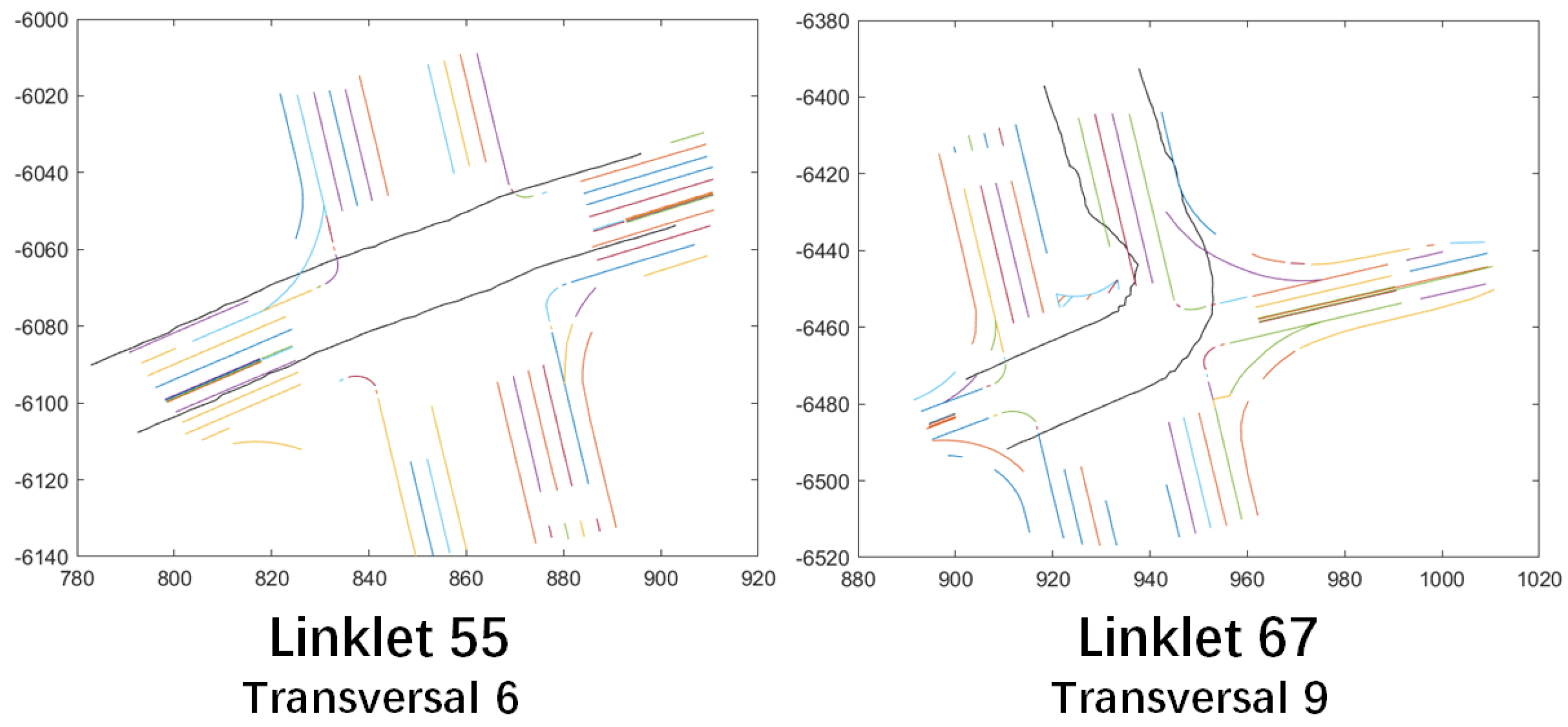
Figure 12, we found that the most-challenging cases within this experiment were mostly the division of the lane line IDs of the map at road intersection areas, where a higher number of lane lines can be found. Here, the different lane line colors represent different lane line IDs. This problem directly correlates with how the topology of the lanes is defined, and it might differ from the topology definition of the reconstruction result. This problem increases the value of the change even though there is little to no change in the map. Therefore, we performed manual adjustments of the lane topology in the local map. It is important to optimize this problem in the future to automate the whole process.

6. Conclusions and Future Works

In this paper, we proposed a multi-session HD map-monitoring framework. By leveraging confidence detection obtained from a machine learning algorithm applied to each frame, we successfully performed tracking to compound these detections into a belief system of map element existence. We effectively monitored the map data through local map reconstruction and matching techniques. Additionally, we proposed the concept of an expected observation area, which restricted the region that the vehicle can observe, thereby ensuring the reliability of information on the reconstructed map. The viability of our method was demonstrated through real-experimental data, providing strong evidence of its effectiveness and potential for practical implementation. Moving forward, we will aim to expand the scope of our work by incorporating more map elements and more semantic information. We also will address the lane topology problem to ensure the efficiency of the map-monitoring performance, thereby enhancing the comprehensiveness and usefulness of HD map monitoring.

Author Contributions

Conceptualization, Benny Wijaya; Formal Analysis, Benny Wijaya and Yunlong Wang; Methodology, Tuopu Wen; Software, Benny Wijaya; Validation, Benny Wijaya; Methodology, Benny Wijaya; Investigation, Zheng Fu, Xuewei Tang and Yunlong Wang; Resources, Mengmeng Yang, Kun Jiang and Diange Yang; Writing—original draft, Benny Wijaya, Jinyu Miaoand and Tuopu Wen; Writing—review & editing, Zheng Fu and Dennis Octovan Sigomo; Visualization, Xuewei Tang; Project administration, Tuopu Wen and Kun Jiang; Funding acquisition, Diange Yang and Mengmeng Yang; Supervision, Mengmeng Yang and Kun Jiang; All authors have read and agreed to the published version of the manuscript.

Funding

National Natural Science Foundation of China (52102464, U22A20104), PUSLAPDIK and LPDP.

Data Availability Statement

The data presented in this study are available on request from the corresponding author. The data are not publicly available due to privacy issue.

Conflicts of Interest

The authors declare no conflict of interest.

References

  1. SAE International. Taxonomy and Definitions for Terms Related to Driving Automation Systems for On-Road Motor Vehicles; SAE International: Warrendale, PA, USA, 2018; Volume 4970, pp. 1–5. [Google Scholar]
  2. Yang, D.G.; Jiang, K.; Zhao, D.; Yu, C.L.; Cao, Z.; Xie, S.C.; Xiao, Z.Y.; Jiao, X.Y.; Wang, S.J.; Zhang, K. Intelligent and connected vehicles: Current status and future perspectives. Sci. China Technol. Sci. 2018, 61, 1446–1471. [Google Scholar] [CrossRef]
  3. Badue, C.; Guidolini, R.; Carneiro, R.V.; Azevedo, P.; Cardoso, V.B.; Forechi, A.; Jesus, L.; Berriel, R.; Paixão, T.M.; Mutz, F.; et al. Self-driving cars: A survey. Expert Syst. Appl. 2021, 165, 113816. [Google Scholar] [CrossRef]
  4. Liu, Y.; Song, M.; Guo, Y. An incremental fusing method for high-definition map updating. In Proceedings of the IEEE International Conference on Systems, Man and Cybernetics, Bari, Italy, 6–9 October 2019; pp. 4251–4256. [Google Scholar] [CrossRef]
  5. AECC. Operational Behavior of a High Definition Map Application White Paper; AECC: Melbourne, Australia, 2020. [Google Scholar]
  6. Yang, B.; Liang, M.; Urtasun, R. HDNET: Exploiting HD maps for 3D object detection. arXiv 2020, arXiv:2012.11704. [Google Scholar]
  7. Ma, W.C.; Urtasun, R.; Tartavull, I.; Barsan, I.A.; Wang, S.; Bai, M.; Mattyus, G.; Homayounfar, N.; Lakshmikanth, S.K.; Pokrovsky, A. Exploiting Sparse Semantic HD Maps for Self-Driving Vehicle Localization. In Proceedings of the IEEE International Conference on Intelligent Robots and Systems, Macau, China, 3–8 November 2019; pp. 5304–5311. [Google Scholar] [CrossRef]
  8. Mattyus, G.; Wang, S.; Fidler, S.; Urtasun, R. HD Maps: Fine-Grained Road Segmentation by Parsing Ground and Aerial Images. In Proceedings of the IEEE Computer Society Conference on Computer Vision and Pattern Recognition, Las Vegas, NV, USA, 27–30 June 2016; pp. 3611–3619. [Google Scholar] [CrossRef]
  9. Mi, L.; Zhao, H.; Nash, C.; Jin, X.; Gao, J.; Sun, C.; Schmid, C.; Shavit, N.; Chai, Y.; Anguelov, D. HDMapGen: A Hierarchical Graph Generative Model of High Definition Maps. In Proceedings of the IEEE Computer Society Conference on Computer Vision and Pattern Recognition, Nashville, TN, USA, 20–25 June 2021; pp. 4225–4234. [Google Scholar] [CrossRef]
  10. Das, A.; Ijsselmuiden, J.; Dubbelman, G. Pose-graph based crowdsourced mapping framework. In Proceedings of the 2020 IEEE 3rd Connected and Automated Vehicles Symposium, CAVS, Victoria, BC, Canada, 18 November–16 December 2020. [Google Scholar] [CrossRef]
  11. Wong, K.; Gu, Y.; Kamijo, S. Mapping for autonomous driving: Opportunities and challenges. IEEE Intell. Transp. Syst. Mag. 2021, 13, 91–106. [Google Scholar] [CrossRef]
  12. Stoven-Dubois, A.; Miguel, K.K.; Dziri, A.; Leroy, B.; Chapuis, R. A Collaborative Framework for High-Definition Mapping. In Proceedings of the IEEE Intelligent Transportation Systems Conference, ITSC, Auckland, New Zealand, 27–30 October 2019; pp. 1845–1850. [Google Scholar] [CrossRef]
  13. Bao, Z.; Hossain, S.; Lang, H.; Lin, X. High-Definition Map Generation Technologies For Autonomous Driving. arXiv 2022, arXiv:2206.05400. [Google Scholar]
  14. Pannen, D.; Liebner, M.; Burgard, W. HD map change detection with a boosted particle filter. In Proceedings of the IEEE International Conference on Robotics and Automation, Montreal, QC, Canada, 20–24 May 2019; pp. 2561–2567. [Google Scholar] [CrossRef]
  15. Jo, K.; Kim, C.; Sunwoo, M. Simultaneous localization and map change update for the high definition map-based autonomous driving car. Sensors 2018, 18, 3145. [Google Scholar] [CrossRef] [PubMed]
  16. Pannen, D.; Liebner, M.; Hempel, W.; Burgard, W. How to Keep HD Maps for Automated Driving Up To Date. In Proceedings of the IEEE International Conference on Robotics and Automation, Paris, France, 31 May–31 August 2020; pp. 2288–2294. [Google Scholar]
  17. Heo, M.; Kim, J.; Kim, S. HD Map Change Detection with Cross-Domain Deep Metric Learning. In Proceedings of the 2020 IEEE/RSJ International Conference on Intelligent Robots and Systems (IROS), Las Vegas, NV, USA, 24 October–24 January 2021; pp. 10218–10224. [Google Scholar]
  18. Wijaya, B.; Jiang, K.; Yang, M.; Wen, T.; Tang, X.; Yang, D.; Ma, Y.; Albert, R. CrowdRep: A Blockchain-based Reputation System for Crowdsourced HD Map Update. In Proceedings of the IEEE Conference on Intelligent Transportation Systems, Proceedings, ITSC, Macau, China, 8–12 October 2022; pp. 3050–3057. [Google Scholar] [CrossRef]
  19. Liebner, M.; Jain, D.; Schauseil, J.; Pannen, D.; Hackeloer, A. Crowdsourced HD map patches based on road model inference and graph-based slam. In Proceedings of the IEEE Intelligent Vehicles Symposium, Macau, China, 8–12 October 2022; pp. 1211–1218. [Google Scholar] [CrossRef]
  20. Chao, P.; Hua, W.; Zhou, X. Trajectories know where map is wrong: An iterative framework for map-trajectory co-optimisation. World Wide Web 2020, 23, 47–73. [Google Scholar] [CrossRef]
  21. Cho, M.; Kim, K.; Cho, S.; Cho, S.M.; Chung, W. Frequent and Automatic Update of Lane-Level HD Maps with a Large Amount of Crowdsourced Data Acquired from Buses and Taxis in Seoul. Sensors 2023, 23, 438. [Google Scholar]
  22. Lambert, J.; Hays, J. Trust, but Verify: Cross-Modality Fusion for HD Map Change Detection. arXiv 2021, arXiv:2212.07312. [Google Scholar]
  23. Zhang, P.; Zhang, M.; Liu, J. Real-time hd map change detection for crowdsourcing update based on mid-to-high-end sensors. Sensors 2021, 21, 2477. [Google Scholar] [CrossRef]
  24. Fischler, M.A.; Bolles, R.C. Random Sample Paradigm for Model Consensus: A Apphcatlons to Image Fitting with Analysis and Automated Cartography. Graph. Image Process. 1981, 24, 381–395. [Google Scholar]
  25. Li, B.; Song, D.; Kingery, A.; Zheng, D.; Xu, Y.; Guo, H. Lane marking verification for high definition map maintenance using crowdsourced images. In Proceedings of the IEEE International Conference on Intelligent Robots and Systems, Las Vegas, NV, USA, 24 October–24 January 2020; pp. 2324–2329. [Google Scholar] [CrossRef]
  26. Kim, C.; Cho, S.; Sunwoo, M.; Resende, P.; Bradai, B.; Jo, K. Updating Point Cloud Layer of High Definition (HD) Map Based on Crowd-Sourcing of Multiple Vehicles Installed LiDAR. IEEE Access 2021, 9, 8028–8046. [Google Scholar] [CrossRef]
  27. He, K.; Gkioxari, G.; Dollár, P.; Girshick, R. Mask r-cnn. In Proceedings of the IEEE International Conference on Computer Vision, Venice, Italy, 22–29 October 2017; pp. 2961–2969. [Google Scholar]
  28. Neven, D.; De Brabandere, B.; Georgoulis, S.; Proesmans, M.; Van Gool, L. Towards End-to-End Lane Detection: An Instance Segmentation Approach. In Proceedings of the IEEE Intelligent Vehicles Symposium, Changshu, China, 26–30 June 2018; pp. 286–291. [Google Scholar] [CrossRef]
  29. Teed, Z.; Deng, J. Raft: Recurrent all-pairs field transforms for optical flow. In Proceedings of the European Conference on Computer Vision, Glasgow, UK, 23–28 August 2020; pp. 402–419. [Google Scholar]
  30. Brox, T.; Bruhn, A.; Papenberg, N.; Weickert, J. High Accuracy Optical Flow Estimation Based on a Theory for Warping. In Proceedings of the Computer Vision—ECCV 2004, Prague, Czech Republic, 11–14 May 2004; pp. 25–36. [Google Scholar]
  31. Wen, T.; Jiang, K.; Miao, J.; Wijaya, B.; Jia, P.; Yang, M.; Yang, D. Roadside HD Map Object Reconstruction Using Monocular Camera. IEEE Robot. Autom. Lett. 2022, 7, 7722–7729. [Google Scholar] [CrossRef]
Figure 1. Visualization of multi-session monitoring generated from detection confidence.
Ijgi 13 00006 g001
Figure 2. Multi-session map-monitoring framework from starting from a single session to determine the change in the HD map linklet area.
Ijgi 13 00006 g002
Figure 3. Tracking object limits for ground map element and vertical map elements.
Ijgi 13 00006 g003
Figure 4. Occupancy object template for map elements inside a continuous time series.
Ijgi 13 00006 g004
Figure 5. An illustration of the reconstruction of the pole-like elements of a local linklet area. The green color indicates the reconstructed poles and the red triangle indicates the vehicle’s pose.
Ijgi 13 00006 g005
Figure 6. The visualization of expected observation area.
Ijgi 13 00006 g006
Figure 7. The visualization of linklets’ area in high-definition map topology links.
Ijgi 13 00006 g007
Figure 8. The vehicle used to collect the data for this experiment is equipped with the GNSS-RTK, IMU, monocular camera, and LiDAR sensor.
Ijgi 13 00006 g008
Figure 9. The visualization of the scale of the map monitored in this experiment, where each unique color symbolizes a linklet area and the colorful lines on the right side denote the transversals that happen in each of the linklet areas.
Ijgi 13 00006 g009
Figure 10. The number of map elements monitored during the vehicle transversals inside the linklet area: (a) traffic signs; (b) poles; (c) lane lines.
Ijgi 13 00006 g010
Figure 11. The visualization of the map projection in black and map element detection in green.
Ijgi 13 00006 g011
Figure 12. The challenging cases where the lane line IDs inside the intersection area are higher compared to the lane line IDs reconstructed. The different line color indicates line ID, and the black line is the observation area of the vehicle.
Ijgi 13 00006 g012
Table 1. Sensors equipped on the vehicles.
Sensor TypeSensor NameSensor Configuration
CameraStereolabs ZED 21920 × 1080 @10 fps
LiDARHesai 40P LiDAR-
RTK-GNSS/IMUNovAtel PP7D-E1Acc. 10 cm @100 hz
GPS sensorUblox F9PAcc. 10 m @100 hz
Computational ModuleNuvo-6108GCIntel i7 + GTX 1080
Table 2. The map change detection accuracy of our multi-session monitoring system.
Linklet PassedCh. Linklet PassedLinklet Change DetectedMon. Accuracy
True Pos.False Pos.TPRTNR
622726392.86%91.17%
Table 3. Average time cost per image for single-session system and per monitoring cycle for multi-session system.
Main ModuleTime
Single-SessionMap element detection175 ms
Object tracking166.6 ms
Bayesian inference6.3 ms
Map reconstruction45.2 ms
Map matching12.5 ms
Multi-SessionLinklet association13.2 ms
Multi-vehicle change detection15.4 ms
Total time434.2 ms
Disclaimer/Publisher’s Note: The statements, opinions and data contained in all publications are solely those of the individual author(s) and contributor(s) and not of MDPI and/or the editor(s). MDPI and/or the editor(s) disclaim responsibility for any injury to people or property resulting from any ideas, methods, instructions or products referred to in the content.

