Article

Drainage Pattern Recognition of River Network Based on Graph Convolutional Neural Network

1
College of Urban and Environmental Sciences, Central China Normal University, Wuhan 430079, China
2
Wuhan Natural Resources and Planning Information Center, Wuhan 430014, China
3
Key Laboratory for Geographical Process Analysis & Simulation of Hubei Province, Wuhan 430079, China
4
Wuhan Geomatics Institute, Wuhan 430022, China
*
Author to whom correspondence should be addressed.
ISPRS Int. J. Geo-Inf. 2023, 12(7), 253; https://doi.org/10.3390/ijgi12070253
Submission received: 27 February 2023 / Revised: 15 June 2023 / Accepted: 16 June 2023 / Published: 21 June 2023

Abstract

:
Drainage network pattern recognition is a significant task with wide applications in geographic information mining, map cartography, water resources management, and urban planning. Accurate identification of spatial patterns in river networks can help us understand geographic phenomena, optimize map cartographic quality, assess water resource potential, and provide a scientific basis for urban development planning. However, river network pattern recognition still faces challenges due to the complexity and diversity of river networks. To address this issue, this study proposes a river network pattern recognition method based on graph convolutional networks (GCNs), aiming to achieve accurate classification of different river network patterns. We utilize binary trees to construct a hierarchical tree structure based on river reaches and progressively determine the tree hierarchy by identifying the upstream and downstream relationships among river reaches. Based on this representation, input features for the graph convolutional model are extracted from both spatial and geometric perspectives. The effectiveness of the proposed method is validated through classification experiments on four types of vector river network data (dendritic, fan-shaped, trellis, and fan-shaped). The experimental results demonstrate that the proposed method can effectively classify vector river networks, providing strong support for research and applications in related fields.

1. Introduction

River networks are vital components of the natural environment and play a crucial role as prominent geospatial features, often referred to as the “skeletal lines” of the terrain [1]. They are shaped and influenced by various factors such as local geology, climate conditions, and human interventions. Through the interaction of human activities and natural processes, distinct morphological characteristics gradually emerge within river networks in different regions. Concurrently, these characteristics reciprocally impact the evolution of both natural and cultural landscapes [2]. These traits manifest in the plan view of river networks, granting them distinguishable spatial patterns, commonly known as river network patterns. Automated detection and feature analysis of river network patterns find extensive applications in fields such as hydrology, geology, urban planning, floodplain mapping, etc. For instance, the classification of river network types assumes significance as a key parameter in hydrological frequency analysis. Furthermore, differentiating between river networks aids in identifying various network types and facilitates the comprehension of natural evolutionary processes. In the realm of map cartography, recognizing the spatial patterns of river networks serves as a preliminary step in comprehensive river network analysis. Proper synthesis strategies are chosen based on the spatial distribution patterns of river networks during the process of river network synthesis [3].
In GIS, drainage systems are typically digitized as polylines. So far, most research on organizing river network data has been based on the concept of river reaches [4,5,6,7,8,9]. River reaches, also referred to as links or segments, represent a section of a river between confluences or between a confluence and a source. A river network is composed of a collection of interconnected river reaches. Numerous researchers have quantitatively described the characteristics of river networks based on this representation [10,11,12,13] and subsequently attempted to achieve automatic identification of river network patterns based on their planar morphology [14,15,16]. Argialas et al. [11], Du et al. [14], Zhang and Guilbert [15], and others extracted geometric features of river networks and employed decision trees, an analytic hierarchy process, and fuzzy set theory to classify different river networks. Mejía and Niemann [17] identified river network types by analyzing their self-similarity. Jung et al. [16] utilized the beta distribution characteristics of confluence angles and support vector machines to classify certain drainage systems. Touya [3] even applied pattern recognition of drainage systems in the selection process of river network synthesis. Despite some achievements so far, automatic identification of river network patterns remains a complex task due to the diverse morphology and complex formation processes of natural networks such as river networks.
Most of the automatic identification methods for river network patterns introduced earlier are model-driven approaches, where researchers design different classification models based on their experience and train them with a small number of samples. Although these models can differentiate some typical cases, they still cannot fully meet the needs of recognizing complex geographical features such as river networks. In comparison to traditional model-driven methods, deep learning methods have the following advantages: (i) a strong representation capability, as deep learning models can learn abstract representations of input data through multi-level non-linear transformations, enabling them to capture richer and more complex features and patterns; and (ii) automatic feature learning, where deep learning can automatically learn task-specific feature representations from raw data, alleviating the burden of feature engineering. However, deep learning methods, such as convolutional neural networks (CNNs), are typically applied to raster-based spatial information [18,19,20]. Recently, there has been an emergence of graph convolutional neural networks (GCNs), a deep learning approach based on graph structures. This method is particularly suitable for handling spatial vector data and is considered a new direction in deep learning [21]. Geographic spatial vector data is a typical non-standardized data type that is often studied using graph theory methods. Therefore, applying graph convolutional neural networks to research related to geographic spatial data, represented by river networks, is a feasible solution.
Currently, some researchers have started to apply deep learning methods to the task of river network pattern recognition. Donadio et al. [22] initially used a CNN to identify dendritic and non-dendritic patterns. However, transforming structured vector data into sequentially ordered raster data disrupts the structural content of GIS graphic information and fails to effectively utilize the characteristics of vector data. Compared to CNNs that rely on image-based approaches for recognition, graph-based deep learning methods do not require the conversion between vector and raster data, making them more flexible and direct. This point has also been demonstrated in the study by Yu et al. [23].
This study proposes a river network pattern recognition method based on a GCN. We represent the river network using a binary tree structure and extract features from geometric and spatial perspectives. GCN and multilayer perceptron (MLP) are utilized for pattern classification and prediction. In the experiments, we validate the effectiveness of this method using cases of dendritic, trellis, comb, and fan-shaped drainage networks. Furthermore, we examine the impact of different feature combinations on the model’s classification ability. It is important to note that our sample selection does not entirely follow real river basins. Firstly, large river systems are typically composed of composite patterns formed by different types of sub-basins, and the ideal approach is to gradually classify large river systems with composite patterns into specific types [12]. However, there is currently no automatic method available for classifying complex drainage networks. Moreover, for the task of complex river network pattern recognition, we consider the recognition of basic river systems to be a more fundamental and important task. Secondly, although river networks are one of the most widespread elements in the natural world, the quantities of different types of river networks are uneven. For example, dendritic networks are the most common, while other types are rare in real river basins. Insufficient samples or imbalanced sample distribution of different types can lead to overfitting or under-sampling issues in deep learning methods. Finally, existing river network pattern recognition methods are mostly based on two-dimensional geometry [24]. These drainage networks possess typical characteristics, and by effectively utilizing different features of river networks as planar graphs, they can distinguish different types of river networks. Therefore, for the task of river network pattern recognition, we believe that apart from the regional context, there exist fundamental drainage network patterns and their derived patterns that occur repeatedly. When selecting samples, it is recommended to disregard the regional context and rely on empirical knowledge to choose a set of samples that align with common patterns based on their morphological characteristics.
The subsequent sections of the paper are organized as follows. Section 2 provides a detailed description of the model design and implementation based on graph convolutional networks. Section 3 presents the experimental evaluation of the model, including dataset partitioning, the training process, and classification results. Section 4 concludes the paper with a summary and discussion.

2. Method for Spatial Pattern Recognition Method for Drainage Networks

2.1. Framework of Drainage Network Pattern Recognition

The framework for drainage pattern recognition based on GCN consists of four components: constructing a sample library, formalizing the representation of drainage networks, extracting indicators to describe drainage networks, and building the model based on GCN for experimentation (Figure 1):
(1)
Constructing a sample library: Extracting vector river network data from DEM for experimental purposes.
(2)
Graph representation: Utilizing a binary tree structure (a specific type of graph) to construct the river network structure based on river reaches.
(3)
Indicator description: Selecting appropriate geometric and spatial indicators to describe the river network.
(4)
Pattern recognition: Building a suitable neural network classification model based on GCN and conducting classification experiments using the graph structure data obtained from the aforementioned steps.

2.2. Tree Model Construction of Drainage Network

River networks represented by dendritic patterns typically have two upstream river reaches and one downstream river reach at river confluences. Given this characteristic, we consider the structure of river networks to be idealized. We assume that the branching point of a river in the study represents the intersection of two upstream river reaches and one downstream river reach, with each river network having only one outlet (river mouth reach). In cases where the river network data do not meet these conditions, manual corrections are applied. This assumption has also been adopted in previous studies [25,26]. River reaches are the basic units of river networks. Therefore, in this paper, a river network data structure based on river reaches is designed. More specifically, under the idealized conditions, the river network is formalized using a binary tree structure. In this structure, each river reach is treated as a node in the binary tree, and the connections between river reaches represent the edges between nodes. In the designed binary tree structure of the river network, the two converging upstream river reaches are the child nodes of the converging downstream river reach, and the corresponding downstream river reach is the parent node. The river mouth reach serves as the root node of the tree.
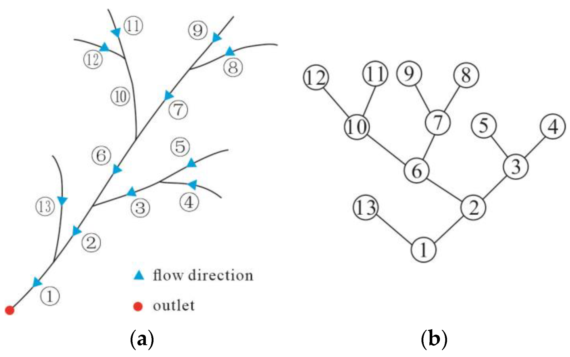
When constructing the binary tree structure of the river network, we start from the river mouth and trace upstream, progressively determining the tree structure of the river network following the pre-order traversal of the binary tree [27]. The resulting structure is the dual graph of the river network’s geometric pattern. Figure 2 provides an example of the structured river network, where the numbers indicate the order of accessing the river reaches.

2.3. Description Indices of Drainage Network

In this section, we will introduce the indices used to differentiate different types of drainage networks, which describe the river systems from both geometric and spatial perspectives. According to previous studies, confluence angles are important geometric features for distinguishing different river network patterns. In dendritic and fan-shaped networks, the confluence angles between river reaches are mostly acute, while in trellis and comb-shaped networks, the confluence angles tend to be close to right angles. In contrast to dendritic or fan-shaped networks, trellis and comb-shaped networks have shorter and straighter river reach lengths. Therefore, river reach length and sinuosity are used as indicators to differentiate these types. Unlike the other three network patterns, comb-shaped networks have their tributaries predominantly distributed on one side of the main channel, requiring the annotation of the positional relationship between adjacent river reaches for differentiation. Additionally, considering that these network types possess a hierarchical tree structure and exhibit significant differences, stream ordering is used as an index to differentiate river network categories.

2.3.1. Geometric Indices

(1) Length.
Length is a fundamental characteristic of linear features and one of the most commonly used indices. River reaches exhibit different length characteristics in various river networks. For example, in dendritic river networks, there is a significant variation in the lengths of rivers. Trellis and comb-like river networks, on the other hand, tend to have shorter lengths for their tributaries, while fan-shaped river networks can have varying lengths. However, the perception of “long” and “short” is relative in a geographical context, and it is not feasible to use absolute lengths of river reaches to distinguish different types of river networks. Therefore, an appropriate method is required to describe the length of river reaches. In this study, we employ normalization to represent the relative length of river reaches within their respective river networks. Specifically, we use min–max normalization, which maps the length of a river reach to the range of 0–1. The normalized length, denoted as xscale, is calculated as x scale = x x m i n x m a x x m i n , where x represents the length of the river reach, and xmax and xmin are the maximum and minimum lengths of the river network, respectively.
(2) Sinuosity.
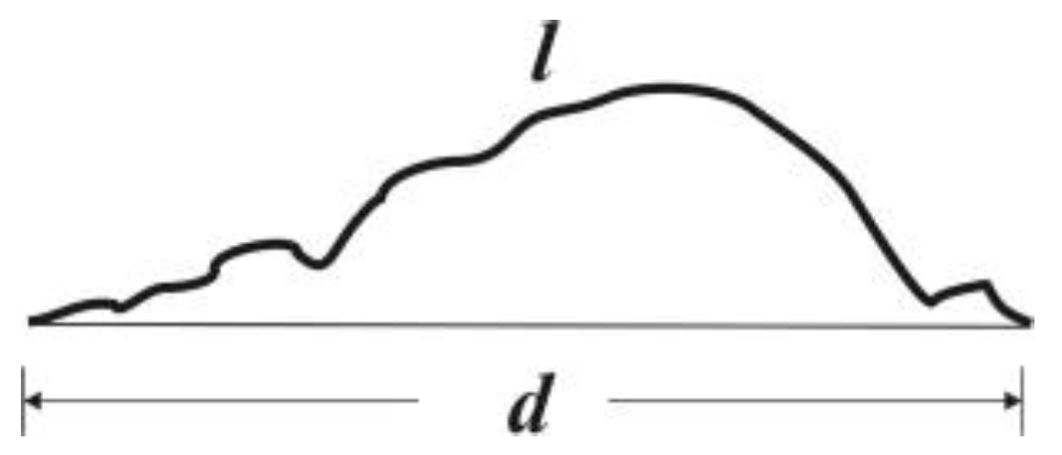
Rivers are formed within specific topographic environments, and the structured information encoded in their geographic features is primarily manifested through their curvature characteristics [28]. Existing studies have shown that the degree of meandering varies among different types of river networks. For example, rivers in trellis-like networks tend to be relatively straight, while those in fan-shaped networks exhibit greater meandering. The sinuosity of a river reach can be simply defined as the ratio of its length to the straight-line distance between its start and end points [14]. In Figure 3, l represents the actual length of a river reach, and d represents the straight-line distance between its start and end points.
(3) Confluence angle.
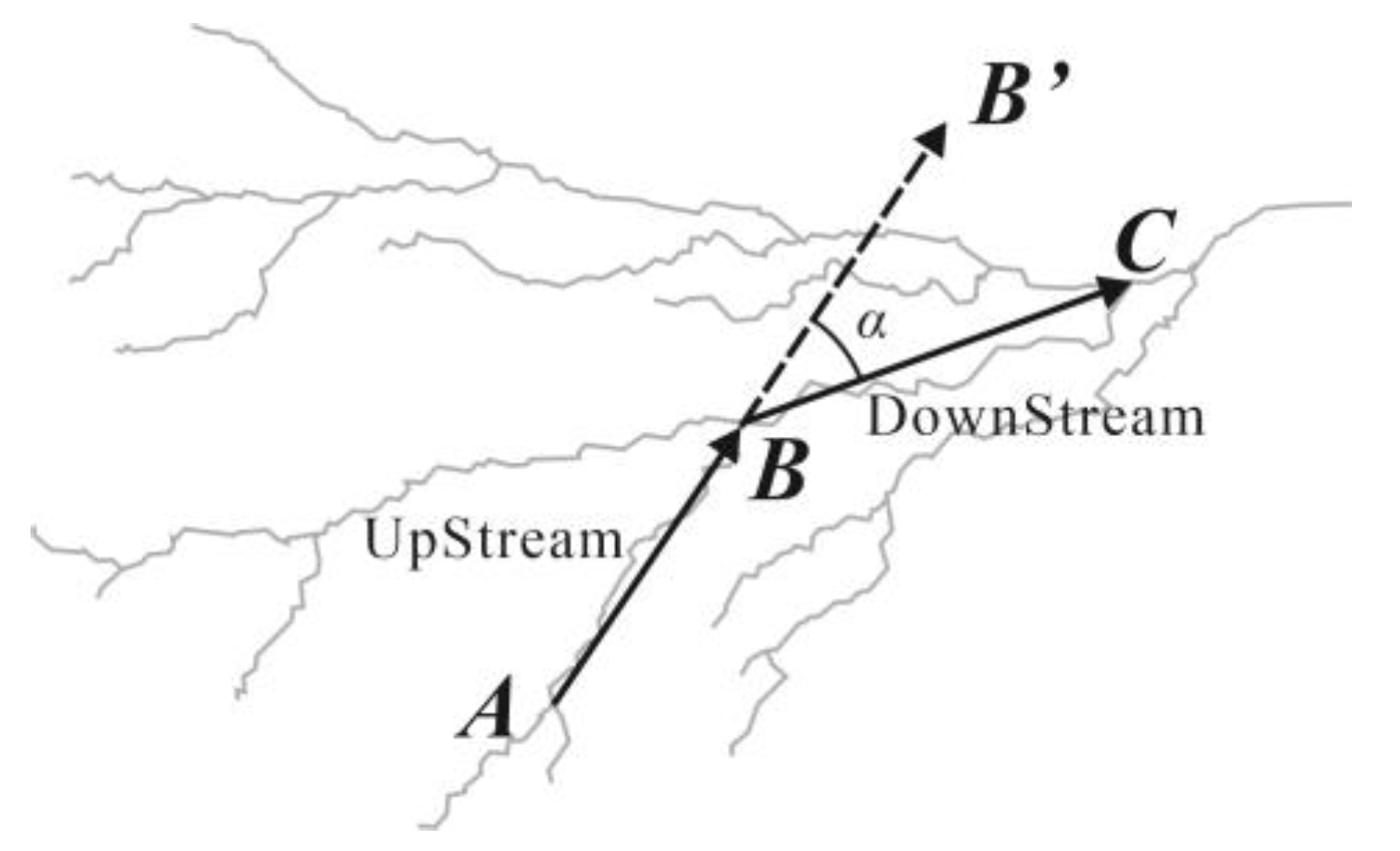
In contrast to some methods that calculate the upstream angle at confluences, the confluence angle used in this study refers to the angle between the upstream and downstream river reaches, without distinguishing between main stems and tributaries. For example, in Figure 4, river reaches AB and BC represent the upstream and downstream reaches, respectively, and the angle between them is denoted as α. The specific calculation method involves selecting three points on each of the two river reaches starting from the confluence and calculating the average angle between them. The confluence angle of a river ranges from 0° to 180°, and it is normalized using the equation x = θ 180 , where θ represents the angle value between river reaches, and x represents the normalized value.

2.3.2. Spatial Indices

(1) Left and right position identification.
This index is custom-defined based on the characteristics of the binary tree structure and the representation needs of the river network. Among the selected types of river networks, in a comb-like network, the tributaries are arranged in a parallel pattern on one side of the main stem, with similar orientations. In a trellis network, the tributaries are also arranged in a parallel pattern, but unlike the comb-like network, the tributaries are evenly distributed on both sides of the main stem. However, in a graph-based representation of the river network, it is not possible to solely determine the relative positions of the two upstream river reaches based on angles. Therefore, left and right positional indicators are used. In the actual calculation, the two intersecting upstream river reaches are represented by vectors. These vectors can be defined using the intersection point and the nearest point to it, with the direction representing the flow of water. The relative positions of the two vectors are determined by calculating the cross product of the two vectors and are indicated as 0 for the left position and 1 for the right position. The root node (river mouth) is identified as 0.
(2) Stream ordering.
The coding value of a river reach indicates its relative position within the entire river network and can also reflect the complexity of hierarchy within the network. The Strahler ordering [29] is employed for coding.

2.4. GCN Model for Drainage Network Pattern Recognition

GCNs are an extension of traditional deep learning methods for graph data, and they have shown remarkable performance in tasks related to irregular grid data. Similar to traditional deep learning methods, the learning process of GCNs can be viewed as learning graph features; for detailed principles, refer to the research by Kipf et al. [30]. Introducing the graph convolutional network approach enables the application of deep learning methods to irregular grid data such as river networks while preserving the topological structure, thereby facilitating pattern recognition.
After structural processing, a river network can be represented as G = V , E , where v V represents the river reaches in the network, and e E represents the connections between river reaches. The features of nodes or edges are embedded into the graph structure, where the feature matrix of nodes is denoted as X n × d , with n being the number of nodes and d being the dimensionality of node features. The edge feature, which is the convergence angle, is represented as a substitute value of 1 in the adjacency matrix A.
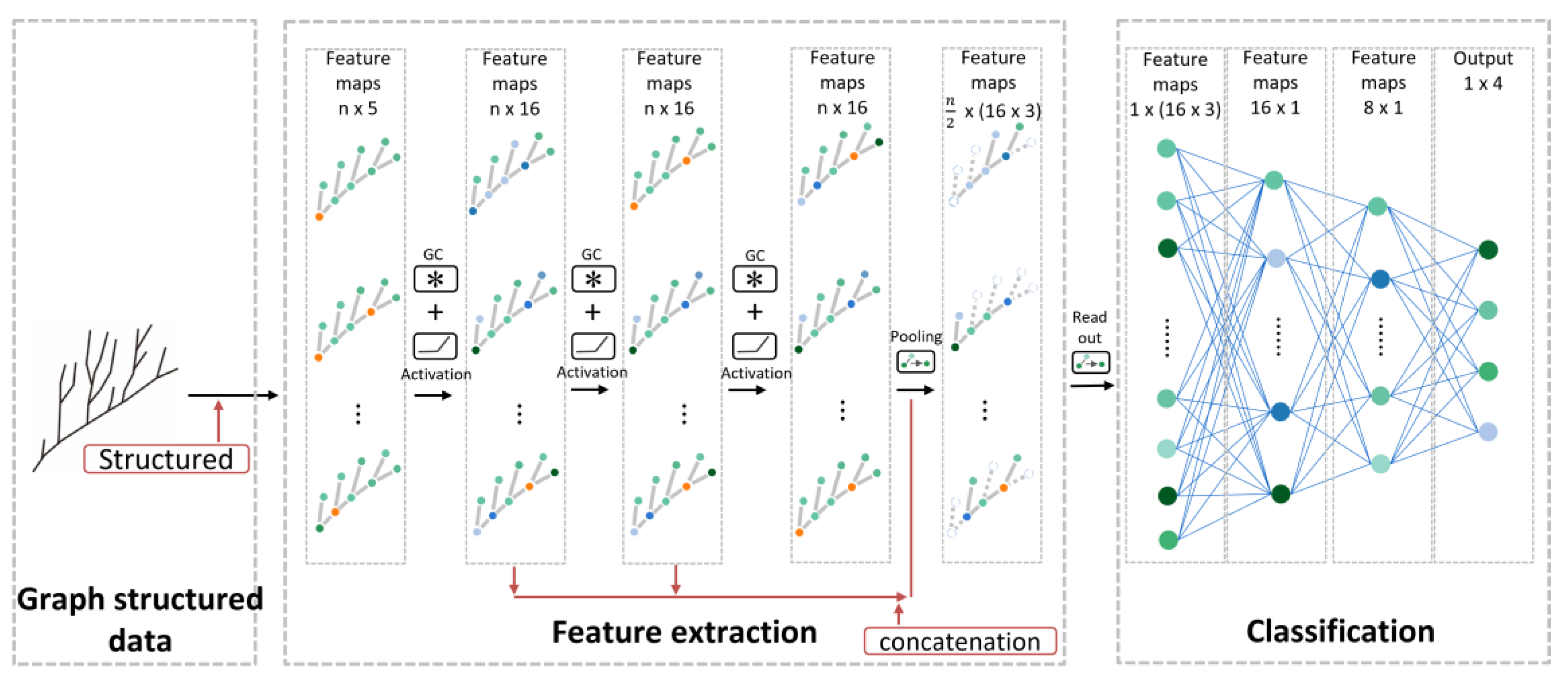
The river network classification model involved in this work mainly consists of structured river network, feature extraction, and classification network. The classification network used in the study includes a typical three-tier architecture: input layer (graph representation of the river network), hidden layers (3 graph convolutional layers, 2 graph pooling layers, 3 fully connected layers), and output layer (pattern recognition results). The network architecture we designed is shown in Figure 5. The forward propagation process in this network is as follows: given a drainage system graph G and the embedded water system feature vector X n × d , the input G is processed through graph convolution and pooling operations in the hidden layers to obtain the graph-level representation of the drainage system. Then, through the operations of the fully connected layers, the probability distribution at the graph level is obtained.
The stacked graph convolutional operations in the hidden layers optimize node features without altering the graph structure. After the graph convolution operation, each node is represented by a new feature, similar to the process of obtaining feature maps through convolution in CNNs. The operation of a graph convolutional layer can be described using a non-linear function: H l + 1 = f ( H l , A ) , where H l represents the input values of the l t h layer of the neural network, with H 0 = X n × d being the input layer. The graph convolution operation employs the graph convolution operator proposed by Kipf et al. [30], which is widely used in various tasks of graph convolutional networks. It can be specifically described as f ( H l , A ) = σ D ~ 1 2 A ~ D ~ 1 2 H l W l . Here, σ · denotes a non-linear activation function, and in this study, we use the ReLU function. D ~ 1 2 A ~ D ~ 1 2 represents the normalized Laplacian matrix of the graph, where D ~ is the diagonal matrix. W l represents the weight matrix for the l t h layer.
For node-level tasks, graph convolution operations are sufficient. However, river network pattern recognition involves graph-level classification tasks, and the number of nodes in different river network graphs may vary. Therefore, after the graph convolution operation, graph pooling is required. Graph pooling aggregates node features to generate features for the entire graph. In this study, we employ self-attention pooling (SAGPooling) for the pooling operation. This method learns the importance of nodes from the graph through graph convolution operations. Compared to other graph pooling methods, SAGPooling has the advantages of considering both node features and graph topology, as well as having reasonable complexity [31]. The core of SAGPooling is to use GCN to obtain scores for nodes, which represent their importance. The scores are computed as follows: Z = σ D ~ 1 2 A ~ D ~ 1 2 X W , where the parameters have the same meaning as those in the graph convolutional layer in the hidden layers.

3. Experiments and Results

In this section, we conducted experimental evaluations of the proposed pattern recognition model. The model was implemented using PyTorch Geometric (PyG) [32], which is one of the popular graph deep learning libraries. PyG was developed by Dr. Matthias Fey from the Technical University of Dortmund, based on the deep learning framework PyTorch. It allows for direct application on non-conventional data structures represented by graphs.

3.1. Data Description

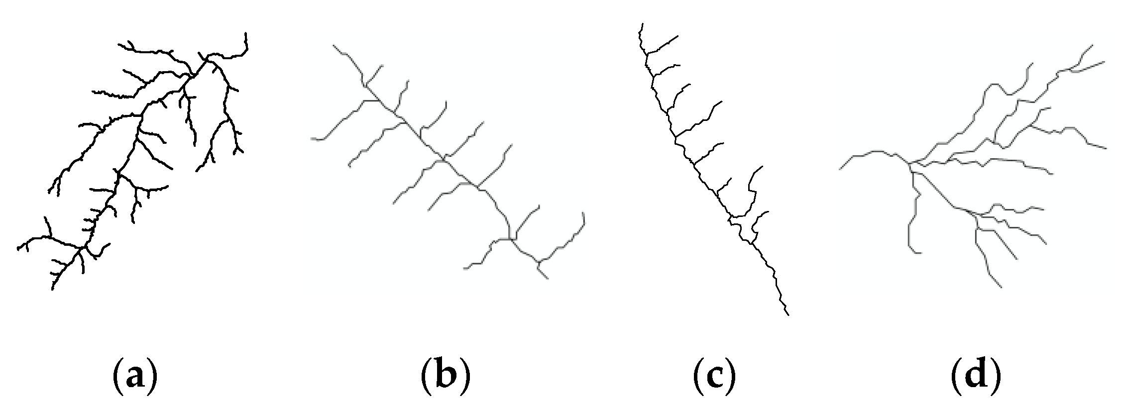
In this study, four types of river networks were included: dendritic, trellis, comb-like, and fan-shaped. Partial samples are shown in Figure 6. A total of 2000 river network samples were selected, with 500 samples for each type. The data were split into a training set and a test set in a 7:3 ratio, and 400 samples (100 for each type) were randomly chosen as the validation set.
The training and validation samples were selected from the GDEM-V2 dataset, a digital elevation model (DEM) with a spatial resolution of 30 m. The DEM data cover regions in China, including Hubei, Henan, Shaanxi, and Yunnan. The river networks were extracted from the DEM data. All rivers have a unique and well-defined flow direction, representing single-threaded rivers.
It is worth noting that the sample selection process did not strictly adhere to real-world river basins. Instead, a batch of samples with morphological features matching common patterns was selected based on experience to increase the sample quantity. Additionally, to avoid ambiguous drainage system patterns in the training set, sample selection was conducted by three GIS experts. Only samples that were unanimously agreed upon by all three participants as conforming to specific patterns were considered valid.
Statistically, dendritic river systems contain approximately 40 to 140 reaches per sample, while the other three types contain approximately 15 to 67 reaches per system. In total, the dataset includes 54,928 river reaches. The selected samples exhibit a branching ratio between 3 and 5, and a length ratio between 1.5 and 3.5, complying with Horton’s laws regarding the number of rivers and their lengths [33].

3.2. Drainage Network Classification Experiment

The classification experiment utilized a binary-tree-based construction of the graph structure based on reaches. The attributes of the graph nodes and edges are detailed in Table 1, where the descriptive feature parameters for the graph nodes consist of four variables, and the descriptive feature parameter for the edges consists of one variable. The model employed the ReLU function as the activation function. The model training followed a gradient descent approach guided by backpropagation, utilizing cross-entropy error as the loss function. The Adam optimization algorithm was used for gradient descent to optimize the model parameters. To prevent overfitting, a dropout layer was introduced after the first fully connected layer with a dropout rate of 50%. The other hyperparameters of the model, including the learning rate, L2 weight decay coefficient, and mini-batch size, were set to 0.01, 0.0001, and 128, respectively.
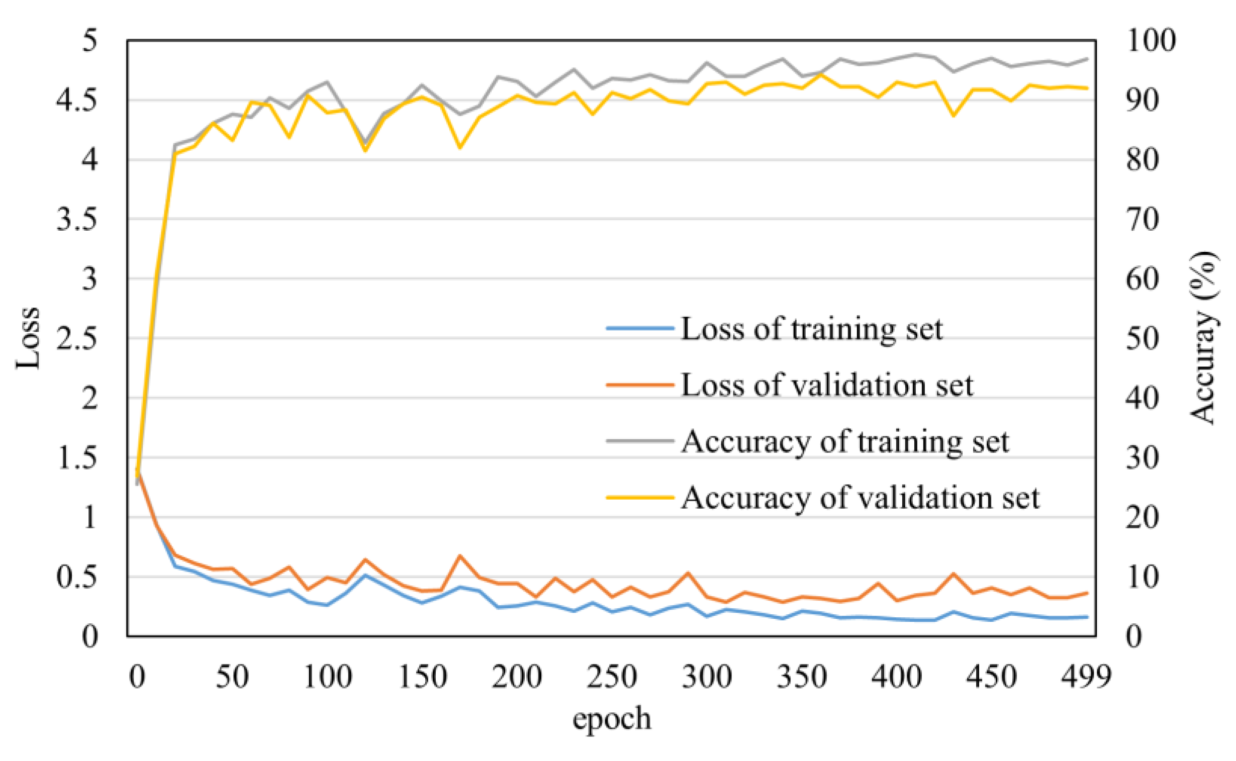
Figure 7 illustrates the accuracy changes of the training and validation sets during model training. As the number of training iterations increases, the predictive accuracy on the test set gradually improves, and after approximately 50 iterations, the accuracy on the validation set stabilizes. To prevent overfitting, if the loss value on the validation set does not decrease for consecutive 50 iterations during training, it is considered that the model has been sufficiently trained. At this point, the network training is terminated early, and the model parameters corresponding to the highest accuracy on the validation set are saved as the training result.
The model achieved a classification accuracy of 95.5% on the test set. Table 2 presents the confusion matrix of the model’s classification results on the test set. The values on the main diagonal of the confusion matrix represent the number of correctly classified instances for each class. The results indicate that the classification performance is highest for the dendritic river networks, with a 100% accuracy. The “comb-like” river networks follow with a 98% accuracy. The trellis and fan-shaped river networks achieved accuracies of 88% and 96%, respectively. Table 3 displays the experimental results for selected samples, where incorrectly classified samples are marked with F.
To provide a better explanation of the model, we conducted an analysis of the classification results. Firstly, for the dendritic river networks, all samples in this category were classified correctly. This is because dendritic river networks exhibit clear hierarchical structures and significant dissimilarities from the other three categories, resulting in the highest classification performance. Additionally, we analyzed some misclassified river networks and found that the presence of noise had a significant impact on the classification. For example, in the case of trellis river networks, despite having tributaries on both sides as observed in the misclassified samples, these tributaries either had higher-order tributaries or exhibited a substantial number of acute junction angles. As a result, they were easily misclassified as other types by the model.

3.3. Parameter Sensitivity Test

The performance of classification models is often influenced by factors such as network depth and feature combinations. Therefore, we conducted parameter sensitivity experiments to analyze their impact.
First, we examined the influence of varying the depth of the discriminative network and the number of convolutional kernels on model performance. Similarly, using the hold-out method, we divided the data into training and testing sets and adjusted the network structure by changing the number of graph convolutional layers and the number of kernels in each layer while keeping other hyperparameters consistent with the original network. Figure 8 depicts the training results of models with different depths and numbers of kernels on the river network dataset. It can be observed that as the depth and number of kernels increase, the model’s performance improves and stabilizes. However, beyond a certain point, the model’s classification performance starts to decline. With the increase in the number of convolutional layers and kernels, the number of layers has exceeded the number of k-order neighbors of nodes in the river network dataset. Nevertheless, the model still exhibits satisfactory classification performance, indicating that the classification results are not significantly affected by the multi-layer convolutional smoothing. This situation is more likely to occur in node classification problems. The decline in model performance after reaching a certain depth and number of kernels can be attributed to the larger number of parameters that the model needs to train, which may result in issues such as gradient explosion or vanishing. Interestingly, even as the model’s overall classification performance declines, the accuracy of identifying dendritic river networks remains above 90%, while other types of river networks are frequently misclassified as dendritic river networks.
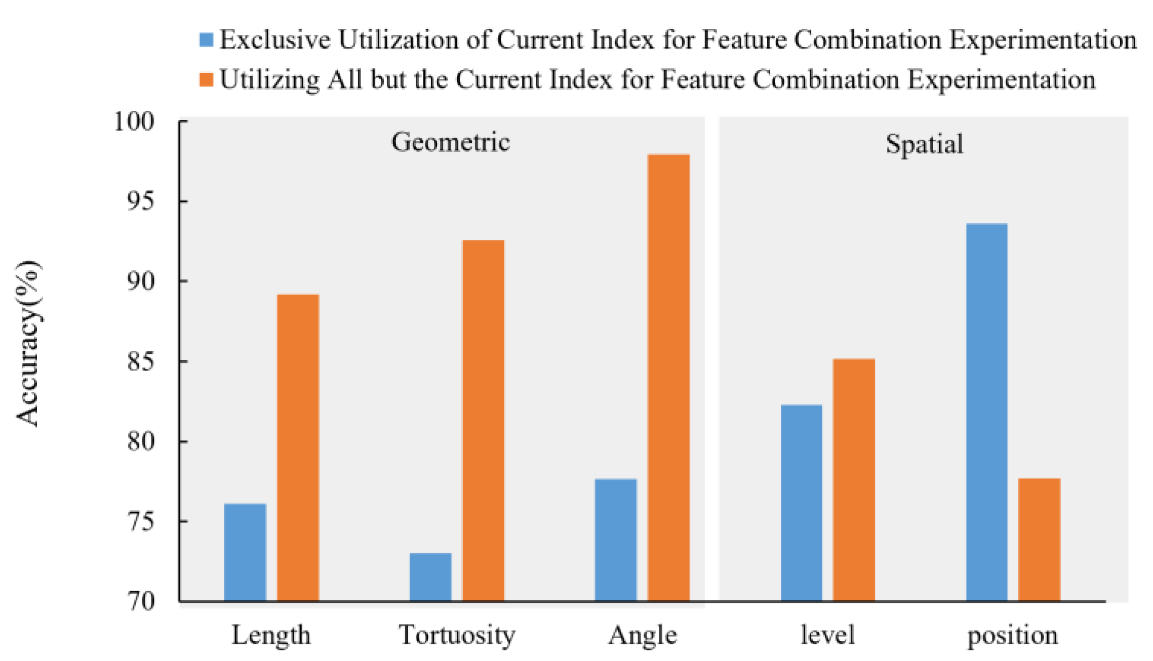
Feature selection plays a crucial role in the success of model training in machine learning tasks. Some features may be highly informative, while others may have less importance. To investigate the impact of feature selection on model classification in the context of river network samples, we conducted parameter sensitivity experiments. Figure 9 shows the accuracy of model training and prediction using only a specific feature or after removing that feature. The features were categorized into geometric features and spatial features. When using only a single geometric feature for classification, the model achieved classification accuracies below 80% on the testing set, indicating that solely relying on geometric features of the river network is insufficient for effective classification. However, when using individual spatial features, the model achieved classification accuracies above 80%. Specifically, when using the hierarchy feature and position feature alone, the model achieved classification accuracies of 82.26% and 93.57%, respectively. In the feature combination experiments, removing a single geometric feature had limited impact on the model’s classification performance, with the accuracy remaining at around 90%. On the other hand, removing a single spatial feature significantly decreased the model’s classification performance. After removing the hierarchy feature and position feature separately, the prediction accuracies were 85.15% and 77.69%, respectively. These results indicate that spatial features of the river network play a crucial role in the classification performance of the graph-convolution-based river network pattern recognition model. There is a certain degree of correlation among the geometric features used, as removing a single geometric feature still maintained decent classification performance. Additionally, it is worth mentioning that existing graph convolution methods often cannot effectively utilize edge attributes in the graph structure and cannot solely use edge attributes as input to the convolutional layer. Therefore, when training the model using the angle feature alone, we assigned the angle between the current node and its parent node (with the angle attribute of the root node set to 0) as the input attribute value for the model.

4. Conclusions and Outlook

Drainage pattern recognition is a challenging task that involves complexity and diversity. In the task of river network pattern recognition, it is necessary to consider various characteristics of the river network, such as semantics, geometry, topology, local features, and global features, in order to classify the river network effectively. To address this challenge, we propose a river network pattern recognition method based on graph convolutional networks, which provides a new approach to tackle this problem. By combining spatial and geometric features of river networks and utilizing graph convolutional models, we are able to extract crucial features from the data and achieve accurate classification of four different river network patterns, including dendritic, trellis, comb-like, and fan-like patterns.
Upon analysis and summarization, the characteristics of our proposed river network pattern recognition method are as follows:
(1)
Introducing graph convolutional networks (GCNs) as a deep learning approach to tackle the pattern recognition problem of drainage networks. This method employs case-based learning, training on manually labeled cases, effectively leveraging expert experience and knowledge. It alleviates the burden of feature engineering to some extent, enhancing the intelligence- and knowledge-based aspects of drainage network pattern recognition. Compared to previous research methods, the GCN-based approach can utilize and learn the spatial and topological features of the river network, automatically extracting and updating node feature representations during the learning process, thereby improving the accuracy of pattern recognition.
(2)
Experimental results demonstrate that spatial features of drainage networks play an equally important role in pattern recognition tasks within GCNs and other deep learning methods. This finding provides valuable insights for future research, suggesting that further utilization of spatial features in river networks can enhance the accuracy and performance of pattern recognition.
(3)
The pattern recognition model based on a GCN exhibits strong learning capabilities. As the quality and quantity of different types of sample data increase, along with improvements in the description of river network features, this method is expected to further enhance recognition performance.
Furthermore, it is important to reiterate that in this study, we believe there are certain primary and recurrent fundamental types of river networks, along with their derived types. Therefore, the sample selection was not solely based on real watersheds but rather aimed to address the issue of uneven quantities and sizes of different types of river networks. This approach was taken to enhance the classification performance of the deep-learning-based model. Furthermore, this methodology provides a new perspective for future research, wherein more precise sample selection and comprehensive data coverage can be employed to further explore and leverage the morphological features of river networks, thereby improving and expanding the deep-learning-based river network pattern recognition methods.
We have reasons to believe that the graph-convolution-based river network pattern recognition framework can be effective in more complex river network pattern recognition tasks when appropriate classification metrics are selected. However, there are still several limitations that need further improvement in future research:
(1)
We structured the river network data based on river reaches as the fundamental units, which yielded promising results. In future studies, it is possible to construct a more geographically meaningful river network data structure by considering entire river entities as the basic units. This can be beneficial for pattern recognition and other related tasks.
(2)
The sample selection process in our research only considered a subset of typical river network types. In the future, it is important to expand the range of river network types studied to encompass a wider variety.
(3)
Understanding the influence of scale effects on the recognition of drainage networks is also an important aspect that can be further explored in future research.
(4)
Composite forms of drainage networks were not included in this study. In the future, these networks can be identified by delineating watershed areas into smaller drainage networks and then performing pattern recognition on them.
Addressing these limitations will contribute to the further development and enhancement of river network pattern recognition methodologies based on graph convolution.

Author Contributions

Conceptualization, Pengcheng Liu; methodology, Pengcheng Liu and Xiaofeng Xu; software, Xiaofeng Xu; validation, Xiaofeng Xu; formal analysis, Mingwu Guo; investigation, Pengcheng Liu and Xiaofeng Xu; data curation, Mingwu Guo; writing–original draft preparation, Xiaofeng Xu; writing–review and editing, Mingwu Guo; visualization: Xiaofeng Xu; supervision, Pengcheng Liu; project administration, Pengcheng Liu; funding acquisition, Pengcheng Liu. All authors have read and agreed to the published version of the manuscript.

Funding

This research was funded by the National Natural Science Fund of China, grant number 42071455.

Data Availability Statement

The data that support the findings of this study are openly available. https://doi.org/10.6084/m9.figshare.14938776.v1 (accessed on 9 July 2021).

Conflicts of Interest

The authors declare no conflict of interest.

References

  1. Tan, X.; Wu, F.; Huang, Q.; Deng, H.Y. A Multi-criteria Decision Model for Identifying Master River and Its Application in River System Construction. Acta Geod. Cartogr. Sin. 2005, 34, 154–160. (In Chinese) [Google Scholar]
  2. Tan, W.; Xing, J.; Yang, S.; Yu, G.; Sun, P.; Jiang, Y. Long Term Aquatic Vegetation Dynamics in Longgan Lake Using Landsat Time Series and Their Responses to Water Level Fluctuation. Water 2020, 12, 2178. [Google Scholar] [CrossRef]
  3. Touya, G. River network selection based on structure and pattern recognition. In Proceedings of the 23rd International Cartographic Conference, Moscow, Russia, 4–10 August 2007. [Google Scholar]
  4. Strahler, A.N. Hypsometric (Area-Altitude) Analysis of Erosional Topography. Geol. Soc. Am. Bull. 1952, 63, 1117–1141. [Google Scholar] [CrossRef]
  5. Shreve, R.L. Statistical law of stream numbers. J. Geol. 1966, 74, 17–37. [Google Scholar] [CrossRef]
  6. Scheidegger, A.E. The algebra of stream-order numbers. U. S. Geol. Surv. Prof. Pap. 1965, 525, 187–189. [Google Scholar]
  7. Woldenberg, M.J. Spatial order in fluvial systems: Horton’s laws derived from mixed hexagonal hierarchies of drainage basin areas. Geol. Soc. Am. Bull. 1969, 80, 97–112. [Google Scholar] [CrossRef]
  8. Jarvis, R.S. Drainage network analysis. Prog. Phys. Geogr. 1977, 1, 271–295. [Google Scholar] [CrossRef]
  9. Smart, J. The analysis of drainage network composition. Earth Surf. Process. 1978, 3, 129–170. [Google Scholar] [CrossRef]
  10. Guo, Q.S. Analyzing the Characters of the Networks of Rivers and Structuralizing the Tree-like Network of Rivers Automatically. Surv. Mapp. Geol. Miner. Resour. 1999, 4, 5–9. (In Chinese) [Google Scholar]
  11. Argialas, D.; Lyon, J.; Mintzer, O. Quantitative description and classification of drainage patterns. Photogramm. Eng. Remote Sens. 1988, 54, 505–509. [Google Scholar]
  12. Ichoku, C.; Chorowicz, J. A numerical approach to the analysis and classification of channel network patterns. Water Resour. Res. 1994, 30, 161–174. [Google Scholar] [CrossRef]
  13. Snelder, T.H.; Biggs, B.J.F.; Woods, R.A. Improved eco-hydrological classification of rivers. River Res. Appl. 2005, 21, 609–628. [Google Scholar] [CrossRef]
  14. Du, Q.Y.; Yang, P.F.; Tan, R.C. Classification of River Networks Structure Based on Spatial Statistical Character. Geomat. Inf. Sci. Wuhan Univ 2006, 31, 419–422. (In Chinese) [Google Scholar]
  15. Zhang, L.; Guilbert, E. Automatic drainage pattern recognition in river networks. Int. J. Geogr. Inf. Sci. 2013, 27, 2319–2342. [Google Scholar] [CrossRef] [Green Version]
  16. Jung, K.; Shin, J.-Y.; Park, D. A new approach for river network classification based on the beta distribution of tributary junction angles. J. Hydrol. 2019, 572, 66–74. [Google Scholar] [CrossRef]
  17. Mejía, A.I.; Niemann, J.D. Identification and characterization of dendritic, parallel, pinnate, rectangular, and trellis networks based on deviations from planform self-similarity. J. Geophys. Res. Earth Surf. 2008, 113, F02015. [Google Scholar] [CrossRef] [Green Version]
  18. Huang, B.; Zhao, B.; Song, Y. Urban land-use mapping using a deep convolutional neural network with high spatial resolution multispectral remote sensing imagery. Remote Sens. Environ. 2018, 214, 73–86. [Google Scholar] [CrossRef]
  19. Feng, Y.; Thiemann, F.; Sester, M. Learning Cartographic Building Generalization with Deep Convolutional Neural Networks. ISPRS Int. J. Geo-Inf. 2019, 8, 258. [Google Scholar] [CrossRef] [Green Version]
  20. Touya, G.; Lokhat, I. Deep Learning for Enrichment of Vector Spatial Databases. ACM Trans. Spat. Algorithms Syst. 2020, 6, 1–21. [Google Scholar] [CrossRef] [Green Version]
  21. Yan, X.; Ai, T.; Yang, M.; Yin, H. A graph convolutional neural network for classification of building patterns using spatial vector data. ISPRS J. Photogramm. Remote Sens. 2019, 150, 259–273. [Google Scholar] [CrossRef]
  22. Donadio, C.; Brescia, M.; Riccardo, A.; Angora, G.; Veneri, M.D.; Riccio, G. A novel approach to the classification of terrestrial drainage networks based on deep learning and preliminary results on solar system bodies. Sci. Rep. 2021, 11, 5875. [Google Scholar] [CrossRef] [PubMed]
  23. Yu, H.; Ai, T.; Yang, M.; Huang, L.; Yuan, J. A recognition method for drainage patterns using a graph convolutional network. Int. J. Appl. Earth Obs. Geoinf. 2022, 107, 102696. [Google Scholar] [CrossRef]
  24. Kondolf, G.M.; Piégay, H. Tools in Fluvial Geomorphology; Wiley Blackwell: Hoboken, NJ, USA, 2016; 560p. [Google Scholar]
  25. Shreve, R.L. Stream lengths and basin areas in topologically random channel networks. J. Geol. 1969, 77, 397–414. [Google Scholar] [CrossRef]
  26. Dacey, M. Summary of magnitude properties of topologically distinct channel networks and network patterns. In Random Processes in Geology; Springer: Berlin/Heidelberg, Germany, 1976; pp. 16–38. [Google Scholar]
  27. Du, Q.Y. The Automatic Establishment of Structured River Network in Cartographic Database. J. Wuhan Tech. Univ. Surv. Mapp. 1988, 13, 70–77. (In Chinese) [Google Scholar]
  28. Wang, Z.; Müller, J.C. Line generalization based on analysis of shape characteristics. Cartogr. Geogr. Inf. Syst. 1998, 25, 3–15. [Google Scholar] [CrossRef]
  29. Strahler, A.N. Quantitative analysis of watershed geomorphology. Eos Trans. Am. Geophys. Union 1957, 38, 913–920. [Google Scholar] [CrossRef] [Green Version]
  30. Kipf, T.N.; Welling, M. Semi-supervised classification with graph convolutional networks. arXiv 2016, arXiv:1609.02907. [Google Scholar]
  31. Lee, J.; Lee, I.; Kang, J. Self-attention graph pooling. arXiv 2019, arXiv:1904.08082. [Google Scholar]
  32. Fey, M. 2021. Available online: https://pytorch-geometric.readthedocs.io/en/latest/ (accessed on 10 February 2021).
  33. Horton, R.E. Erosional development of streams and their drainage basins hydrophysical approach to quantitative morphology. Geol. Soc. Am. Bull. 1945, 56, 275–370. [Google Scholar] [CrossRef] [Green Version]
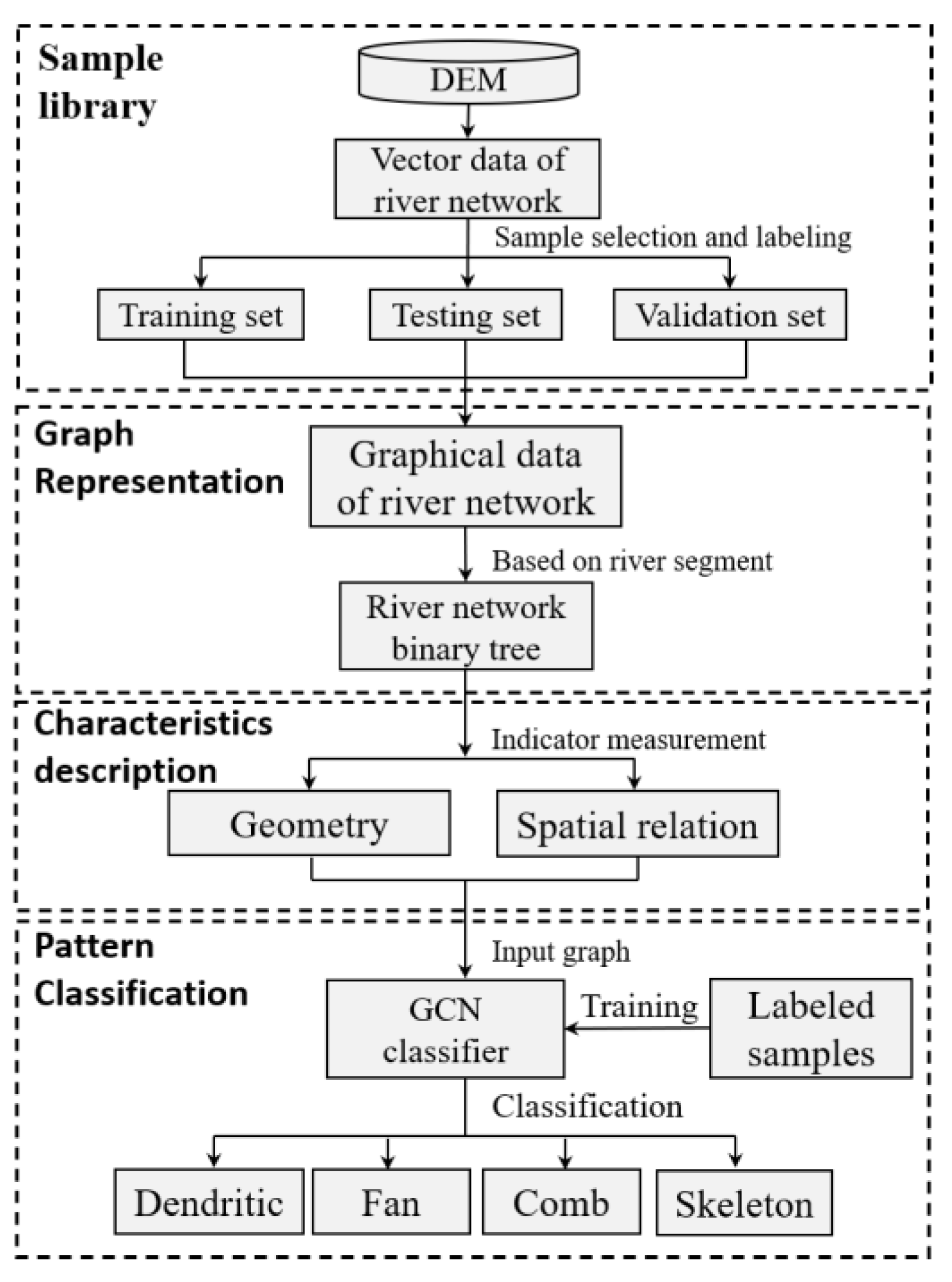
Figure 1. Framework of drainage network pattern recognition.
Ijgi 12 00253 g001
Figure 2. Establishing the binary tree structure of river network: (a) graphic structure of river network; (b) binary tree of the river network. The numbers in the figure represent the visiting order of the river reaches, and furthermore, the right figure is the dual graph of the left figure.
Ijgi 12 00253 g002
Figure 3. The sinuosity of a reach.
Ijgi 12 00253 g003
Figure 4. Calculate the angle between upstream and downstream. AB and BC are simplified representations of the upstream and downstream river segments. BB’ is the extension of AB, and the angle α between BB’ and BC represents the angle between these two river reaches.
Ijgi 12 00253 g004
Figure 5. River network classification model. GC: graph convolution.
Ijgi 12 00253 g005
Figure 6. River network classification model: (a) dendritic network; (b) trellis network; (c) comb-like network; (d) fan-like network.
Ijgi 12 00253 g006
Figure 7. The change in loss value and precision of training set and validation set in the training process.
Ijgi 12 00253 g007
Figure 8. Influence of graph convolution parameters on classification results.
Ijgi 12 00253 g008
Figure 9. Effects of different feature combinations on classification results.
Ijgi 12 00253 g009
Table 1. Characteristic parameters of graph nodes and edges.
Categories of
Indices
CharacteristicsMethod of Calculation or RepresentationNote
Geometric indicesLength l Node properties, the length of river reach
Sinuosity s = d l The degree of bend in the reach
Confluence angleθEdge attribute, angle between reach and upstream reach
Spatial indicesStream orderingNode properties, encoded using Strahler ordering
Left and right position identification x 0 , 1 Node attribute, relative to the left and right position of the downstream stream
Table 2. Confusion matrix.
Predicted ClassTrellisDendriticComb-LikeFan-Like
Actual Class
Trellis88426
Dendritic010000
Comb-like00982
Fan-like10396
Table 3. Pattern recognition results of some samples.
No.ThumbnailLabelPredicted LabelCorrect or WrongPrediction for Different
Types of Probabilities
DendriticTrellisComb-LikeFan-Like
1Ijgi 12 00253 i001DendriticDendriticT0.99680.00320.00000.0000
2Ijgi 12 00253 i002DendriticDendriticT0.99720.00280.00000.0000
3Ijgi 12 00253 i003DendriticDendriticT0.99200.00800.00000.0000
4Ijgi 12 00253 i004DendriticDendriticT0.99370.00630.00000.0000
5Ijgi 12 00253 i005DendriticDendriticT0.99490.00160.00000.0035
6Ijgi 12 00253 i006TrellisTrellisT0.00020.99970.00000.0000
7Ijgi 12 00253 i007TrellisTrellisT0.00150.99690.00000.0016
8Ijgi 12 00253 i008TrellisFan-likeF0.00330.04780.03120.9178
9Ijgi 12 00253 i009TrellisComb-likeF0.00000.00450.99360.0020
10Ijgi 12 00253 i010TrellisDendriticF0.79410.20560.00000.0004
11Ijgi 12 00253 i011Comb-likeComb-likeT0.00000.00001.00000.0000
12Ijgi 12 00253 i012Comb-likeComb-likeT0.00000.00001.00000.0000
13Ijgi 12 00253 i013Comb-likeComb-likeT0.00000.00001.00000.0000
14Ijgi 12 00253 i014Comb-likeFan-likeF0.00130.04780.28170.6693
15Ijgi 12 00253 i015Comb-likeFan-likeF0.00010.01270.00320.9841
16Ijgi 12 00253 i016Fan-likeFan-likeT0.00000.00050.00030.9992
17Ijgi 12 00253 i017Fan-likeFan-likeT0.00000.00000.00001.0000
18Ijgi 12 00253 i018Fan-likeFan-likeT0.00570.10080.00110.8924
19Ijgi 12 00253 i019Fan-likeComb-likeF0.00030.05060.87160.0775
20Ijgi 12 00253 i020Fan-likeTrellisF0.03370.55950.00120.4056
Note: The identifier T or F in the column correct or right indicates whether the prediction result is correct. The probability value corresponding to the predicted result.
Disclaimer/Publisher’s Note: The statements, opinions and data contained in all publications are solely those of the individual author(s) and contributor(s) and not of MDPI and/or the editor(s). MDPI and/or the editor(s) disclaim responsibility for any injury to people or property resulting from any ideas, methods, instructions or products referred to in the content.