Geometric Constraint-Based and Improved YOLOv5 Semantic SLAM for Dynamic Scenes

Abstract

When using deep learning networks for dynamic feature rejection in SLAM systems, problems such as a priori static object motion leading to disturbed build quality and accuracy and slow system runtime are prone to occur. In this paper, based on the ORB-SLAM2 system, we propose a method based on improved YOLOv5 networks combined with geometric constraint methods for SLAM map building in dynamic environments. First, this paper uses ShuffleNetV2 to lighten the YOLOv5 network, which increases the improved network’s operation speed without reducing the accuracy. At the same time, a pyramidal scene parsing network segmentation head is added to the head part of the YOLOv5 network to achieve semantic extraction in the environment, so that the improved YOLOv5 network has both target detection and semantic segmentation functions. In order to eliminate the objects with low dynamic features in the environment, this paper adopts the method of geometric constraints to extract and eliminate the dynamic features of the low dynamic objects. By combining the improved YOLOv5 network with the geometric constraint method, the robustness of the system is improved and the interference of dynamic targets in the construction of the SLAM system map is eliminated. The test results on the TUM dataset show that, when constructing a map in a dynamic environment, compared with the traditional ORB-SLAM2 algorithm, the accuracy of map construction in a dynamic environment is significantly improved. The absolute trajectory error is reduced by 97.7% compared with ORB-SLAM2, and the relative position error is reduced by 59.7% compared with ORB-SLAM2. Compared with DynaSLAM for dynamic scenes of the same type, the accuracy of map construction is slightly improved, but the maximum increase in keyframe processing time is 94.7%.

1. Introduction

With the rapid development of robotics and computer applications, simultaneous localization and mapping (SLAM) technology [1,2] has been widely used in various fields such as agriculture, unmanned vehicles, and aerospace. In indoor mapping, SLAM technology mainly uses a variety of cameras, radar, and other sensors of different models to perceive the surrounding environment. Since there are moving objects in the indoor scene, these moving objects will have a great impact on the result of indoor map construction in SLAM. Therefore, the current research on SLAM technology is mainly to solve the impact of dynamic objects on it. In the research on the SLAM technique of dynamic feature elimination, some excellent algorithms have emerged. With the deepening of research, SLAM technology has also been developed tremendously, and many SLAM map-building techniques such as VSLAM [3], ORB-SLAM [4], ORB-SLAM2 [5], ORB-SLAM3 [6], DynaSLAM [7], DS-SLAM [8], and RGB-D SLAM [9,10,11] have emerged, but currently, the SLAM system for most of them are built with the static environment as the background. This paper uses the ORB-SLAM2 system as the basis for this study.

The relevant sections of this paper are arranged as follows:

(1).

Describing the work and research progress related to dynamic SLAM;

(2).

Presenting the process of light weighting the deep learning network YOLOV5 and the network structure principle of PSPnet in this paper;

(3).

Detailing the rejection of dynamic objects with static priors using geometric constraints in the keyframes processed by the deep learning network;

(4).

Verifying the accuracy of the SLAM algorithm proposed in this paper for constructing maps in dynamic environments;

(5).

Summarizing the results of the SLAM system in this paper for building maps in dynamic environments.

In most cases, SLAM systems build indoor maps and estimate poses against a static environment. However, most of the real environments have dynamic objects in the environment, and these dynamic objects will inevitably affect the accuracy and quality of the map construction when SLAM systems are used for mapping, which will lead to the failure of the map construction and consequently, the subsequent positioning and navigation will be subject to large errors. Therefore, during the study of SLAM mapping systems in dynamic environments [12], researchers have proposed solutions to the problem of interference of dynamic objects with SLAM mapping systems. There are two main approaches for dynamic objects in the environment. (1), using the geometric approach [13] for dynamic feature removal, and (2), using the semantic segmentation approach [14] for dynamic feature removal. Chenyang Zhang et al. [15] proposed a non-semantic a priori dynamic feature proposed method based on particle filtering for dynamic feature removal in the environment. Its main function is to achieve the segmentation of moving objects. Wenxin Wu et al. [16] proposed a new method of geometry for dynamic feature point removal in SLAM system building. First, the dynamic features are detected by the constrained filtering method in the feature detection region, while the detection and removal of dynamic objects are performed by using depth difference and random sampling consistency (RANSAC) [17]. Hongyu Wei et al. [18] addressed the shortcomings of the current dynamic feature removal methods and proposed a combination of the grid-based motion statistics feature point matching method (GMS) [19] combined with the K-means [20] clustering algorithm to remove dynamic regions by distinguishing between dynamic and static regions; while retaining static regions.

When dynamic features are detected and removed using the geometric approach, problems such as high computational effort and inaccurate detection lead to large errors in the removal of dynamic features. With the development of techniques such as deep learning neural networks, many researchers have also applied them to SLAM systems. Zhanyuan Chang et al. [21] used the deep learning network You Only Look Once (YOLOv4-Tiny) [22] for dynamic target detection to improve the stability of the system when building maps in dynamic environments in SLAM systems, and then used the limit geometry and Lucas Kanade optical flow methods (LK optical flow) [23]. Xu, Yan Wang, et al. [24] used a lightweight semantic segmentation network, Fully Convolutional HarDNet (FcHarDNet), to extract semantic information in the problem of dynamic feature detection and removal, and proposed a method of semantic information combined with multi-view geometry for dynamic target rejection. FENG LI et al. [25] addressed the inaccuracy of SLAM systems for map building in large-scale dynamic environments and proposed a method of using multi-view geometry for dynamic target rejection. Shuangquan HAN et al. [26,27] added the semantic segmentation network pyramidal scene parsing network (PSPNet) [28] to ORB-SLAM2 to obtain keyframes with semantic information; and used the semantic information in the detection of dynamic regions and the rejection of dynamic feature points. Li Yan et al. [29] proposed a dynamic SLAM building method using a combination of geometric constraints and semantic information to improve the robustness and efficiency of the SLAM building system, and also proposed a residual model geometric semantic segmentation module to segment dynamic regions.

When the SLAM system is used to build a map in a dynamic environment, the detection and segmentation of dynamic objects using the geometric constraint method can lead to slow operation of the system due to a large amount of computation, and the geometric constraint method cannot recognize the occlusion when it occurs in the environment. Therefore, the geometric constraint approach can lead to large errors in SLAM systems for building maps in dynamic environments. Many researchers use semantic segmentation networks for the detection and extraction of dynamic features in the environment, and the map-building effect of using semantic segmentation networks in the SLAM building system is relatively better than that of using the geometric constraint method. However, the use of semantic segmentation networks in the SLAM system also suffers from incomplete segmentation, large errors in the semantic segmentation of similar objects, and large errors when the a priori static objects undergo motion, the map constructed by the SLAM system will be disturbed by it on the map and other problems.

To address these problems, this paper proposes a SLAM system based on an improved YOLOv5 target detection network combined with geometric constraints for building maps in dynamic environments. In this paper, the head of the pyramidal scene parsing network (PSPNet) semantic segmentation network is added to the YOLOv5 target detection network, so that the improved YOLOv5 network has both target detection and semantic segmentation functions, and the improved network improves the target detection accuracy and semantic segmentation accuracy compared with the traditional YOLOV5 network. The geometric constraint approach is more sensitive to object motion, as the geometric constraint approach does not work well in highly dynamic scenes, but has higher accuracy in detecting and rejecting low dynamic objects. Therefore, this paper combines the improved network with the geometric constraint method. When the SLAM system in this paper builds a map in a dynamic environment, the improved network is first used to detect and semantically segment the dynamic objects, and then the processed keyframes are further used to a priori whether the keyframes are moving or not using the geometric constraint method, and then the keyframes are rejected. Through the analysis of experimental results, the detection accuracy of dynamic features and the quality of building maps in the dynamic environment of the SLAM system are improved after the keyframes are detected and segmented using the algorithm of rejection in this paper.

2. Principle of the Algorithm

2.1. YOLOv5 Network Improvement

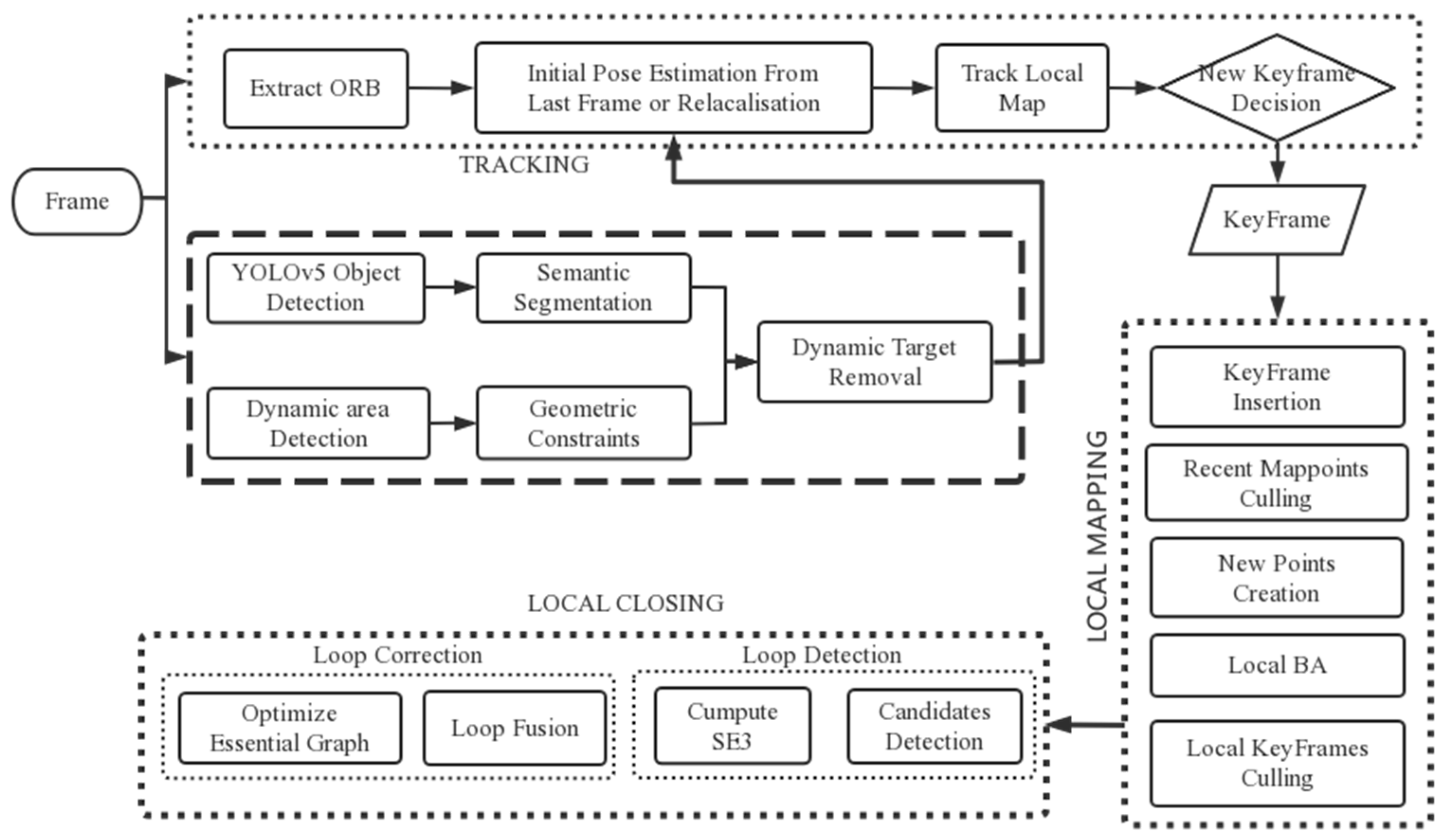
In the SLAM system, the ORB-SLAM2 system has the advantages of simple structure, fast running speed, etc. It is one of the best SLAM systems based on feature point extraction. There are three main threads for map construction using the ORB-SLAM2 system. Based on this, this paper adds a dynamic feature detection thread using the improved YOLOv5 network for map construction. To take advantage of ORB-SLAM2, the algorithm in this paper is improved based on the ORB-SLAM2 algorithm, as shown in the flow chart of this paper in Figure 1.

The algorithm flow of the improved algorithm in this paper is shown in Figure 1. Firstly, when the image collected by the sensor is introduced into the system, ORB feature point matching and dynamic feature point detection are carried out simultaneously. In the process of dynamic feature point detection, the improved YOLOv5 network in this paper is first used for rapid target detection, and objects with dynamic priors are eliminated. For dynamic objects with surprising priors, geometric constraints are used to eliminate their dynamic features. Then, the dynamic feature point detection thread passes the processed image to the tracing thread for initialization and map construction. The mapping process is as follows: firstly, the tracking thread and the thread added in this paper will cull and initialize dynamic feature points of the image, and then select keyframes. The selected keyframes are inserted into the local mapping thread to construct the map, and then the loop closing thread to optimize the global map.

In this paper, three SLAM algorithms are used for experimental testing, and the advantages and disadvantages of each of them are as follows:

The ORB-SLAM2 algorithm is one of the most classic feature point methods in the SLAM algorithm, the ORB-SLAM2 algorithm has good portability and is very suitable for porting to practical projects. The ORB-SLAM2 algorithm uses G2O as an optimization tool at the back end to reduce the feature point location error and the estimation error of its pose, and uses DBOW to reduce the feature, finding that ORB-SLAM2 also has a repositioning function, which can quickly reposition itself when the data stream is interrupted. It has good system tracking and robustness. However, the ORB-SLAM2 algorithm will fail to initialize if the sensor moves too fast to extract features easily during initialization. Additionally, it is easy to lose frames when the rotation or corner is large, sensitive to noise, and also prone to drift and poor accuracy for pure visual SLAM.

DynaSLAM is proposed by Bescos et al. [7]. based on the improvement of ORB-SLAM2, which is mainly used for SLAM systems to build maps in dynamic environments, and it mainly adds dynamic detection and background repair based on ORB-SLAM2. For dynamic detection, the Mask-RCNN deep learning network and geometric methods are used to detect moving and possibly moving objects, respectively. For camera pose estimation, DynaSLAM only uses ORB feature points in static regions and non-dynamic object mask edges, and mainly uses historical observation data for static background restoration. However, DynaSLAM is computationally overloaded in the environment for map building leading to a long running time and long processing time for a single frame, while the method chooses to remove all potentially possible moving objects, which can affect the camera pose estimation.

The SLAM algorithm proposed in this paper is based on ORB-SLAM2 for map construction in dynamic environments, and first uses the lightweight network YOLOv5 for target detection and the semantic segmentation of dynamic objects in the environment to ensure detection accuracy without slowing down the system operation, and uses geometric methods for the detection of low dynamic objects and potential objects. Compared with the ORB-SLAM2 algorithm, the SLAM algorithm proposed in this paper is less prone to frame loss when the camera rotation angle is too large when building maps in dynamic environments. Compared with DynaSLAM, the SLAM algorithm proposed in this paper has the advantages of fast running speed and short processing time for a single frame.

2.2. YOLOv5 Lightweight Network

When constructing the map in the SLAM system, the deep learning network is first used for target detection and the semantic segmentation of the image, because of the high complexity of the deep learning network structure. Image processing will increase the processing time of each frame, and the SLAM system also needs to detect each dynamic feature point when removing dynamic feature points. Therefore, when a deep learning network is added to the SLAM system to build the map in a dynamic environment, the processing time of each frame image will increase. Due to the increase in processing time, it is easy to lose frames, which leads to errors in drawing accuracy, incomplete drawing, and other problems. To improve the image processing speed of the deep learning network YOLOv5 [30], we made improvements based on the YOLOv5 network [31] and carried out lightweight network improvements to improve the running speed and network size of the network. Thus, the accuracy and speed of drawing construction of the SLAM system are improved, and the stability of drawing construction of the SLAM system in a dynamic environment is improved. The structure principle of the improved YOLOv5 network is shown in Figure 2.

The full names of each module are as follows:

(1).

CBR: Conv and BN and ReLU;

(2).

CBL: Conv and BN and Leaky ReLU;

(3).

CBS: Conv and BN and SiLU;

(4).

BN: BatchNorm2d;

(5).

UP: Upsampling;

(6).

DWB: Double Weights and Biases;

(7).

SFP: Spatial Feature Enhancement Block.

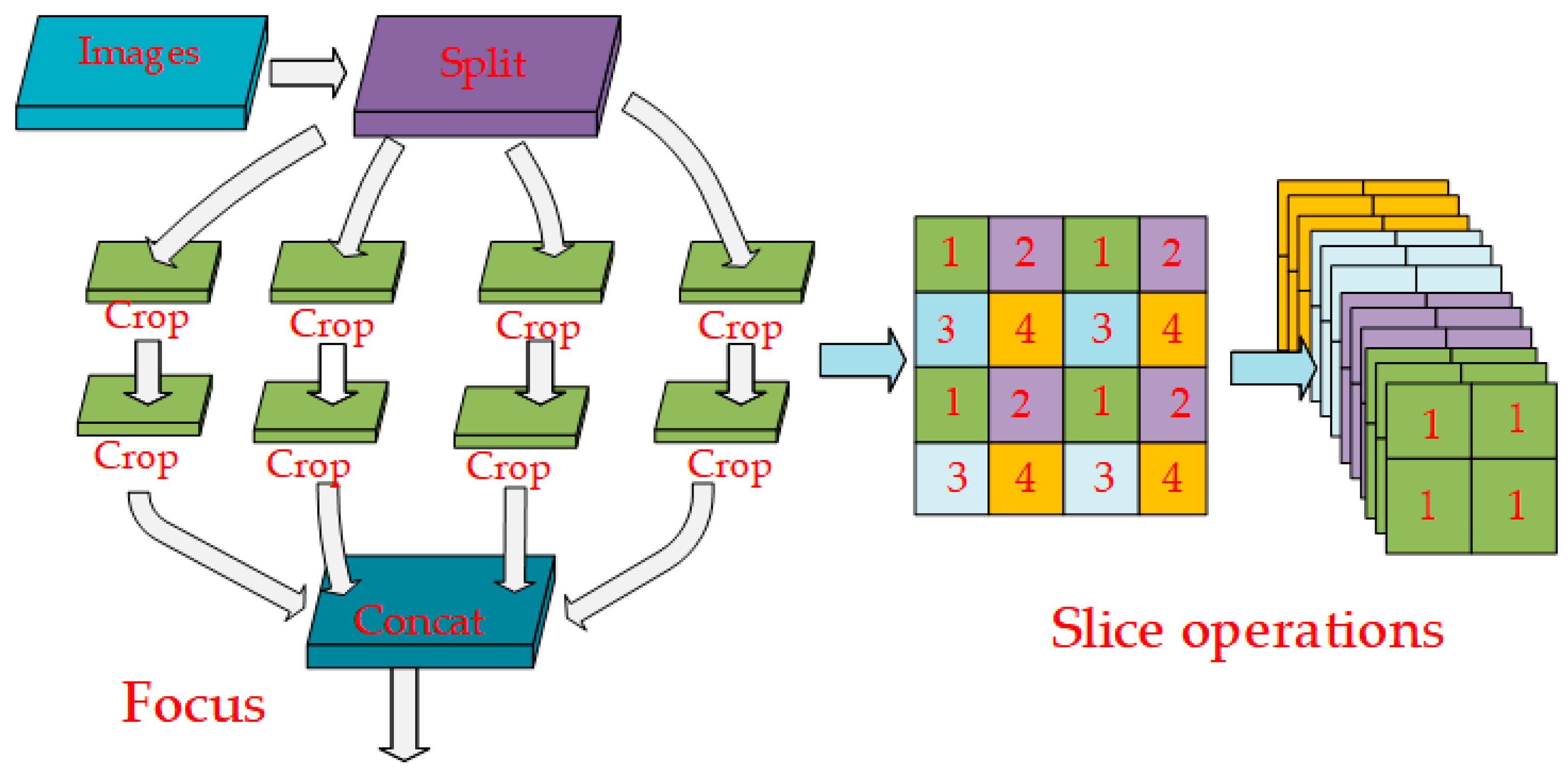
In the base version of YOLOv5, the focus layer consists of four slice operations in the superstructure of feature extraction. To improve the running speed of the YOLOv5 network, this paper uses convolution instead of focus to obtain better performance without some limitations and side effects. Therefore, the focus layer is directly removed in the improved YOLOv5 network. Intuitively speaking, this is to slice the image operation. The improvement principle is shown in Figure 3 below.

ShuffleNet [32,33] is selected in this paper to improve the backbone of YOLOv5. Here are four guidelines for lightweight design:

(1).

The same channel size can minimize memory access;

(2).

Excessive use of group convolution will increase MAC;

(3).

Network fragmentation (especially multiplexing) will reduce the degree of parallelism.

(4).

Element-level operations (such as shortcut and add) cannot be ignored.

Because the C3 layer uses multiplex separation and convolution, the C3 layer and C3 layer with a high number of channels are frequently used, occupying more cache space and reducing the running speed. Therefore, the improved YOLOv5 in this paper avoids multiple uses of C3 layer and C3 layer of high channels in the network.

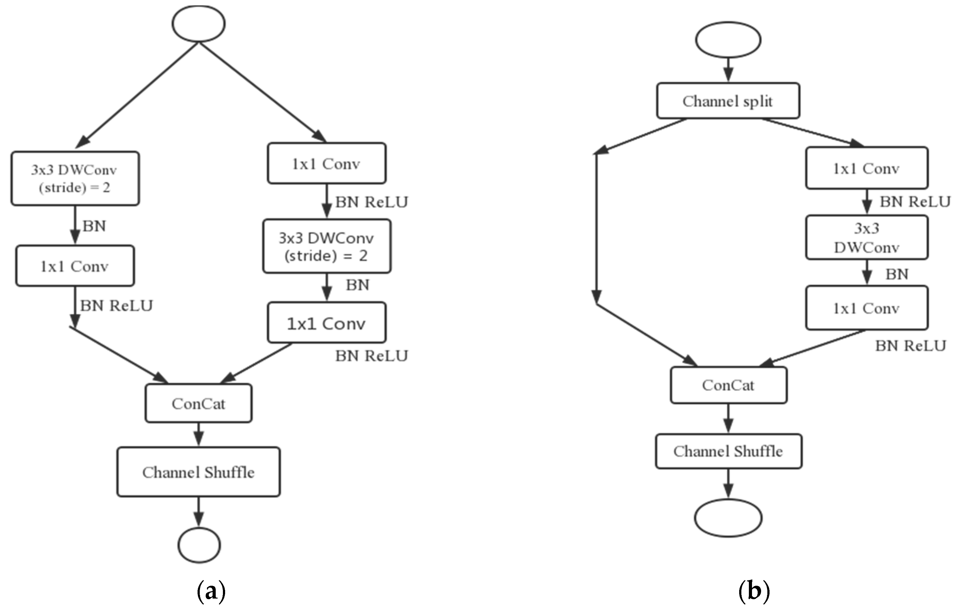
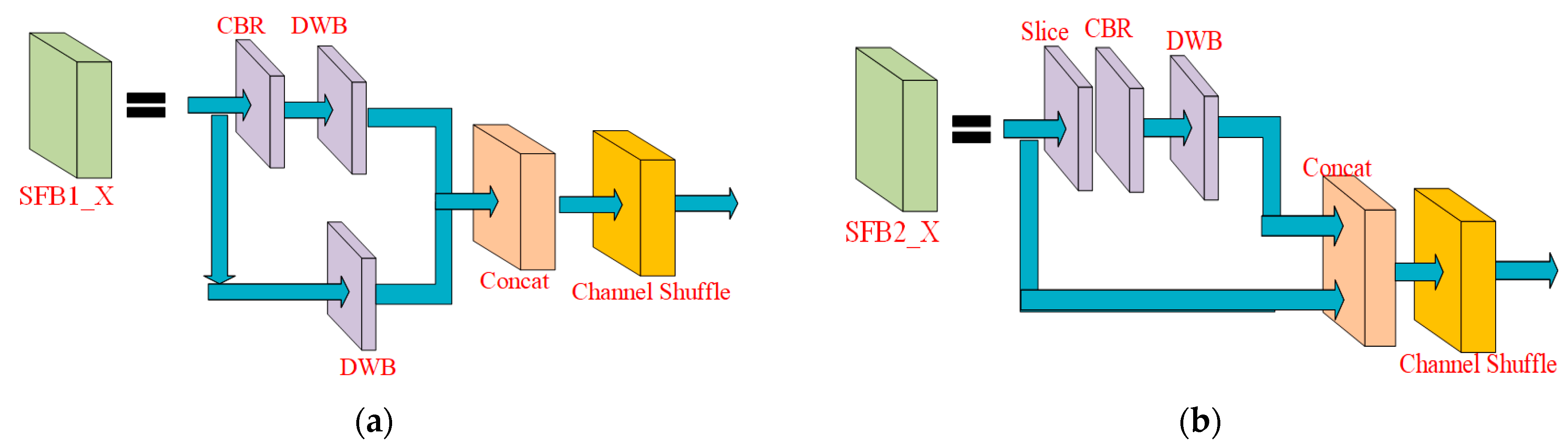
Subfigures (a) and (b) in Figure 4 are the ShuffleNetV2 [34] layer structure and the main structure in the improved YOLOv5 network, corresponding to SFB1_X and SFB2_X, respectively, in Figure 5.

For the focus layer, a feature map with four times the number of channels is generated every four adjacent pixels in a square, which is similar to downsampling operations four times on the upper layer, and then the results are concatenated together. The most important function is to not reduce the feature extraction ability of the model. The model was reduced and accelerated. The improved YOLOv5 in this paper also removes 1024 conv and 5 × 5 pooling of ShuffleNetv2 backbone.

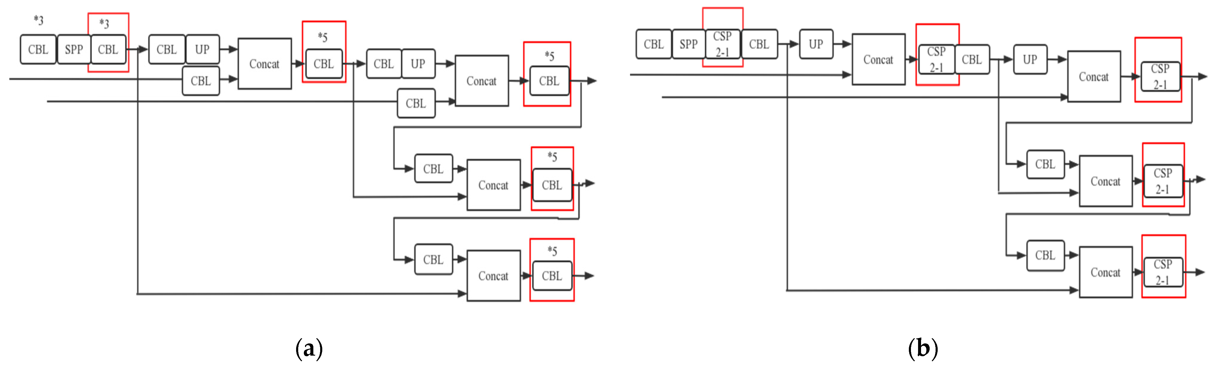
In the head part of YOLOv5, this paper also makes corresponding improvements. PSPNet segmentation header is added in the head part of YOLOv5, realizing that the improved network has both target detection and semantic segmentation functions. In the neck layer of YOLOv4 [29], the structures required by its operations need to be combined with the convolutional network to complete. However, the neck layer of YOLOv5 adopts the CSP2_X structure designed by CSPnet, which makes the YOLOv5 network stronger in terms of feature fusion. Its principle is shown in Figure 6b:

The red boxes in Figure 6a,b indicate the differences between the YOLOv4 network and the YOLOv5 network. The functions of each module in Figure 6 are as follows:

CBL module: convolution and feature extraction of images;

Spatial Pyramid Pooling (SPP) module: avoiding frame loss during image clipping and scaling;

CSP2-1 module: avoiding gradient disappearance;

UP module: integration of images so that the input images are the same size;

Concat module: fusing image features to highlight the detected features.

To improve the accuracy of the results and avoid convergence failures such as $IOU$ and $GIOU$ during network training, the $CIOU$ of the YOLOv5 network can calculate the distance between the target and the anchor frame, as well as the coverage and penalty classes. The formula for $CIOU$ is as follows.

$$CIOU=IOU-\frac{{\rho }^2(b,b^{gt})}{c^2}-\alpha \nu$$

(1)

where ${\rho }^2(b,b^{gt})$ represents the Euclidean lengths of the prediction frame and the true frame form centers, respectively, $c$ is the diagonal length of the range of the prediction frame and the true frame together, $\alpha$ and $\nu$ are given by the following equations.

$$\alpha =\frac{\nu }{1-IOU+\nu }$$

(2)

$$\nu =\frac{4}{{\pi }^2}{(\arctan \frac{{\omega }^{gt}}{h^{gt}}-\arctan \frac{\omega }{h})}^2$$

(3)

Then the corresponding $LOSS$ is:

$$LOS{S}_{CIOU}=1-IOU+\frac{{\rho }^2(b,b^{gt})}{c^2}+\alpha \nu$$

(4)

During the post-processing of the target detection, the YOLOv5 network uses a Gaussian-weighted non-maximum suppression method (NMS) to filter multiple targets. In the initial NMS, the window with a score above the threshold is set to 0. As shown in Equation (5).

$$S_i=\{\begin{array}{l}{s}_i,IoU(M,b_i)<N_t\\ 0,IoU(M,b_i)\ge N_t\end{array}$$

(5)

In the improved Gaussian-weighted NMS, the anchor boxes with the highest score scores in (5) need to be further processed. The algorithm in this paper sorts the different anchor frames according to their confidence scores instead of deleting them directly, thus allowing the better selection of anchor frames and largely avoiding missing and wrong selections.

2.3. Semantic Segmentation by Fusing PSPNet

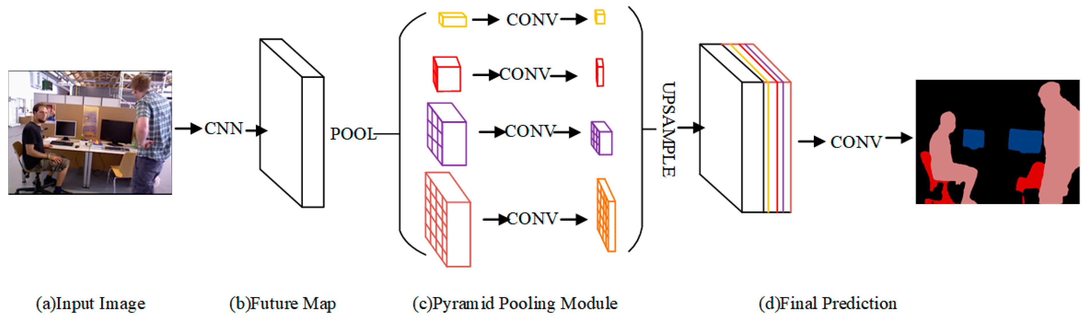
Since the traditional YOLOv5 network can only perform target detection without any semantic information and cannot perform semantic segmentation, this paper adds a PSPNet segmentation layer to the YOLOv5 network to achieve more accurate segmentation at the pixel level. Figure 7 shows the PSPNet network structure.

CNN is a pre-trained model (ResNet101) and a null convolution strategy, which is used to implement the extraction of the feature map, the extracted feature map is 1/8 of the size of the input, the feature map is passed through the Pyramid Pooling module to obtain the fused feature with overall information, which is upsampled with the feature map and is concatenated with the feature map before pooling, and finally, the final output is obtained by a convolution layer. The module fuses four different pyramid scale features: the first row in yellow is the coarsest feature global pooling to generate a single bin output, and the next three rows are the pooled features of different scales. To ensure the weight of the global features, if the pyramid has a total of N levels, a 1 × 1 convolution is used after each level to reduce the four-level channel to the original 1/N. The size before unspooling is then obtained by bilinear interpolation and finally concatenated together. The size of the pooling kernel for the pyramid levels is settable, which is related to the input sent to the pyramid. The kernel sizes are 1 × 1, 2 × 2, 3 × 3, and 6 × 6 for the four ranks used in the paper.

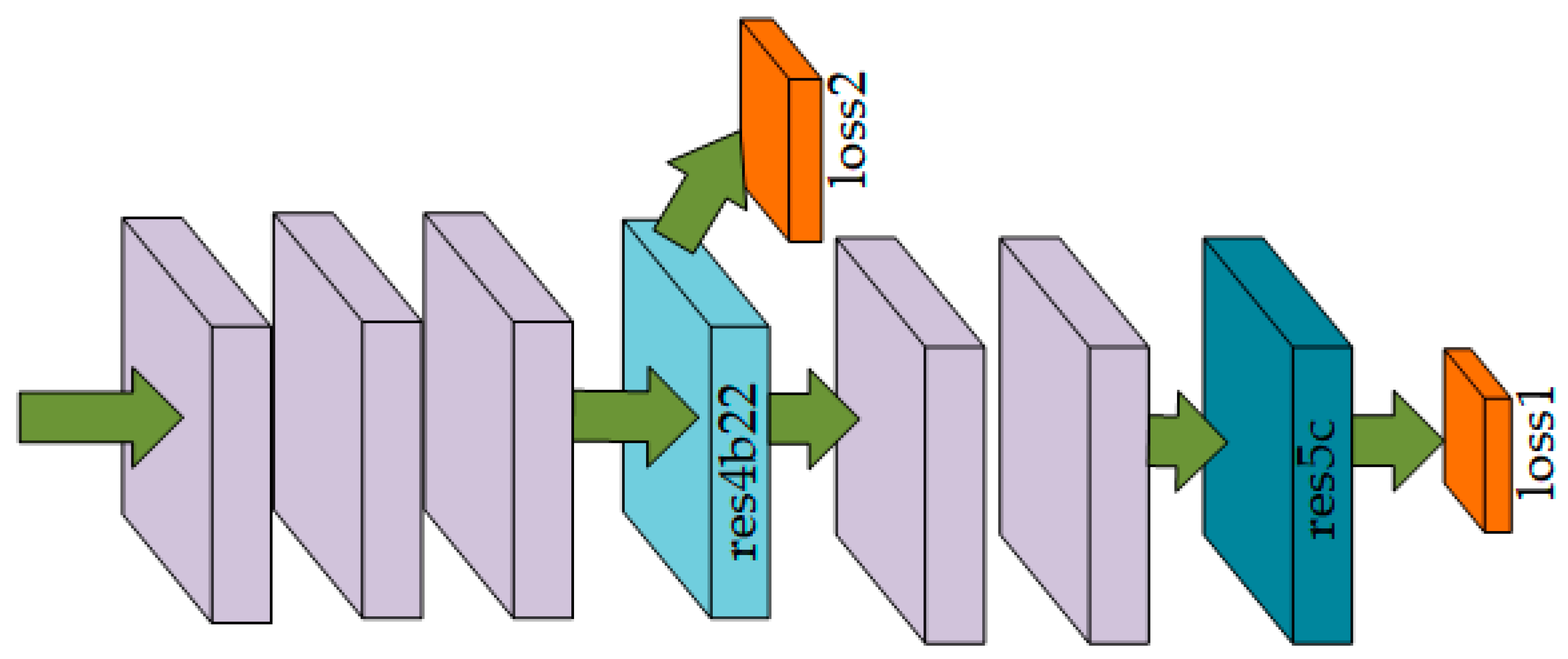
In this paper, some improvements are made on top of the original residual network, where we propose to generate the initial results through an additional loss function and then learn the residuals through the final loss function. Therefore, the optimization problem of the deep network can be decomposed into two, and the solution to a single problem will be simpler. The improved results of the backbone residual network are shown in Figure 8.

In the figure above, an example of our ResNet101 model after adding the auxiliary loss function is given. In addition to training the main branch of the final classifier using softmax loss, another classifier is applied after the fourth stage (the res4b22 residual block). Error backpropagation blocks the auxiliary loss function from passing to the shallower network layers, and we let both loss functions pass through all network layers before it. The auxiliary loss function helps to optimize the learning process, while the main branch loss function takes the greatest responsibility. Finally, we also add weights to balance the auxiliary loss function. That is, the two losses are propagated together, using different weights, to jointly optimize the parameters, which facilitates fast convergence.

The training results of the network in this paper are shown in Figure 9:

3. Principle of Dynamic Feature Removal Method

The geometric constraint approach can achieve good results in low dynamic environments when dynamic feature points are removed. However, when the object motion is relatively fast, the geometric constraint approach is prone to errors. In most dynamic environments, the interference of dynamic features to the SLAM system can be effectively solved by using the deep learning approach, but the system retains a large number of dynamic points when the a priori stationary objects move. Therefore, this paper uses a combination of geometric constraints and deep learning to reject dynamic feature points and improve the accuracy and robustness of the system.

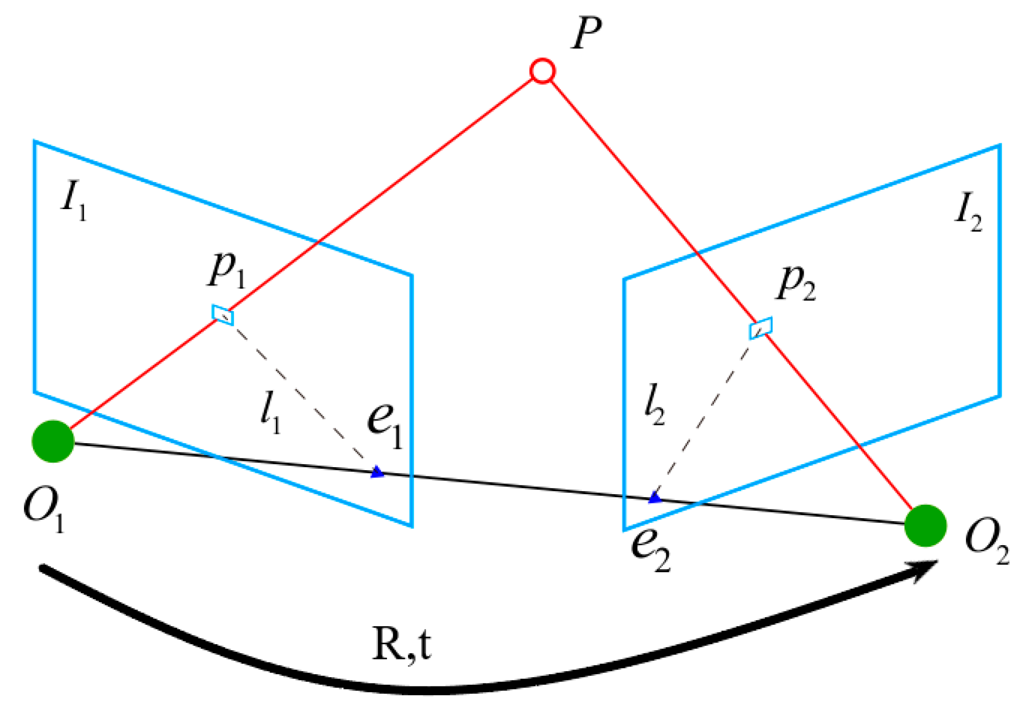
According to Figure 10 [35], let $P$ be a point in space, $p_1$ the projection point of space point p on the first image frame, and $p_2$ the projection point of space point p on the second image frame, point $e_1$ and point $e_2$ are poles, and the line between projection point $p_1$ and pole $e_1$ becomes a polar line $l_1$, and the line between projection point $p_2$ and pole $e_2$ becomes a polar line $l_2$. The motion from the first frame to the second frame is the rotation matrix $R$ and the translation vector $t$, and the two camera centers are $O_1$ and $O_2$, respectively. Now, consider that there is a feature point $p_1$ in the first frame image, which corresponds to the feature point $p_2$ in the second image. According to the camera motion, we can obtain the feature points $p_1$, $p_2$ by feature matching, which means they are the projections of points at the same position in space on two imaging planes.

The spatial position of the point $P$ under the coordinate system of the first image is noted as $(x,y,z)$, and according to the pinhole camera model, its pixel coordinates $p_1$, $p_2$ on the two images are

$$s_1{p}_1=KP$$

(6)

$$s_2{p}_2=K(RP+t)$$

(7)

where $K$ is the camera internal reference matrix, $R,t$ is the motion between two camera coordinate systems, which represents the conversion of coordinates under coordinate system 1 to coordinate system 2, and they are the quantities to be found. $p_1,p_2$ is the pixel point flush coordinates, which are obtained by feature extraction and matching.

Let $x_1,x_2$ be the coordinate on the normalized plane corresponding to the pixel $p_1,p_2$:

$$x_1=K^{-1}{p}_1$$

(8)

$$x_2=K^{-1}{p}_2$$

(9)

Substituting Equation (9) into Equation (8), we obtain

$$x_2=R{x}_1+t$$

(10)

The simultaneous left multiplication of both sides by $t^{\wedge }$ is equivalent to the simultaneous outer product of both sides with $t$.

$$t^{\wedge }{x}_2=t^{\wedge }R{x}_1$$

(11)

Both sides simultaneously left multiply $x_2^T$:

$$x_2^T{t}^{\wedge }{x}_2=x_2^T{t}^{\wedge }R{x}_1$$

(12)

Looking at the left side of Equation (12), the $t^{\wedge }{x}_2$-vector is perpendicular to both vector $t$ and vector $x_2$. When the vector is made an inner product with the vector, the result is 0. When making the inner product with vector $x_2$, the result is 0. Therefore, Equation (12) can be written as

$$x_2^T{t}^{\wedge }R{x}_1=0$$

(13)

Substituting into $p_1,p_2$, we have

$$p_2^T{K}^{-T}{t}^{\wedge }R{K}^{-1}{p}_1=0$$

(14)

The middle part of the mathematical expression for the pair–pole constraint is written as two matrices, which can further simplify the pair–pole constraint:

$$\{\begin{array}{l}E=t^{\wedge }R\\ F=K^{-T}E{K}^{-1}\\ x_2^{T}E{x}_1=p_2^{T}F{p}_1=0\end{array}$$

(15)

In Equation (15), $F$ denotes the basis matrix for the transformation of coordinate $O_1$ to coordinate $O_2$ and $E$ is the essence matrix. Therefore, the rotation matrix $R$ and the translation vector $t$ between the two coordinate systems can be calculated according to Equation (13).

In the rejection of dynamic feature points, the distance between the pixel coordinates $p_2$ and the polar line $l_2$ is calculated. If the calculated distance is greater than the set threshold $\mu$, then it is considered as a dynamic feature point for rejection.

$$l_2=\left(\begin{array}{c}a\\ b\\ c\end{array}\right)=F{p}_1$$

(16)

Equation (16), $a,b,c$ represents the coordinate vector of the polar line $l_2$, and then calculate the distance between the pixel coordinate point $p_2$ and the polar line $l_2$, denoted by $d$.

$$d=\frac{\left|p_2^T{l}_2\right|}{\sqrt{a^2+b^2}}$$

(17)

When the result $d>\mu$ is calculated, it means that the pixel coordinate point $p_2$ is not on the polar line $l_2$, it is a dynamic feature point and needs to be eliminated.

In the SLAM system, there are three commonly used feature extraction methods, namely SIFT, SURF, and ORB. Scale-invariant feature transform (SIFT) is a method used to detect and describe local features in an image. The key points found by SIFT are points that are very prominent and will not be changed by factors such as illumination, affine transformation, and noise, for example, corner points, edge points, bright points in dark areas, and dark points in bright areas, so its application scenarios are limited. The shortcoming of SIFT is that its real-time performance is not high, and its feature point extraction ability is weak for targets with smooth edges. Speeded-Up Robust Features (SURF) was developed to a large extent to improve the SIFT algorithm and improve the execution efficiency of the algorithm. SURF uses the determinant values of the Hessian matrix for feature point detection and an integral graph to improve the operation speed. SURF relies too much on the gradient direction of pixels in local areas, resulting in an increase in the number of mismatches. Meanwhile, the pyramid layers are not tightly obtained, resulting in scale errors. ORB (Oriented FAST and BRIEF) is a feature detection algorithm proposed on the basis of the famous FAST feature detection and BRIEF feature descriptor. Its running time is much better than SIFT and SURF, and it can be applied to real-time feature detection. The feature detection of ORB is invariant to scale and rotation, as well as to noise and perspective transformation. Good performance means that ORB can be used in a wide range of application scenarios for feature description. In this paper, the improved YOLOv5 network combined with geometric constraints is used to eliminate dynamic features in the environment. Experimental verification shows that the proposed algorithm has obvious advantages in eliminating dynamic features in the environment compared with SLAM algorithms of the same type. 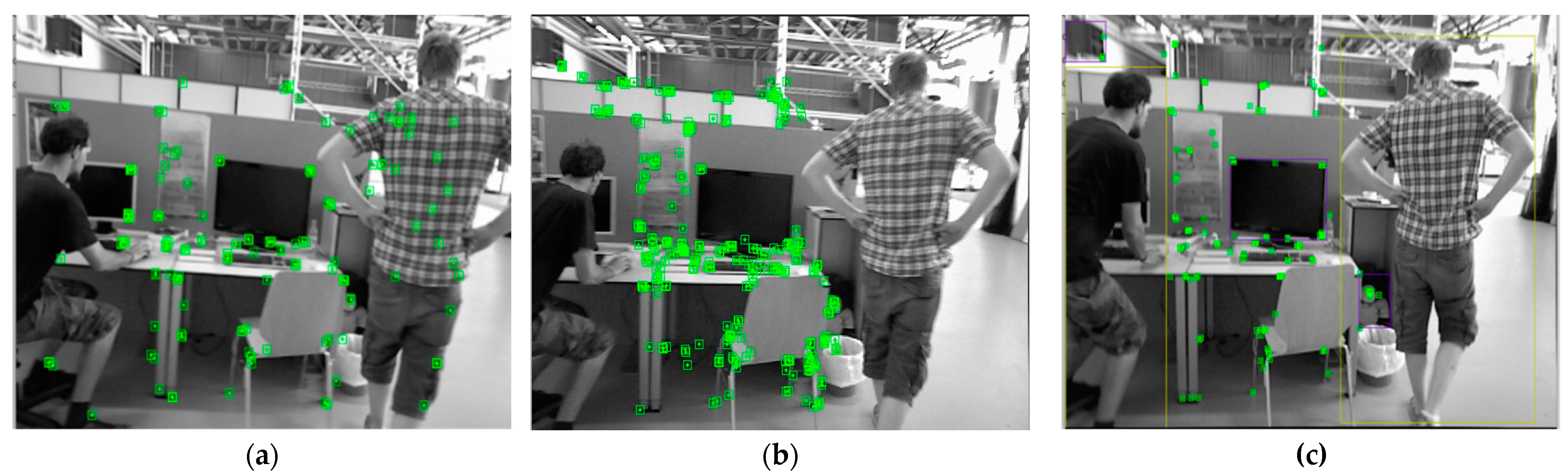The dynamic feature point elimination results of the algorithm in this paper are shown in Figure 11c, and the dynamic feature elimination results of the ORB-SLAM2 algorithm and the DynaSLAM algorithm are shown in Figure 11a,b, respectively.

The results of running the algorithm in this paper with ORB-SLAM2 and DynaSLAM are shown in Figure 11 below.

It is obvious from Figure 11a that ORB-SLAM2 cannot eliminate dynamic feature points in a dynamic environment, and ORB-SLAM2 is only suitable for building maps in a static environment when building maps. Figure 11b shows the feature point rejection results of DynaSLAM in the dynamic environment, which has a great advantage over the feature point rejection results of ORB-SLAM2, and the feature points on people with dynamic features can be well rejected. Figure 11c shows the result of the OurSLAM algorithm in dynamic feature point rejection. Compared with DynaSLAM, OurSLAM has fewer feature points when the algorithm is running, so the algorithm runs faster and the accuracy of the algorithm can be guaranteed at the same time.

4. Algorithm Accuracy Verification

The data used in this paper are from the publicly available TUM dataset. In this paper, five datasets, namely fr3_w_xyz, fr3_w_halfsphere, fr3_w_static, fr3_w_rpy, and fr3_s_static, are used to test the accuracy of this algorithm in a dynamic environment. In this paper, the five datasets are used to test the accuracy of ORB-SLAM2, DynaSLAM, and three SLAM algorithms of OurSLAM improved in this paper. At the same time, absolute trajectory error (ATE) and relative pose error (RPE) are used to evaluate the algorithm accuracy of OurSLAM. To verify the running time of this algorithm per frame, the image processing time per frame of OurSLAM was evaluated through comparative analysis with DynaSLAM run time to verify the running speed of this algorithm.

When evaluating the accuracy of the algorithm, the direct method is generally adopted to evaluate the superiority of the algorithm by comparing the effect of the constructed map. However, for DynaSLAM and OurSLAM algorithms of the same type, the direct approach is far too inaccurate to be able to tell the difference between map construction with the naked eye. Therefore, in this paper, root means square errors (RMSE) of the three algorithms of ORB-SLAM2, DynaSLAM, and OurSLAM are calculated to represent the accuracy of map construction. The formula is as follows:

$$RMSE(E_{1:n},△)={[\frac{1}{m}{\displaystyle \sum _{i=1}^m{\Vert trans(E_i)\Vert }^2}]}^{1/2}$$

(18)

where $trans(E_i)$ denotes the error at $i$ time, $E_{1:n}$ denotes the camera pose from 1 to n, and Δ denotes the fixed time interval, $m$ denotes the numbers of samples. The amount of improvement relative to the ORB-SLAM2 algorithm in this paper is denoted by improvements.

$$improvement=\frac{\mu -r}{\mu }\times 100\%$$

(19)

where $\mu$ denotes $RMSE$ or $SD$ for ORB-SLAM2; $r$ denotes $RMSE$ or $SD$ for OurSLAM.

$RMSE$ and $SD$ of five datasets on three algorithms of ORB-SLAM2, DynaSLAM, and OurSLAM can be obtained through the calculation results of Equations (18) and (19). Since system robustness is very sensitive to outliers in data, $RMSE$ is used in this paper to evaluate system robustness. When evaluating the dispersion of trajectory, this paper uses $SD$ for evaluation, so that the stability of the system can be more clearly judged. The results are shown in

Table 1. Absolute trajectory error comparison results (ATE).

Datasets	ORB-SLAM2		OurSLAM		Improvement/%
	RMSE	SD	RMSE	SD	RMSE	SD
fr3_w_xyz	0.6395	0.3162	0.0139	0.0071	97.8	97.8
fr3_w_halfsphere	0.6685	0.3385	0.0158	0.0153	94.6	95.5
fr3_w_static	0.4165	0.1742	0.0171	0.0043	94.8	97.5
fr3_w_rpy	0.7968	0.4520	0.4439	0.2350	44.3	48.0
fr3_s_static	0.0087	0.0043	0.0066	0.0033	24.1	23.3

and

Table 2. Comparison results of relative positional error (RPE).

Datasets	ORB-SLAM2		OurSLAM		Improvement/%
	RMSE	SD	RMSE	SD	RMSE	SD
fr3_w_xyz	0.0489	0.5243	0.0198	0.0095	59.5	98.2
fr3_w_halfsphere	0.0536	0.5894	0.0162	0.0238	69.8	96.0
fr3_w_static	0.0498	0.4316	0.0186	0.0061	62.7	98.6
fr3_w_rpy	0.0431	0.0281	0.0159	0.0057	63.1	79.7
fr3_s_static	0.0095	0.0041	0.0063	0.0035	33.7	14.6

.

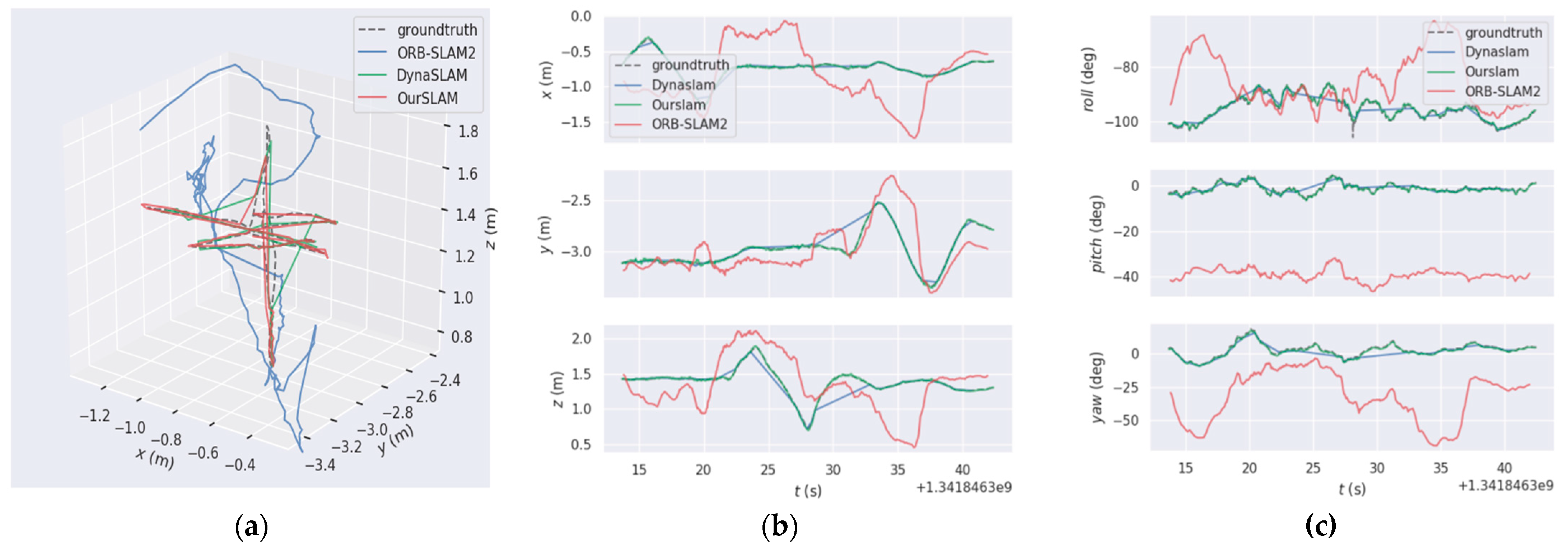
As in Figure 12, in the trajectory map, this paper uses the solid line to represent the real trajectory of the camera motion and the dashed line to represent the predicted trajectory, respectively. From Figure 12a, it can be seen that the ORB-SLAM2 algorithm has almost no trajectory fitting in a dynamic environment. The difference between OurSLAM and DynaSLAM in the trajectory fitting effect is not much, but it can be seen that there is obvious mismatching in the corner direction of the DynaSLAM in X, Y, and Z axis direction, as in Figure 12c in yaw, pitch, and roll. there are still mismatches in yaw, pitch, and roll. Compared with OurSLAM, the predicted trajectory is almost the same as the real trajectory, and the fitting effect is very good, which meets the trajectory accuracy requirement of the dynamic SLAM construction well.

From Figure 12b, we can see that ORB-SLAM2 has almost no overlap with the real trajectory when translating on the three axes, indicating that its trajectory matches the real trajectory with a large error and almost no accuracy. The coincidence of DynaSLAM with the actual trajectory is greatly improved compared with ORB-SLAM2, but a large error occurs when the camera turns too much. The trajectory of OurSLAM translates on the three axes with better coincidence with the real trajectory, and the error is relatively small compared with DynaSLAM. As in Figure 12c, the error is also relatively small when rotating.

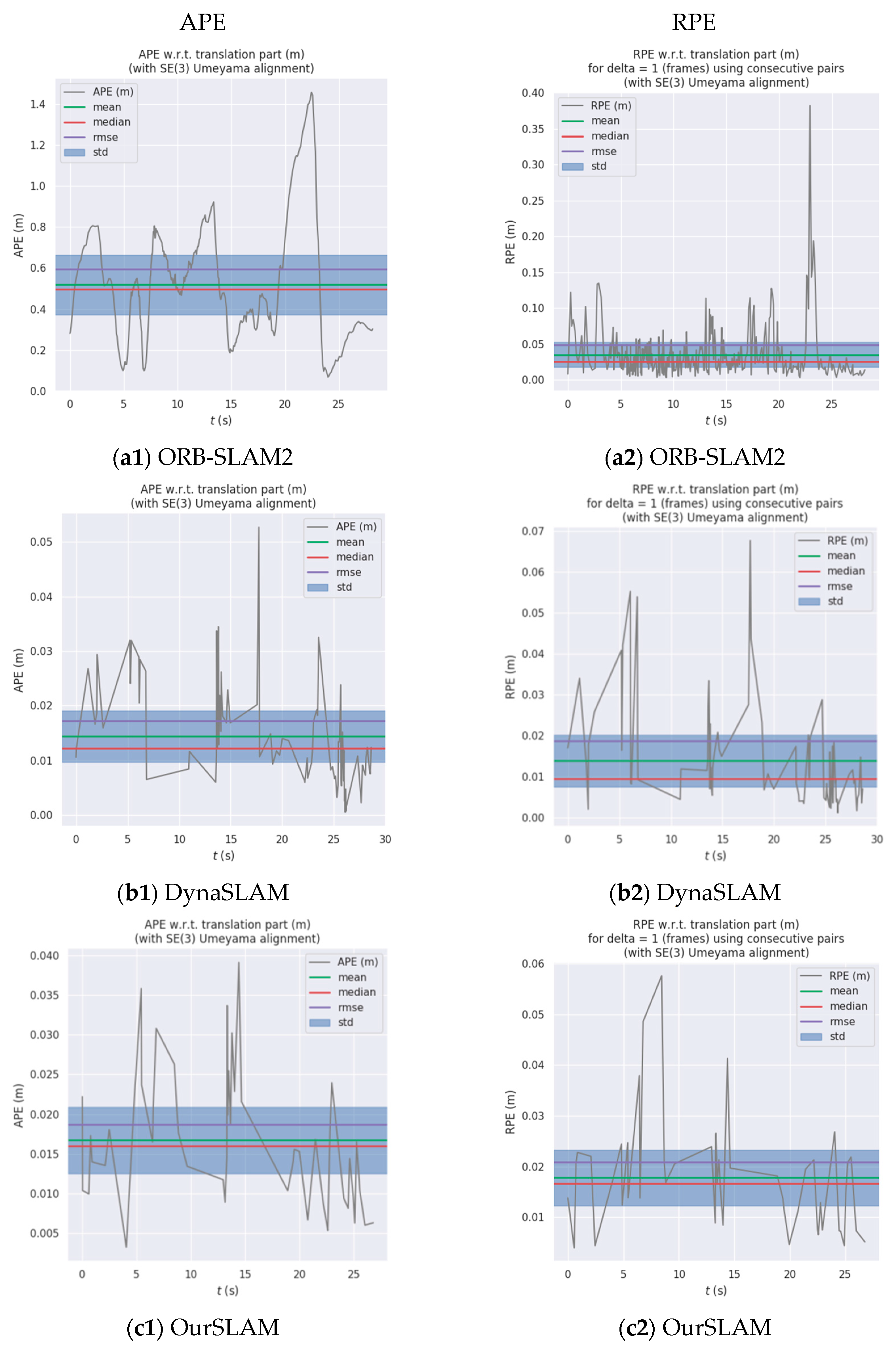
Figure 13 shows the APE and RPE results of ORB-SLAM2, DynaSLAM, and OurSLAM algorithms running on fr3_Warking_xy dataset z. Figure 13(a1,b1,c1) represent the APE result of fr3_Warking_xy dataset running on three algorithms. It can be seen from the figure, Figure 13(a1) represents the APE operation result of ORB-SLAM2, its maximum value is more than 1.4, indicating that its error is very large. The dynamic features are almost not eliminated, so it is not suitable to build the map in an environment with dynamic features. Figure 13(b1,c1) show the APE results of DynaSLAM and OurSLAM run under the fr3_Warking_xyz dataset, respectively. As can be seen from Figure 13(b1,c1), there is no significant difference in results. The maximum APE value for DynaSLAM is 0.05, and the maximum APE value for OurSLAM is 0.04. The comparison results in RPE are the same.

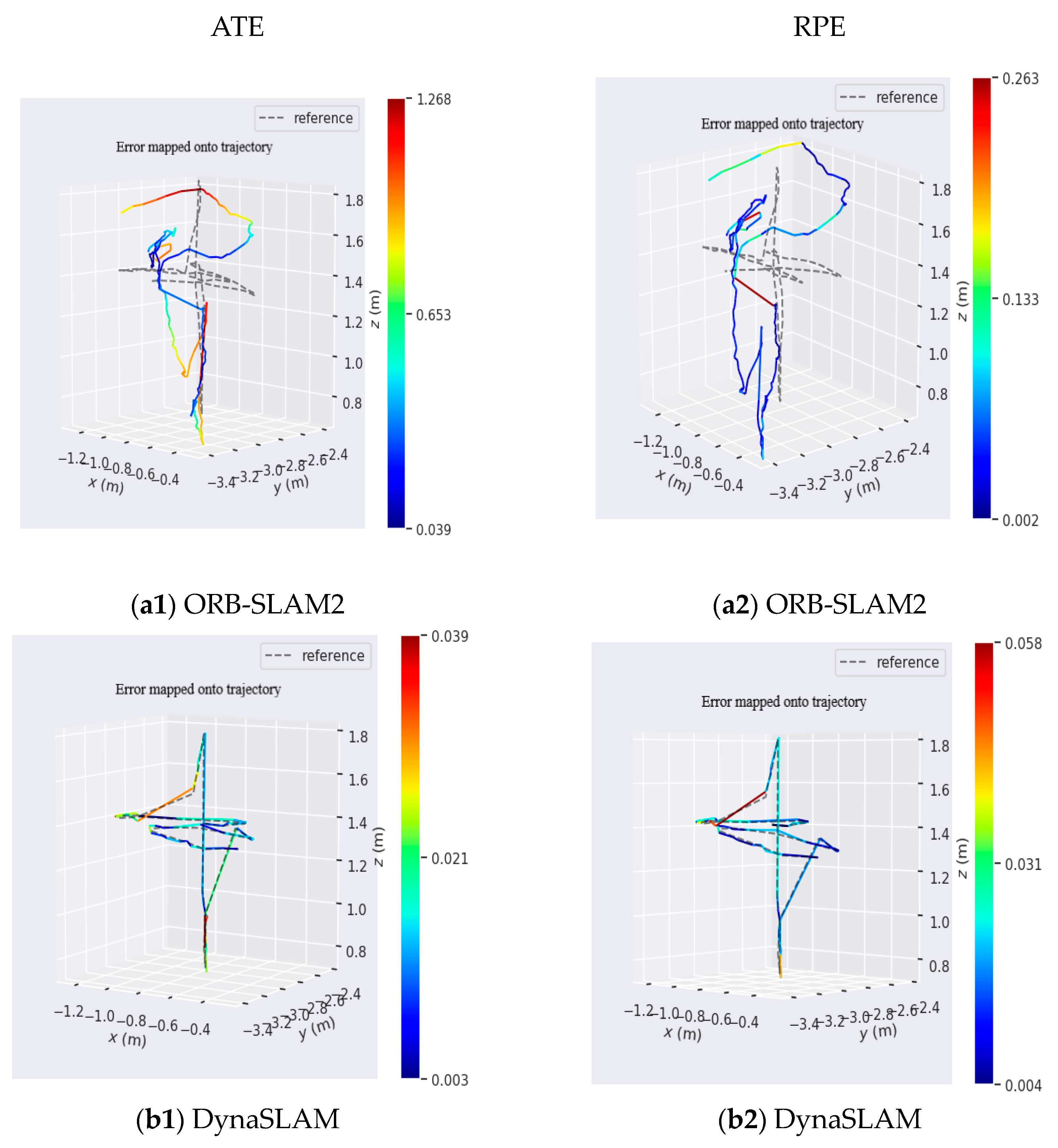
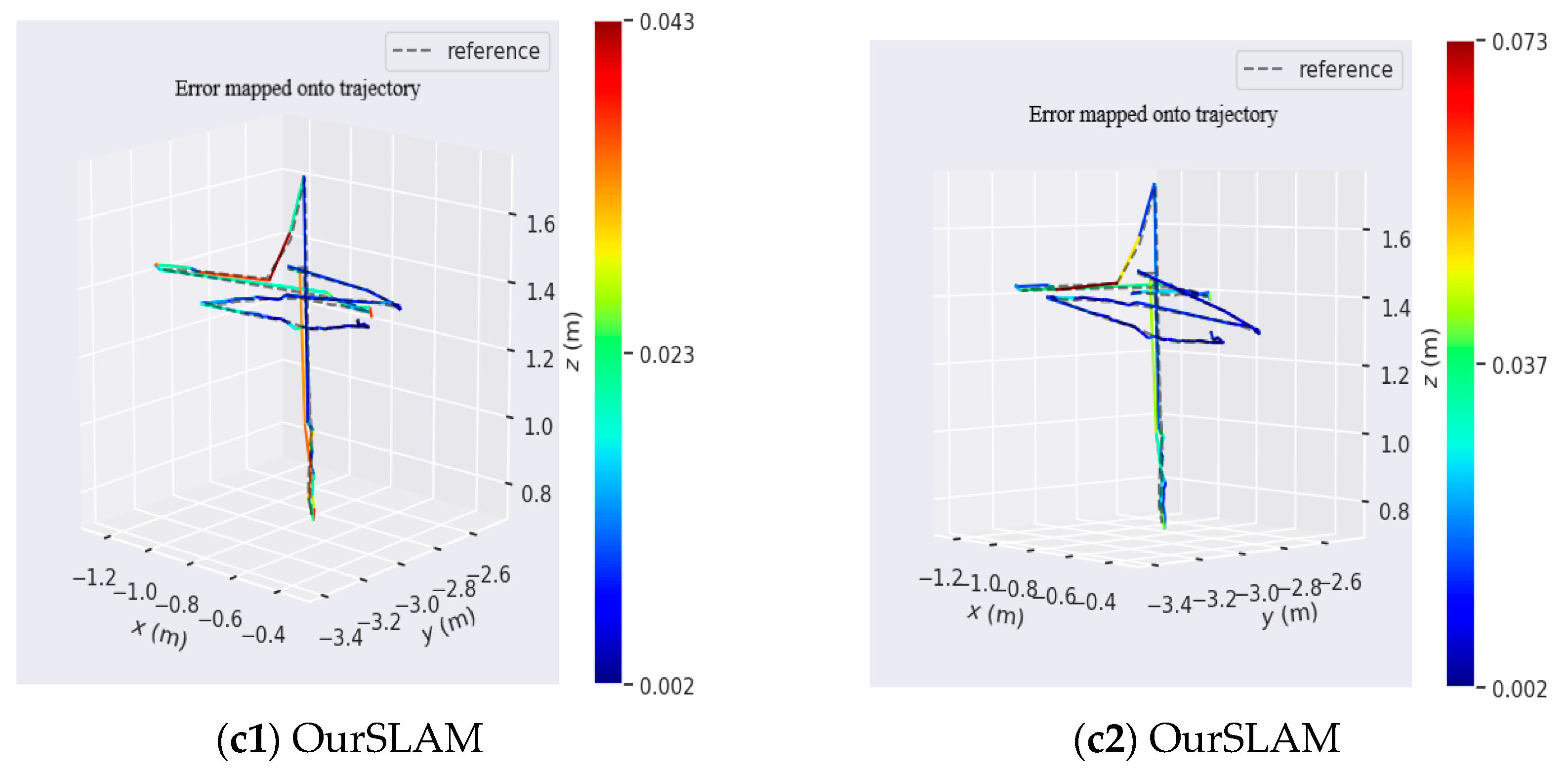
Figure 14 shows the ATE and RPE results of ORB-SLAM2, DynaSLAM, and OurSLAM algorithms running on the fr3_Warking_xyz dataset. The line segment on the right of the picture is the margin of error and the different colors are the allowable margin of error. Figure 14(a1,b1,c1) show the ATE results of fr3_Warking_xyz dataset running on three algorithms. The different colors in the diagram indicate the allowable margin of error, and there are roughly three ranges, blue, green, and red. Blue means the error is very small, within the allowable range; green indicates a large error, and red indicates a large error that is not within the allowable range. Figure 14(a1) shows the ATE operation result of ORB-SLAM2, in which the trajectory hardly coincides with the red line segment, indicating a very large error. Figure 14(b1) shows ATE results of DynaSLAM run under the fr3_Warking_xyz dataset. In Figure 14(b1), the DynaSLAM trajectory is consistent, with red line segments but a small error range. Figure 14(c1) shows the ATE result diagram of OurSLAM running under the fr3_Warking_xyz dataset. Figure 14(c1) shows that the trajectory is in good agreement without red line segments, indicating that the error is within the allowed range and the algorithm has high accuracy.

The algorithm proposed in this paper has obvious advantages in terms of operation speed compared with the DynaSLAM algorithm of the same type. The main reasons are as follows. In this paper, the lightweight YOLOv5 network improved by ShuffleNetV2 is used, which has a greater advantage in image processing speed compared with that of the Mask R-CNN network. The use of a multi-geometric approach to dynamic feature points in DynaSLAM is to detect objects that are likely to be in motion and objects that are in motion. This can lead to a long processing time and slow down the algorithm when dealing with image keyframes. For dynamic feature elimination, the potential moving objects and moving objects are deleted at the same time. This results in DynaSLAM deletion, long processing time per frame, and large pose estimation error. At the same time, DyanSLAM also adds background reconstruction, which uses the historical key frame of observation for background reconstruction, which generates a lot of redundant processing time in the algorithm and greatly reduces the running speed of the algorithm. The algorithm in this paper divides the dynamic objects in the environment into three parts: high dynamic, medium dynamic, and low dynamic, when processing dynamic features. An improved lightweight YOLOv5 network combined with geometric constraints was used for the joint detection of dynamic objects in the environment. First, the improved YOLOv5 network was used to detect dynamic objects in the environment, which were directly removed when they were in high and medium dynamic boxes. For those dynamic objects with prior static, the algorithm in this paper uses geometric constraints to eliminate them. Compared with the DynaSLAM algorithm, the algorithm in this paper requires less computation to deal with dynamic feature points and greatly improves the running speed. As DynaSLAM will delete potentially dynamic objects, it will result in large pose errors and low accuracy. This algorithm uses geometric constraints to identify and delete potentially dynamic objects, which improves the accuracy of camera pose estimation.

In the drawing construction of the SLAM system, the running speed and real-time performance of the system are also usually used as important indicators to evaluate the system. When verifying the running speed of the algorithm in this paper, the method of comparison is mainly used to verify the operation speed of the algorithm. In this paper, the time used for the keyframe processing of ORB-SLAM2, DynaSLAM, and OurSLAM algorithms is compared and analyzed to evaluate the running speed of these algorithms. The running results are shown in

Table 3. Real-time comparison of SLAM algorithms under a dynamic environment.

Datasets	Average Tracking Time per Frame/s
	OurSLAM	DynaSLAM	ORB-SLAM2
Warking_xyz	0.0601	1.127	0.0372
walking_halfsphere	0.0645	1.140	0.0379
walking_static	0.0632	1.152	0.0337
fr3_w_rpy	0.0636	1.138	0.0356
fr3_s_static	0.0658	1.153	0.0348

.

As shown in Table 3, OurSLAM and ORB-SLAM2 have little difference in the processing time of keyframes. Both of them can process key frames in a very short time. Therefore, the system runs fast and has good real-time performance during drawing construction. DynaSLAM has relatively long keyframe processing times. Therefore, the running time of the system will be relatively slow, with poor real-time performance, and prone to frame loss phenomenon.

5. Conclusions

Based on ORB-SLAM2, this paper uses the improved YOLOv5 network to build maps in dynamic environments, overcoming the drawbacks of low real-time performance and the poor robustness of SLAM systems in building maps in dynamic environments, and improving the accuracy of SLAM systems in building maps in dynamic environments as well as the real-time performance of the system in building maps. The algorithm in this paper improves the network based on the YOLOv5 network with a lightweight design and increases the operation speed of the network without reducing the network accuracy. The PSPNet semantic segmentation network is also added, making the improved YOLOv5 network capable of not only target detection but also semantic segmentation, which improves the accuracy of target detection. When building a SLAM system in a dynamic environment, the semantic information and geometric constraints can be used to reject dynamic objects in the environment more accurately, which improves the stability and quality of the SLAM system. Through experimental tests, the algorithm can obtain good results when building maps in dynamic environments, and it can meet the requirements of SLAM building in dynamic environments. In the future, we can consider combining with the multi-geometry view method to improve the stability of the system, so that the potential dynamic objects can be detected and rejected by the multi-geometry view method to improve the environmental adaptation performance of the system.