Review

A Systematic Review of Multi-Scale Spatio-Temporal Crime Prediction Methods

1
Public Safety Behavioral Science Lab, People’s Public Security University of China, Beijing 100038, China
2
College of Investigation, People’s Public Security University of China, Beijing 100038, China
*
Author to whom correspondence should be addressed.
ISPRS Int. J. Geo-Inf. 2023, 12(6), 209; https://doi.org/10.3390/ijgi12060209
Submission received: 27 February 2023 / Revised: 19 May 2023 / Accepted: 21 May 2023 / Published: 23 May 2023

Abstract

:
Crime is always one of the most important social problems, and it poses a great threat to public security and people. Accurate crime prediction can help the government, police, and citizens to carry out effective crime prevention measures. In this paper, the research on crime prediction is systematically reviewed from a variety of temporal and spatial perspectives. We describe the current state of crime prediction research from four perspectives (prediction content, crime types, methods, and evaluation) and focus on the prediction methods. According to various temporal and spatial scales, temporal crime prediction is divided into short-term prediction, medium-term prediction, and long-term prediction, and spatial crime prediction is divided into micro-, meso-, and macro-level prediction. Spatio-temporal crime prediction classification can be a permutation of temporal and spatial crime prediction classifications. A variety of crime prediction methods and evaluation metrics are also summarized, and different prediction methods and models are compared and evaluated. After sorting out the literature, it was found that there are still many limitations in the current research: (i) data sparsity is difficult to deal with effectively; (ii) the practicality, interpretability, and transparency of predictive models are insufficient; (iii) the evaluation system is relatively simple; and (iv) the research on decision-making application is lacking. In this regard, the following suggestions are proposed to solve the above problems: (i) the use of transformer learning technology to deal with sparse data; (ii) the introduction of model interpretation methods, such as Shapley additive explanations (SHAPs), to improve the interpretability of the models; (iii) the establishment of a set of standard evaluation systems for crime prediction at different scales to standardize data use and evaluation metrics; and (iv) the integration of reinforcement learning to achieve more accurate prediction while promoting the transformation of the application results.

1. Introduction

Crime is a continuous, dynamic, and complex process that is complexly related to time, space, and environment [1]. Most crimes, such as theft and robbery, are deeply connected to their spatial and temporal distribution. It has been proven that the spatial and temporal distribution of crime is not random, but rather exhibits a certain regularity and aggregation [2,3]. The places where the crimes occur are constantly concentrated, eventually forming “crime hotspots” [4,5]. Therefore, this makes crime prediction possible. Accurate and effective crime prediction has become an indispensable means of curbing and combating crime. It not only reduces the occurrence of crime, diminishes economic losses, and improves public safety, it also helps governments and police agencies to reasonably deploy police resources and improve allocation efficiency.
Crime prediction is mainly based on historical crime and environmental, socio-economic, and network social data, from which crime-related features are mined to predict the occurrence of crime in a certain spatial and temporal range in the future. This enables police departments to proactively allocate police resources and implement targeted prevention and control measures for a specific time and location, such as deploying scientific and reasonable patrol routes, determining the optimal patrol time, calculating the necessary number of patrols, and creating timely arrest plans. Based on this, many scholars have contributed substantially to the fields of crime prediction, crime hotspot mapping, and crime simulation, resulting in significant progress [6,7,8].
This paper focuses on crime prediction methods by analyzing the latest research on temporal and spatial crime prediction. The main work is as follows.
  • Studies related to crime prediction are systematically reviewed from various temporal and spatial perspectives.
  • Common temporal and spatial crime prediction methods and evaluation metrics are summarized.
  • The limitations of the current study are reviewed, and reasonable suggestions for future directions of exploration are provided.
The remaining structure of this review is organized as follows. In Section 2, the research methodology and an overview of the relevant studies are introduced. Section 3 introduces the common crime prediction methods and evaluation metrics. Section 4, Section 5 and Section 6 describe in detail the multi-scale temporal, spatial, and spatio-temporal crime prediction studies. Among them, temporal crime prediction is divided into short-term, medium-term, and long-term prediction; spatial crime prediction is divided into micro-, meso-, and macro-level prediction; and spatio-temporal crime prediction classification as a permutation of temporal and spatial crime prediction classifications, as shown in Figure 1. The last section concludes the paper and provides some suggestions for future work.

2. Materials and Methods

2.1. Publications Sources

This study followed the methods of collecting and screening literature that are in line with the preferred reporting items for systematic reviews and meta-analyses (PRISMA) guidelines [9] and conducted searches and screening of publications related to “spatio-temporal crime prediction” from 2013 to 2022.

2.1.1. Publications Search

To begin with, we searched for publications using the keywords (crime prediction, predict crime, crime forecasting, forecasting crime, spatio-temporal crime prediction, spatial crime prediction, and temporal crime prediction) in the bibliographic databases “Web of Science (WOS)”, “Institute of Electrical and Electronics Engineers (IEEE) Xplore”, “Association for Computing Machinery (ACM)”, and “China National Knowledge Internet (CNKI)”. A total of 12,579 publications were retrieved, including 7517 from the “WOS” database, 1087 from the “IEEE” database, 3723 from the “ACM” database, and 252 from the “CNKI” database. The latest search was conducted on 28 April 2023.

2.1.2. Publications Screening

In the next step, we removed the publications that that were duplicated, outside the scope of the publication types (conference, journal, and thesis), or without access and downloading permission. We then screened the remaining literature by reading the titles, abstracts, main bodies, and results to exclude those that were irrelevant to the topic, of poor quality, or of limited reference value. After screening, 79 publications remained, including 63 English-language publications and 16 Chinese-language publications.

2.2. Research Overview

After reading, summarizing, and organizing the selected publications, we sorted out the research on multiple spatio-temporal crime prediction methods according to four aspects: research content, prediction methods, types of crimes involved, and evaluation metrics. The overall profile of the crime prediction research is as follows.

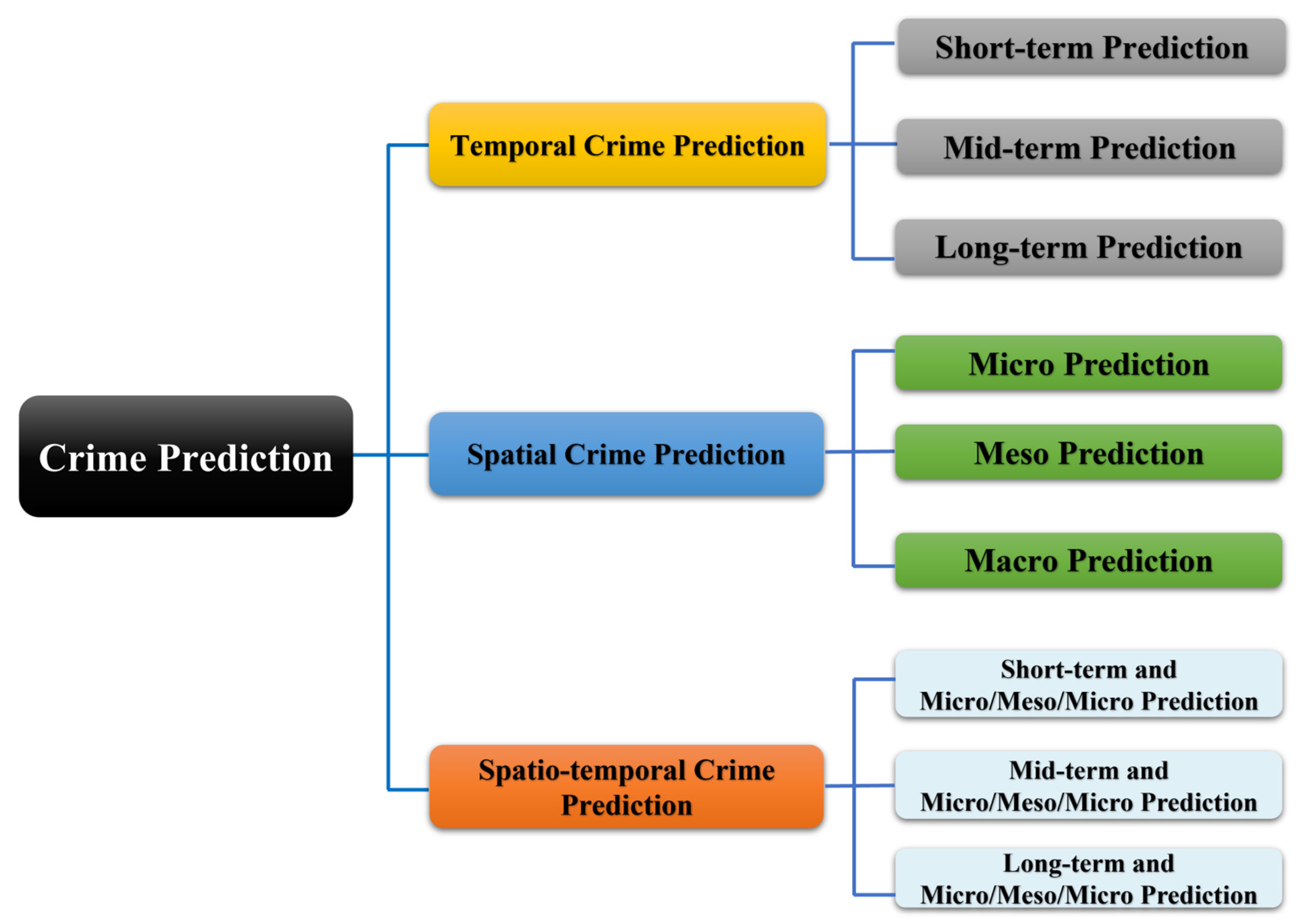
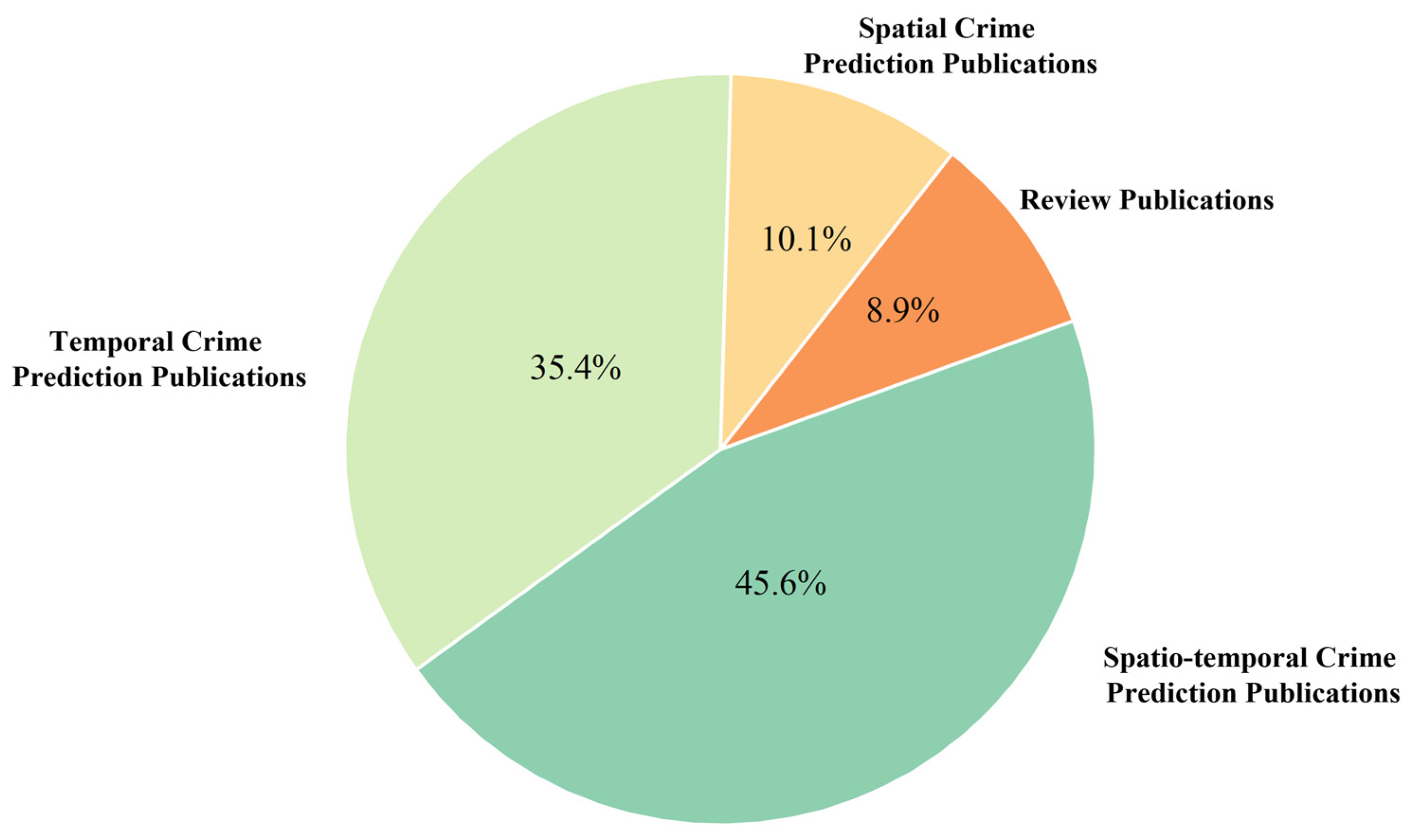
2.2.1. Research Content

Among the 79 selected publications, there were 7 review publications, 28 publications on temporal crime prediction, 8 publications on spatial crime prediction, and 36 publications on spatio-temporal crime prediction, as shown in Figure 2. Temporal crime prediction refers to predicting crime trends in a certain area over a future period, without considering crime hotspots or spatial distribution. Relatively speaking, the number of spatial crime prediction publications is small, which is due to the fact that most spatial crime prediction research generally combines specific time and crime types for analysis and prediction, which is then transformed into spatio-temporal crime prediction research.

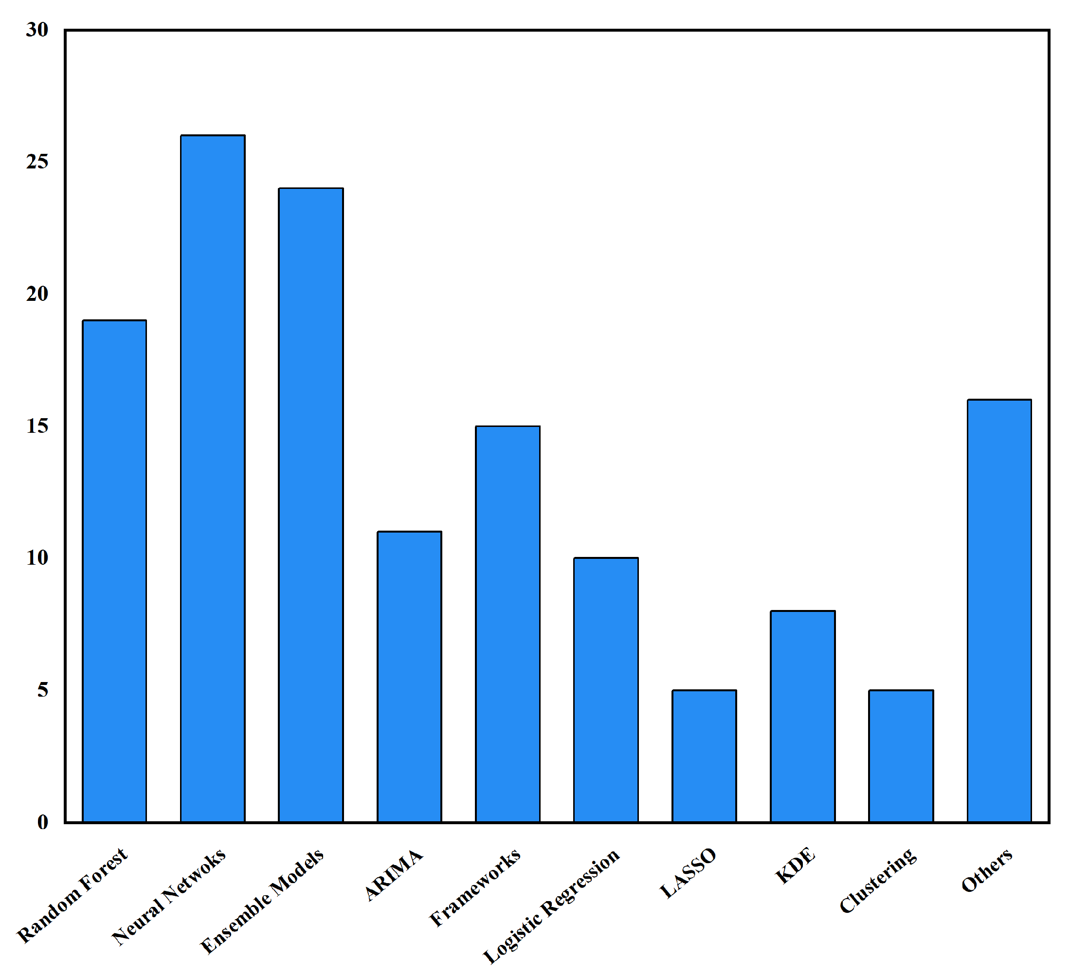
2.2.2. Prediction Methods

In terms of prediction methods, the most frequently used models and methods include neural network models (26 publications), ensemble learning models (24 publications, except for the random forest model), random forest models (19 publications), and various crime prediction frameworks (15 publications), as shown in Figure 3. Among them, ensemble, neural network, random forest, and autoregressive integrated moving average (ARIMA) models are commonly used for temporal crime prediction. Clustering, kernel density estimation (KDE), and risk terrain modeling (RTM) are commonly used for spatial crime prediction, and neural network, ensemble, and random forest models and various prediction frameworks are commonly used for spatio-temporal crime prediction. Additionally, the commonly used models for short-term crime prediction include the RF and LR models, as well as various crime prediction frameworks. Neural network models are often used for medium-term prediction. For long-term prediction, ARIMA and ensemble models are commonly used.

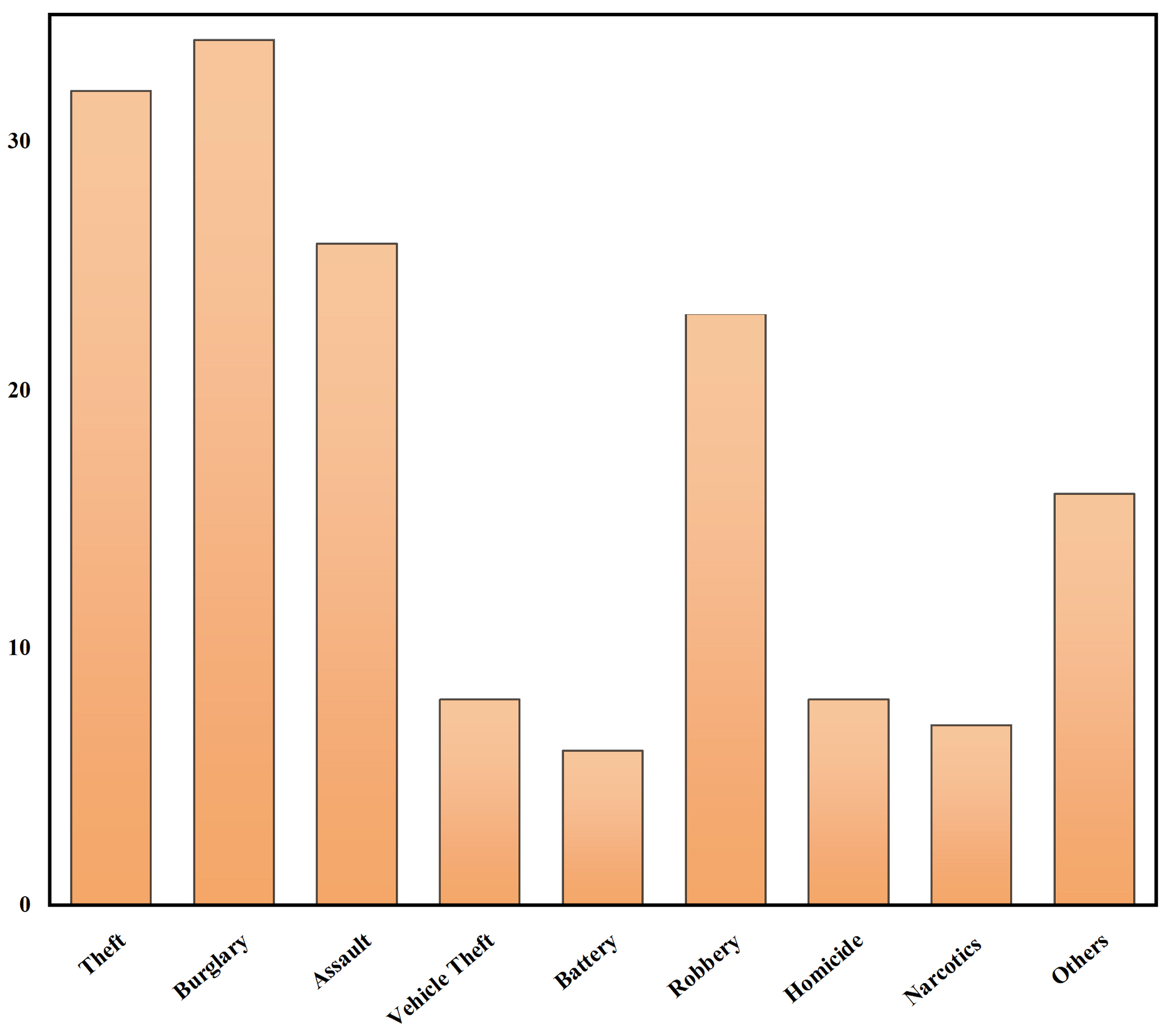
2.2.3. Types of Crime Predicted

As for the types of crimes predicted, common types include burglary (34 publications), theft (32 publications), assault (26 publications), robbery (23 publications), motor vehicle theft (8 publications), and homicide (8 publications), among others, as shown in Figure 4. On the one hand, there is a large quantity of crime data available for research purposes, which makes it easier to conduct crime prediction research. On the other hand, these types of crimes are closely related to daily life, making the related research more practical and meaningful. In addition, neural networks, ensemble models, and various frameworks are commonly used for assault and battery crime prediction. Neural networks, ensemble models, various frameworks, and ARIMA models are commonly used for theft crime prediction. Various frameworks, neural networks, ensemble learning, and RF models are commonly used for burglary crime prediction.

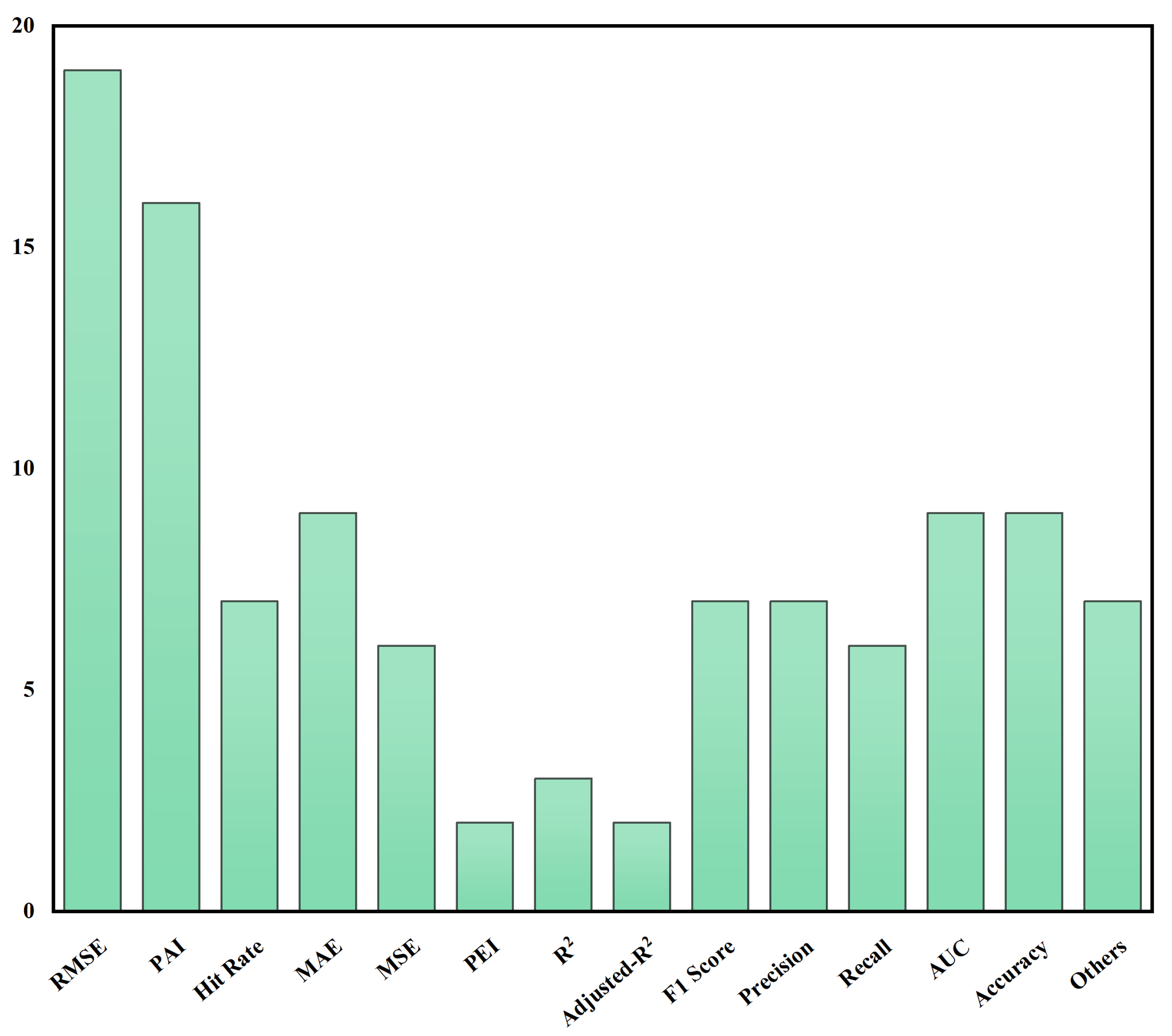
2.2.4. Evaluation Metrics

Evaluation metrics are the most important means of assessing model performance. From the publications, we compiled the top 5 evaluation metrics used in crime prediction research, including the root mean square error (RMSE, 19 publications), predictive accuracy index (PAI, 16 publications), mean absolute error (MAE, 9 publications), accuracy (9 publications), and area under curve (AUC, 9 publications), as shown in Figure 5. Among them, the RMSE, the mean square error (MSE) and accuracy are commonly used evaluation metrics for temporal crime prediction research. The PAI is commonly used for spatial crime prediction research, and RMSE and the PAI are commonly used for spatio-temporal crime prediction research. Therefore, in future crime research, RMSE can be selected as the main evaluation metric for temporal crime prediction, while the PAI can be selected as the main evaluation metric for spatial crime prediction. This is significant for comparing the prediction performance of various crime prediction methods.
In summary, we can describe the overall trend of existing crime prediction research in terms of prediction content, crime types, methods, and evaluation. Regarding research content, an increasing number of studies are focusing on spatio-temporal crime prediction. The types of crime predicted are mostly property crime (theft, burglary, and robbery) and violent crime (assault, battery, and homicide). As for prediction methods, increasingly complex ensemble models or frameworks designed to capture spatio-temporal characteristics of crime are being developed and used. In addition, while random forest models are also used frequently, this is partly because the random forest model is one of the effective machine learning models. With the development of machine learning, as many models and frameworks with better performance are being developed, random forest models are now more commonly used as baseline models. In terms of model evaluation, temporal crime prediction research generally uses RMSE and MSE to evaluate the models, while spatial crime prediction research commonly uses the PAI as an evaluation metric.

3. Crime Prediction Methods and Evaluation Metrics

3.1. Crime Prediction Methods

The methods commonly used for crime prediction can be divided into three categories: machine learning (ML), crime mapping, and other methods.

3.1.1. Machine Learning

In the past two decades, ML has made great strides in the fields of artificial intelligence (AI), biology, chemistry, materials science, agriculture, architecture, meteorology, natural language processing (NLP), and computer vision [10,11]. From face recognition, spam classification, and predicting house prices to driverless vehicles, ML is closely related to our daily lives. ML is a method of continuously training models with data so that the models grasp the potential laws embedded in the data, and then, these trained models can be used to classify, cluster, or predict new data, as shown in Figure 6. ML is broadly classified into supervised learning, unsupervised learning, and semi-supervised learning [12]. Among them, supervised learning mainly deals with classification and regression problems, while unsupervised learning focuses on solving problems such as clustering and association analysis. Semi-supervised learning is between supervised learning and unsupervised learning, and various goals such as classification, regression, and dimensionality reduction can be achieved through semi-supervised learning. Currently, the commonly used methods for crime prediction include LR, RF, ensemble algorithms, and neural networks.
(1)
Logistic Regression
LR is a classic and widely used classification algorithm. When using LR to deal with a binary classification problem, we can classify the dependent variable into positive and negative classifications, which are represented by 1 and 0, respectively. When the predicted value is higher than zero, the real value is taken as 1 and is judged to be a positive case. Conversely, the real value is taken as 0 and is judged to be a negative case. Additionally, LR needs to be classified by a sigmoid function. The function is used to map any independent variable to 1 , + 1 .
(2)
Random Forest
RF is a model based on the bagging algorithm and is also one of the most used ensemble algorithms for classification and regression. RF can be regarded as a collection of multiple decision trees that eventually form a forest. RF uses this forest to make predictions on new data and then calculates the number of votes for each prediction and uses the most voted for category as the final decision. As a result, RF has a higher prediction accuracy than individual decision tree models or other classification models. Moreover, RF can easily handle large amounts of high-dimensional data and is resistant to interference and simple to implement.
(3)
Ensemble Model
Regarding the problem of the poor accuracy of the decision tree model in dealing with complex data, ensemble algorithms can be adopted to improve the performance, such as bagging [13], gradient boosting (GB) [14], eXtreme gradient boosting (XGBoost) [15], and adaptive boost (AdaBoost).
(4)
Neural Networks
Neural networks are computational models that imitate the human neural system and are a crucial part of ML. They contain interconnected nodes mimicking human nerves that process inputs, recognize patterns, and classify tasks. They have been increasingly applied to crime prediction due to their high learning ability, good applicability and portability, and more accurate prediction results [16]. The main neural networks commonly used for crime prediction are the convolutional neural network (CNN), deep neural network (DNN) [17], recurrent neural network (RNN), graph convolution network (GCN), and long short-term memory (LSTM) [18].

3.1.2. Crime Mapping

Crime mapping has been widely used in police work for the past few decades. On the basis of identifying crime patterns and hotspots, utilizing crime mapping technology can predict potential locations for the occurrence of crime within a certain time and space range in the future and thus help police agencies to take preventive measures against crime in advance. Commonly used crime hotspot mapping methods are KDE and RTM [19].
(1)
KDE
KDE is a method used to visualize crime hotspots and predict crime. It works by generating a continuous, smooth surface map on a grid, which shows how crime density varies across the study area using all the crime data within the bandwidth (search radius). KDE can also be used to measure building density, predict stock risk, and detect crime hotspots [20]. Moreover, parameters such as grid cell size and bandwidth have a significant impact on the accuracy of KDE [21].
(2)
RTM
RTM is a geographic risk assessment method that is effective in identifying and predicting potential risk factors and their spatial impacts based on the characteristics of the landscape; it can then estimate the probability of crime occurring in the area at a micro-level [22]. By identifying and predicting crime locations, RTM can assist police agencies in developing targeted policing strategies and allocating limited policing resources to areas with a relatively higher risk. This approach can help to reduce the risk and occurrence of crime in the vicinity. RTM has been widely applied to a variety of crime types and has consistently achieved good results [23].
The theoretical background of RTM is mainly derived from environmental criminology [24]. Typically, there are many potential risk factors within an area, such as bars, stations, and grocery stores. RTM identifies these potential risk factors and assesses the crime risk in the area over a spatial and temporal scale, predicting where crime is likely to occur. Multiple landscape risk map layers are created and overlaid in a geographic information system (GIS) to generate a comprehensive risk terrain map. Rutgers University has developed risk terrain modeling diagnostic (RTMDx) software that can be used to diagnose and identify potential risk factors in high-crime areas [25]. In addition, RTM technology can be combined with KDE and combined analysis of case configurations (CACC) to significantly improve the accuracy and interpretability of the prediction [26].

3.1.3. Other Prediction Methods

In addition to the methods mentioned above, there are many models and techniques that have been utilized in crime prediction research and have achieved positive prediction results, such as ARIMA [27], least absolute shrinkage and selection operator (LASSO) [28], and agent-based modeling (ABM) [29].
(1)
ARIMA
ARIMA is commonly used for time series prediction, such as predicting the spread of COVID-19 on a global scale [30,31]. The ARIMA model consists of three components—auto regressive (AR), I, and moving average (MA), which are expressed as ARIMA (p, d, q), where p is the number of AR terms, d is the number of integrated terms, and q is the number of MA terms. Therefore, the ARIMA model can be regarded as a combination of the AR model and the MA model.
(2)
LASSO
LASSO regression is based on the least squares method, with an L1 regularization to prevent model overfitting and to improve generalization ability. LASSO regression has some advantages in estimating sparse models, and by making some indicator coefficients zero, the interpretability of the model can be improved. It is commonly used for screening variables and for risk analysis.
(3)
ABM
ABM is a modeling and simulation technique based on the simulation of individual behaviors. In ABM, each individual (agent) in the system is considered an autonomous entity with its own behavioral and decision-making rules which operates and interacts within its surrounding environment. By simulating each agent’s execution of these rules and observing their resulting behavior, ABM can be used to study many real-world issues, such as crime simulation. ABM can help us better understand and predict criminal behavior and can assist police and policymakers in devising better strategies and tools to fight and reduce crime.

3.2. Evaluation Metrics

Evaluating the effectiveness of the above models is a very important part of crime prediction research, and several metrics are typically used to measure the performance of different models.

3.2.1. Hit Rate

Hit rate is the simplest indicator to measure the performance of the crime prediction model.
h i t   r a t e = n N
where n denotes the number of predicted crimes in the hotspot area, and N denotes the total number of crimes in the prediction period.

3.2.2. PAI and PEI

The PAI is the hit rate of the predicted crime area relative to the whole study area [32]. The PAI is widely used to compare the accuracy and precision of KDE and RTM.
P A I = n N / a A
where a denotes the predicted crime hotspot area, and A denotes the total area of the study area.
The predictive efficiency index (PEI) is the ratio of the actual PAI to the assumed maximum PAI for a specific application scene.
P E I = P A I P A I m a x

3.2.3. Accuracy and F1 Score

Accuracy and the F1 score are commonly used performance measures for classification problems in machine learning. The confusion matrix consists of positive, negative, true, and false. Generally, a prediction category of 1 is positive; a prediction category of 0 is negative; a correct prediction is true; and an incorrect prediction is false.
There are four types of predicted outcomes for samples—true positive ( T P ), true negative ( T N ), false positive ( F P ), and false negative ( F N ). T P means that the sample is positive and is predicted to be positive. F P means that the sample is negative but is predicted to be positive. T N indicates that the sample is negative and is predicted to be negative. FN indicates that the sample is positive but is predicted to be negative.
Accuracy indicates the proportion of samples with the correct prediction results in the whole sample.
A c c u r a c y = T P + T N T P + T N + F P + F N
The F1 score is the harmonic average of precision and recall. Moreover, the larger the F1 score value, the better the prediction performance.
P r e c i s i o n = T P T P + F P
R e c a l l = T P T P + F N
F 1   score = 2 · P r e c i s i o n · R e c a l l R e c i s i o n + R e c a l l  
where P r e c i s i o n denotes the proportion of samples predicted to be positive relative to all the positive samples, and R e c a l l denotes the proportion of samples predicted to be positive relative to all the positive cases.

3.2.4. ROC and AUC

In the confusion matrix, there exist two critical indicators—true positive rate (TPR) and false positive rate (FPR). TPR measures the proportion of actual positives that are correctly identified by the model, while FPR measures the proportion of actual negatives that are incorrectly classified positive. They are a pair of contradictory performance metrics. To create a receiver operating characteristic (ROC) curve for a given machine learning model, one can plot the corresponding FPR and TPR at every possible threshold value on a two-dimensional coordinate plane. Connecting these points with a line produces the ROC curve, with FPR as the horizontal axis and TPR as the vertical axis. The ROC curve is a valuable tool for evaluating and comparing the accuracy of different models.
T P R = T P T P + F N
F P R = F N T N + F P
The AUC is the area under the ROC curve enclosed by the coordinate axis. Similarly, larger the AUC value, the better the prediction performance.

3.2.5. MSE and RMSE

The MSE and RMSE evaluate the performance of the model by measuring the degree of difference between the predicted and true values. In addition, similar evaluation metrics include MAE, mean relative error (MRE), and mean absolute percentage error (MAPE). The smaller the value of these indicators, the more stable the output of the model and the better its prediction performance.
M S E = 1 n i = 1 n ( y ^ i y i ) 2
R M S E = 1 n i = 1 n ( y ^ i y i ) 2
M A E = 1 n i = 1 n | y ^ i y i |
M A P E = 1 n i = 1 n y ^ i y i y i
where n is the number of samples, y ^ i is the predicted target value, and y i is the true value.

3.2.6. R2 and Adjusted R2

The R2 is a simple, easy-to-calculate, and intuitive correlation metric, which is generally used to evaluate the deviation between the predicted and true values of a regression model. The value of R2 ranges from 0 to 1. The closer the value is to 1, the better the fit of the model.
R 2 = 1 ( y ^ i y i ) 2 y i y ¯ 2
where n denotes the number of samples, y ^ i denotes the predicted value, y i denotes the true value, and y   ¯  denotes the mean value.
When the ratio of features number p to sample numbers n is more than 1:5, R2 will overestimate the actual fit. In this case, the choice of adjusted R2 can overcome the effect of the sample size on R2.
R a d j s u t e d 2 = 1 1 R 2 n 1 n p 1

4. Temporal Crime Prediction

Temporal crime prediction can be classified into three categories based on different time scales: short-term prediction, medium-term prediction, and long-term prediction. Short-term prediction is based on hours, days, and weeks, while medium-term prediction is based on months and quarters. Long-term prediction is typically based on years. Crime prediction techniques can be further classified based on the elements used for prediction. These methods may rely solely on crime data or may incorporate external data as well. A diagram illustrating the temporal crime prediction process is shown in Figure 7.

4.1. Temporal Crime Prediction Based on Crime Data Only

Police agencies have collected a large number of criminal records and stored them in crime databases. These data serve as the foundation for crime prediction studies, which typically include temporal information (time of crime, date of crime, etc.), spatial information (geographic location of crime, longitude, and latitude), and crime information (type of crime, number of crime incidents, etc.), as listed in Table 1. Analyzing these data helps in understanding the current crime situation, identifying high crime areas and patterns, and enabling targeted deployment of police resources. By adopting appropriate strategies to prevent and combat crimes in the future, crime prediction methods based on crime data can be used in short-term, medium-term, and long-term prediction analyses.

4.1.1. Short-Term Prediction

The literature presented a method based on SEPP and Green’s function, known as the data driven Green’s function (DDGF) model. This method can be used to predict the occurrence of ten different types of crime in Chicago for up to one week in advance [33]. In most cases, the DDGF method provided better predictions than the expectation-maximization (EM), prognostics and health management (PHM), and KDE methods.

4.1.2. Medium-Term and Long-Term Prediction

The main models for medium-term and long-term prediction are the STEP model, ARIMA model, ST-AR model, contextually biased matrix factorization (CBMF) model, and the spatial beta convergence model.
(1)
STEP
The literature presented the genetic fuzzy system STEP model, which was used to predict the crime rate in Tehran, Iran, over the following ten weeks [34]. The model was evaluated using both the simulated and real data of four crime types in Tehran. The method showed the best prediction performance when compared to four hotspot mapping techniques.
(2)
ARIMA
The literature used the ARIMA model to predict 14 categories of crime in England and Wales during the COVID-19 pandemic [35]. The study showed that the 12 categories of crime were lower than expected, except for anti-social behavior and drug offenses, which had higher than predicted actual values. This is mainly because the COVID-19 pandemic severely affected people’s mobility and social interactions, resulting in a dramatic change in crime over time. However, as restrictions were eased the crime rates began to gradually approach the expected levels. In another study, the literature utilized both a time series model (ARIMA) and a machine learning model (ANN) to predict the number of crimes in India over the following five years [36]. The modified ANN model had the best prediction accuracy with sufficient data. Conversely, the modified ARIMA model was the best.
(3)
ST-AR
The literature used the ST-AR model to predict violent crime and property crime rates over 15 years (1955–2009) for many countries and regions [37]. The results showed that the ST-AR model had the lowest RMSE compared to the other models, indicating that the model had the best predictive performance. Moreover, the model had a better prediction effect on property crime compared to violent crime.
(4)
CBMF
The literature transformed crime prediction into a recommendation problem and used the CBMF model to predict theft and assault in San Francisco [38]. The method was more efficient than traditional crime prediction methods, with 90.7% of burglaries and 79.6% of attacks captured using only 50% of the man-hours.
(5)
Spatial Beta Convergence
The literature presented a prediction model based on the beta convergence method [39]. The model was trained to predict homicide in 1120 inland cities of Colombia over the following 4 years. The results showed that the MAE and RMSE of the model were 1.55 and 2.35, respectively. Compared with the other four models, the MAE and RMSE decreased by an average of 0.33 and 0.56.

4.2. Temporal Crime Prediction Based on Crime and External Data

With the rapid development of the internet and smartphones, there are more and more fine-grained multi-source heterogeneous data, such as census, land use, point of interests (POIs), socio-economic, public service complaint, and meteorological data, as listed in Table 2.
The data contain a wealth of information on the spatial and temporal dynamics of crime and offer researchers the possibility to study the relationship between crime and demographics [40], housing, income, unemployment [41], education [42], economy [43], weather, climate [44], environment [45], social media [46], etc. For example, the literature studied the relationship between crime distribution and the land use data related to Szczecin, Poland [47]. The research showed that different types of land use have different effects on crime. Commercial buildings and dance halls tend to attract crime, while green areas and warehouses can inhibit the occurrence of crime. The study found that violent and property crime were strongly correlated with socio-economic factors and that racial heterogeneity was positively correlated with violent and property crime, while immigration, residential stability, and higher education were inversely correlated [48]. Many studies have shown that education level is negatively associated with crime, while unemployment has a positive effect on crime [49]. In addition, some researchers have studied the association of crime with social media [50], population mobility [51], air quality [52], green space [53], temperature [54], and road and street light density [55,56]. These data have great potential in crime analysis and prediction. Using data mining, data analytics, and other techniques, the data can be classified, collated, and analyzed; from this analysis, key features are extracted and input to various prediction models to determine the correlation between these factors and crime. Compared to methods solely based on crime data, combining crime and external data can significantly improve the accuracy of the predictions.

4.2.1. Short-Term Prediction

The models for short-term prediction include the localized kernel density estimation (LKDE) model, neural network models, ensemble models, and the neural attentive framework for hour-level crime prediction (NAHC).
(1)
LKDE
The literature analyzed the crime distribution of two sporting events (basketball and field hockey) and its correlation with Twitter data density [57]. They used historical crime data as the primary variables and social media with geo-tagged information, demographics, environment, and socio-economic data as covariates. These variables were selected as features using an RF classifier and then input into the LKDE model to make predictions for seven crime types on game days and non-game days, respectively. The study demonstrated that the social media data significantly improved the performance of the model compared with that based solely on crime data.
(2)
Neural Networks
The literature added census, weather, and public transportation data to the crime data to predict crime counts for three crime types (violent, burglary, and drug crimes) in Chicago and Portland using a combined CNN and RNN model [58]. In the model, the CNN model processed spatial features, and the RNN model processed temporal features. Firstly, Chicago and Portland were divided into multiple grid cells, each containing the corresponding features. Secondly, the CNN model was used to process the spatial features. Finally, the processing results and other features were input into the RNN model. On this basis, the importance of various variables was also verified. Compared with other neural network models, this model showed the best prediction performance, with an accuracy of 75.6% (Chicago) and 65.3% (Portland), respectively.
(3)
Ensemble Model
Ensemble models have been developed in the literature to predict the number of crimes and the level of crime risk, such the hybrid LSTM and GCN model, ST–GCN [59]. This framework consists of three modules: the spatio-temporal feature extraction, temporal feature extraction, and attention mechanism modules. Among them, LSTM was used for extracting temporal features; GCN was used for extracting spatial features; and self-attention was used for integrating spatio-temporal features and increasing the weight of important features. The model was used to predict the crime in Boston based on crime and meteorological data. The results showed that the R2 and RMSE were 0.84 and 2.30, respectively, in predicting burglary crimes on the scale of days, and the prediction performance was better than that of the LSTM and GCN models. The literature applied the ST–GCN model to predict burglary [60]. Firstly, a community topology map was constructed with each node containing crime, holiday, and weather data. Secondly, the temporal and spatio-temporal features were extracted using the LSTM and GCN modules, respectively. Crime change patterns and shift trends were captured using both modules. Finally, the predicted values of the two modules were combined using the gradient boosted decision tree (GBDT), from which the number of crimes in each community was predicted. Using this model to predict burglary in Chicago neighborhoods, the RMSE, MAPE, and R2 were 1.03, 0.39, and 0.84, respectively; these were lower than those of the ridge regression, LSTM, and RF models.
However, due to their “black-box” nature, ML-based crime prediction models are less transparent and explanatory, leading to weak interpretability and reliability. To address this limitation, an interpretable prediction model based on the XGBoost and SHAP was proposed in the literature [61]. This model predicts public theft at the XT police station with crime and environmental population data. The results showed that the accuracy of the XGBoost model was 0.89 and the ROC was 0.586. Additionally, the SHAP method was used to measure the contribution of each variable to the model to provide a reasonable interpretation of the results. The SHAP values were positively correlated with the variable’s contribution, indicating that non-local individuals aged 25 to 44 made a relatively large contribution to the model.
(4)
NAHC
Traditional models often struggle to capture spatio-temporal interactions between crimes occurring at different times and places. However, using the NAHC framework can effectively overcome this challenge and provide deeper insights into the spatio-temporal correlation of crime, resulting in more accurate crime prediction. The literature implemented hourly level crime prediction for Xiaogan City using the NAHC framework [62]. The crime situation at T + 1 can be predicted by the crime data at T and the external (POIs, meteorology, and environment) data at T and T + 1. The results demonstrated that the MSE of vehicle theft, assault, pickpocketing, and burglary were 0.0926, 0.0733, 0.0463, and 0.0246, respectively, indicating the excellent performance of the method.

4.2.2. Medium-Term Prediction

Medium-term prediction models usually include the latent Dirichlet allocation (LDA) model, DeepCrime framework, attention-based interpretable spatio-temporal network (AIST) framework, and integrated Laplace approximation (INLA) framework.
(1)
LDA
The LDA model was used to predict crime trends in Chicago over the following month [63]. The literature combined Twitter data and real data for 22 crime types to validate the model. It was found that adding temporal thematic features significantly contributed to improving the performance of the model, with an average improvement of 15%.
(2)
DeepCrime, AIST, and INLA
To better exploit crime-related spatio-temporal features, several studies presented frameworks that aimed to improve the performance and interpretability of crime prediction models. The literature developed DeepCrime, a deep neural network framework that embedded a hierarchical progressive framework to automatically capture crime dynamics over time and predict the monthly occurrence of four crime types (burglary, robbery, felony assault, and grand larceny) [64]. The F1 score of the model was higher than many machine learning algorithms. The literature proposed the AIST framework that captures the spatio-temporal correlation of crime to achieve monthly or quarterly level crime prediction [65]. The model was evaluated on a real dataset of four crime types (theft, criminal damage, battery, and narcotics) in Chicago, incorporating data such as public transportation and POIs. The result showed that AIST outperformed half of the baseline models. The literature designed an INLA framework for monthly level prediction of burglary in 20 neighborhoods of Amsterdam city [66]. This was a Bayesian spatio-temporal prediction framework that used burglary as the dependent variable of the study and land use, other crimes, and socio-economics served as covariates. The study found that, on the one hand, the closeness of the street network, the number of retail stores and street robberies were highly correlated with burglary. On the other hand, the study also demonstrated that the spatial and temporal distribution of burglary was concentrated.

4.2.3. Long-Term Prediction

Long-term prediction methods include the LASSO model, extremely randomized tree (extra trees) model, and ensemble models.
(1)
LASSO and Extra Trees
The literature explored the main factors influencing urban crime in China [67]. Homicide rates and six categories of urban indicators were used as features to train the models. Among them, the accuracy of the extra trees model (83%) was much higher than that of the LASSO model (51%). In addition, the importance of the relevant indicators was ranked. The results showed that the three most important factors influencing urban crime in China were the area of living land, the number of cell phone users, and the employed population.
(2)
Ensemble Model
The literature designed an instance-based transformer learning setup to address the problem of sparse data in small cities from a cross-domain perspective [68]. They incorporated 19 features from six different scenarios based on seasonal perspectives, such as crime, population, socio-economics, geographic location, and street lighting; these were used to train a GB classifier model to transform knowledge from different domains in Toronto and Vancouver (source domain) to Halifax (target domain). On this basis, the performance of the GB classifier, RF classifier, and other two transfer learning algorithms (TrAdaBoost and TrReasmpling) were evaluated using the AUC. The results showed that the GB classifier model had the best performance.
The literature utilized the RF, extra trees, and GB models for the long-term crime prediction of five felony types in New York City [69]. Three models were trained with census features, spatial features, and temporal features extracted from geo-tagged human mobility data. Among them, the extra trees model predicted the best performance. Furthermore, the model using human mobility data generally made better predictions than the model based on census data only. After introducing human mobility (socio-economics and public transportation) data, the average MSE of the models decreased by 0.22 and the average R2 increased by 15%. The literature used an RF regression model to predict the number of homicides in Brazil after 10 years, based on 13 indicators with 97% accuracy [70]. Moreover, the importance of urban indicators on homicide was identified, with unemployment, illiteracy, and male population being the three most important characteristics affecting this type of crime, while GDP was the least important one.

4.3. Limitations of Temporal Prediction Research

At present, the research on temporal crime prediction has a theoretical basis and a wealth of methodological advancements. Methodologically, the research has progressed from a single model to an integrated model and a deep learning framework, resulting in significantly improved prediction performance. In terms of data, the research has advanced from relying solely on crime data to using a combination of crime and external data to capture crime-related spatio-temporal characteristics, thereby improving prediction accuracy. However, current research still faces several deep-rooted problems that need to be addressed, such as ensuring the interpretability of the models, handling imbalanced data, and addressing ethical issues related to bias and privacy concerns.
  • Data sparsity. Despite the advancements in improving the accuracy of the models, most prediction models are driven by data and still have difficulties in dealing with data sparsity. Some study areas have limited crime data, making it challenging to support crime prediction. Furthermore, as the granularity of time and space becomes finer, the data become sparser and the amount of irrelevant information gradually increases, leading to difficulties in modeling crime. It also exposes issues regarding the difficulty involved in using data-driven models to accurately identify and extract crime-related features. Adding external features may result in reduced correlation between data and crime or even the phenomenon of the “Curse of Dimensionality”, where the model cannot converge quickly in a short time.
  • Insufficient practicality, interpretability, and transparency of the model. ML-based prediction models often lack interpretability due to their “black-box” nature. The improved performance of the model comes at the cost of interpretability. As the complexity of the model increases, its performance becomes stronger, but its interpretability becomes worse. It is not enough to evaluate a model based on accuracy alone; understanding the mechanics behind how the model works is crucial. It is important to know how prediction results are given and which features are crucial for the model, among other considerations. Otherwise, full trust in the prediction results cannot be established. Thus, there is a strong need to introduce model interpretability methods to improve the understanding of how the models function. Additionally, since the crime situation varies between regions, models trained in one region may not necessarily transfer well to other regions.
  • Single evaluation system. The evaluation metrics and data used in the above studies vary, making it impossible to judge the merits of the models accurately. Some studies rely solely on historical crime data, while others use a combination of crime and external data, such as demographic, socio-economic, and environmental factors. Moreover, the evaluation metrics are often too narrow, making it challenging to compare the performance of the models accurately. Thus, there is a need to establish a comprehensive evaluation system that considers various data types and evaluation metrics to truly judge the merit of the models.
  • Limited studies on short-term crime prediction. Most of the studies discussed above focus primarily on medium- and long-term crime prediction (monthly, quarterly, and annual), which has a positive impact on macro-level policy making. However, few studies concentrate on short-term prediction at the hourly, daily, and weekly levels. Short-term prediction better serves the needs of most police departments since crimes such as burglary and robbery are typically short-lived, and they require rapid action to prevent and combat the crimes effectively. The lack of research in short-term prediction models makes it difficult to prevent crime from happening, such as by deploying officers and planning patrol routes aimed at targeted areas. When an offense occurs, the perpetrators cannot be caught in time, resulting in a significant blow to law enforcement.

5. Spatial Crime Prediction

In spatial crime prediction, the predicted area is often divided into several grid units of different sizes, such as 150 m × 150 m or 200 m × 200 m. Typically, the larger the spatial unit, the higher the prediction accuracy [71]. However, grid cells that are too large are not aligned with the actual patrol range of police officers. Therefore, according to the analytic hierarchy process (AHP) method, crime spatial prediction can be divided into three levels: macro-, meso-, and micro-level predictions. Micro-level prediction mainly focuses on areas smaller than the existing functional zoning. Meso-level prediction mainly covers existing functional zoning, such as neighborhoods, communities, police districts, and census tracts. Macro-level prediction mainly involves predictions at the county, city, state, and national levels.

5.1. Micro- and Meso-Level Prediction

The micro- and meso-level spatial crime prediction pertains to community, campus, street, and rural area prediction, such as street robbery and community burglary. Crime patterns and crime levels in these areas vary significantly from those of other locations, and therefore, researchers have studied prediction in these geographical areas.
(1)
GLDNet
To address the problem of sparse urban street crime events, a graph-based deep learning framework—the grated localized diffusion network (GLDNet)—was proposed in the literature, and empirical research was conducted on three types of crimes in southern Chicago (assault, burglary, and theft) [72]. The results showed that, compared to the network-time kernel density estimation (NTKDE) method, GLDNet significantly improved the average hit rate, particularly in terms of 10% and 20% street length coverage rate; GLDNet improved by 12% and 25%, respectively.
(2)
Clustering
The literature utilized cluster analysis methods to detect hotspots of wildlife poaching in the Tsavo ecosystem (Kenya) [73]. Firstly, the study area was divided into 34 blocks. Then, spatio-temporal and spatial clustering methods were used to predict hotspots, and the PAI and the modified predictive index (MPAI) were introduced as evaluation metrics. The study showed that the predictive performances of spatial scan statistics (PAI = 2.39) and spatio-temporal scan statistics were better (MPAI = 1.46).
(3)
ANROC
The literature proposed an aggregated neighborhood risk of crime (ANROC) measure to enable a neighborhood-level prediction of violent crime rates [74]. They first used RTMDx to determine the best model and the community violent crime risk factors. Next, they constructed an ANROC to calculate the average risk value for each community unit. An ordinary least squares (OLS) regression model was used to predict violence in Little Rock, Arkansas, while controlling for centralized disadvantage and housing stability. The ANROC measure was significantly and positively correlated with community violent crime, suggesting that it helped to enhance the ability to understand changes in neighborhood violent crime and to achieve neighborhood-level violent crime predictions.
(4)
KDE and RTM
Using the street robbery data from Little Rock, Arkansas, the predictions were conducted, and the PAI and recapture index (RRI) were used to assess the techniques [75]. The study showed that the average PAI was highest for KDE (77.473), and the average RRI was highest for RTM (1.113) at all time scales. In other words, KDE had better prediction accuracy, while RTM had higher prediction precision.

5.2. Macro-Level Prediction

Accelerated urbanization has led to an influx of people, businesses, and industries into cities, which has increased the burden on urban areas and resulted in an upsurge in crime. Due to limited security resources, it is challenging for the police to respond to such a high volume of crime in a timely and effective manner. Hence, predicting urban crime has become critical to combatting the issue.
(1)
STDC Detector
To explore whether spatio-temporal crime geographical displacement (STCD) exists in China and whether utilizing the STCD detector can improve crime prediction accuracy [76], the literature studied burglary in a large Chinese city using the STCD detector and identified two important findings. Firstly, the existence of crime geographic displacement in China was confirmed, and the distances between displacements were not extensive. Secondly, utilizing an STCD detector increased the prediction accuracy, with improvements of 3.1% and 7.25% in the PAI and the capture rate, respectively. These results suggest the feasibility of the STCD detector in improving crime prediction.
(2)
RTM
Considering that the RTM technique ignores the dependence on successive events, the literature has generated four models (the random model, RTM-only model, event-dependent-only model, and integrated model) to predict the changes in crime distribution in large cities based on robbery data and land use data in Newark [77]. In all the models, the stochastic model showed the worst performance, while the integrated model had the best prediction. This suggests that combining event dependence and spatial influences can effectively improve the prediction of dynamic crime distributions.
(3)
ABM
The literature applied ABM to analyze crime patterns and prediction in a simulated environment [78]. ABM enabled agents to perceive their surroundings through the spatial, interactive, and temporal layers, helping them decide whether to engage in criminal activities. This integration of spatial, temporal, and interactive elements allowed the calculation of the probability of agents committing crimes and the prediction the next crime occurrence. Furthermore, the study conducted simulation experiments using data on robberies, points of interest (POIs), and weather in New York City. The results showed that the ABM model could accurately simulate crime patterns under varying environmental factors while providing valuable implications for the improvement of crime prediction.
This literature applied the agent-based model to simulate the behavior and interactions of criminals and police officers, with the aim of reducing crime rates through this model [29]. The agents in the model simulated the behavior of criminals and police officers, and the researchers investigated changes in different factors to understand the variation in crime rates. They also tested the effectiveness of the current policing strategies and adjusted their simulations according to the results obtained from the model. The study found that agent-based models could effectively evaluate and predict criminal behavior and provide valuable recommendations for anti-crime policies. Improving community development and implementing safety measures could reduce the likelihood of crime, while increasing the police presence or strengthening the surveillance of criminals could enhance the probability of apprehending them.
(4)
DNN Framework
Deep learning frameworks have demonstrated promising results in the prediction of crime hotspots. The literature [79] proposed three different configurations of deep learning frameworks in the literature; these are spatial features first then the temporal (SFTT); temporal features first then the spatial (TFTS); and spatial and temporal features in two parallel branches (ParB). Based on heterogeneous urban data sources (POIs, weather, demographics, etc.), ten advanced models and three configurations of deep learning models were trained. The results indicate that the SFTT model outperformed the other two configurations in terms of prediction performance. Additionally, the study identified the effectiveness of different parameters to facilitate the prediction of crime hotspots in urban areas. The study utilized machine learning, topic modeling, and sentiment analysis to identify and predict crime patterns and hotspots in Porto, Portugal [80]. Firstly, clustering analysis using the density-based spatial clustering of applications with noise (DBSCAN) algorithm was performed on the crime and census data. Then, machine learning methods were used to reveal feature correlations with crime. The study area was divided into multiple grid cells with a side length of 500 m to identify crime hotspots over the following year. Finally, LDA modeling and sentiment analysis were used to analyze Twitter data within a radius of 1 km from crime sites. The study showed that crime in Porto exhibited significant statistical, temporal, and spatial patterns, and the random forest algorithm had the best prediction performance. The emotional state reflected in tweets was closely related to crime locations.
The literature applied a data-driven approach to predict crime levels in the Greater London area [81]. By analyzing multiple heterogeneous datasets (crime, demographics, POIs, photographs, and land use data), more than 3000 features and 14 different crime types were selected. To enhance the robustness of the model, three regression algorithms (ridge regression, RF, and SVR) were selected as training models. Moreover, feature selection techniques were used to eliminate noise and improve the interpretability and accuracy of the model.

5.3. Limitations of Spatial Crime Prediction Research

  • Research on spatial crime prediction has made significant strides in identifying potential risk factors and crime hotspots, while also validating relevant criminology theories. However, despite the progress made thus far, this field still faces numerous challenges. For instance, the accuracy of crime prediction models heavily relies on the quality of crime data and the availability of relevant urban features. Moreover, the effective integration of various data sources remains a significant challenge in the development of reliable crime prediction models. There are fewer studies at the micro-level. While most studies in the spatial crime prediction field focus on macro-level predictions due to the availability of city-related data, they often overlook the importance of micro-level predictions. Conducting micro-level research would prove invaluable as it could assist the police in achieving scientific resource allocation and dispatch for specific areas and roads. Moreover, such research could enable enterprises to choose suitable business locations and to help citizens select safe travel routes and times, thus mitigating crime opportunities and promoting crime deterrence. The incorporation of micro-level predictions could provide more nuanced and context-specific insights and recommendations to a diverse group of stakeholders, thereby improving the effectiveness and efficiency of crime prevention strategies.
  • Lack of research on decision-making applications. Some studies lack practical support for assisted decision making, which impedes their practical applications. Going forward, there should be a stronger emphasis on the implementation of research results in assisting the development of scientific police decisions. For instance, integrating patrol route planning research and other decision-making tools would be valuable in optimizing crime prevention efforts. By bridging the gap between research and practice, stakeholders can more effectively employ spatial crime prediction models for actionable insights and evidence-based decision making.
  • Insufficient research on crime mechanisms. Although most spatial crime prediction studies successfully validate criminology-related theories and achieve the task of crime prediction to some extent, the directionality of some studies neglects the theoretical level. Consequently, these studies tend to only verify existing criminological theories, without sufficiently enriching or expanding the research on crime mechanisms. Additionally, the current research fails to consider the impact of criminal behavior patterns on crime prediction results. For instance, the presence of police on an offender’s travel route could deter the offender from committing the crime, which would subsequently affect the crime prediction accuracy. Therefore, future studies on spatial crime prediction should consider these contextual factors and aim to expand and advance crime mechanism research to improve the accuracy and applicability of crime prediction models.
  • Unreasonable grid cell size. Most spatial crime prediction studies employ grid cells with side lengths of 100 m, 150 m, and 200 m. The research indicates that larger grid sizes generally result in better prediction performance. However, the theoretical limit range of a police patrol is 150 m, which should be considered when considering the relationship between grid size and police patrol range in practical crime prediction and police work. Flexibly adjusting grid size according to actual conditions and police patrol frequencies is essential. For areas with frequent police patrol, smaller grid cells should be used for prediction and analysis to improve prediction accuracy, while for areas with insufficient police patrol, larger grid cells should be employed to maximize the use of limited police resources and ensure comprehensive coverage. Striking a balance between prediction performance and practical application is key in optimizing the implementation of spatial crime prediction models.

6. Spatio-Temporal Crime Prediction

The integration of temporal, spatial, and crime data not only helps to improve the accuracy of the predictions, it can also make the deployed prevention and control strategies more realistic. Due to the many possible permutations of temporal and spatial crime predictions, we provide a summary of the major spatio-temporal scales studied.

6.1. Short-Term and Micro-Level Prediction

The literature presented an improved deep spatio-temporal 3D convolutional neural network (ST3DNet) framework—ST3DNetCrime—for fine-scale (hourly and spatially small) crime prediction [82]. Using real data from Los Angeles for evaluation, the results showed that ST3DNetCrime had better prediction performance and robustness than the baseline models, especially ST3DNetCrime-f. This indicates that only by extracting all the spatio-temporal features from recent and near-historical crime data, as well as far-historical crime data, can the best prediction performance be achieved.

6.2. Short-Term and Meso-Level Prediction

The literature used the RF model to predict short-term (biweekly) crimes against property (robbery, snatching, and public theft) in public places to explore the influence of spatial variations and environmental variables on prediction results [83]. The study area (XT Street) was divided into 369 grids, each with a size of 150 m × 150 m, and the grids were clustered into four groups: stable high-incidence, high-incidence, occasional, and non-hotspot, based on their historical crime rates. Then, the RF model was constructed using only historical crime data or with the addition of environmental covariates (POIs, road network density, and urban villages), and control experiments were conducted. The results showed that spatial variations and environmental variables can improve the precision of prediction, especially in the stable high-incidence grids.

6.3. Short-Term and Macro-Level Prediction

The literature constructed different regression models based on crime data alone and combined crime and environmental data, respectively [84]. These models were used to predict residential and commercial break and entries (BNE) crimes in Vancouver, Canada. The prediction period was 1–30 days, the frequency was six times per day, and the distances were 500 m, 850 m, and 1 km. By visualizing the crime trends and spatial and temporal distributions of BNEs, the literature explored the relevant variables affecting such crimes. It was found that there was a spatial and temporal correlation between BNEs. Residential BNEs had higher recidivism rates within 850 m and 1 day from the last crime location, and commercial BNEs had higher recidivism rates beyond 500 m and within 2 days from the last crime location.
An “online” integrated graphical model based on attentional mechanisms was developed in the literature; it could extract and integrate spatio-temporal features, external features, and topological maps from crime data and achieve day-level urban crime prediction [85]. An empirical study using Chicago burglary and assault data found that the model was able to predict the spatio-temporal distribution of daily urban crime more accurately than the other models.
The study utilized the ST-Corking algorithm to detect the impact of potential offender activity on crime prediction [86]. Firstly, the study area was divided into 2604 grids (50 m × 50 m); then, a weekly, biweekly, and four-weekly crime prediction was made using historical crime data (theft and robbery) as the main variables and potential offender movement data as the covariates. The results showed that incorporating offender movement data could improve the prediction performance of the model, and the longer the duration of the prediction, the better the prediction performance.
The literature extracted temporal, spatial, and repeated crime features from various open-source data [87]. Then, a spatio-temporal crime model was constructed using a collaborative training model and a CoBayes model to infer road-level crime risk. The results demonstrated that the MAE of the model was 0.767, which was an average improvement of about 14.5% over the LASSO, LSTM, and SVR methods. Finally, an application capable of recommending the best risk-aware route was developed. This method was used to make an empirical study of New York City, and good results were achieved.
Based on the news feed data from Bangalore and India, the literature used the ARIMA and KDE models to predict the spatial and temporal distribution of crime over the following 15 days [88]. Firstly, the data related to crime were extracted from the news feeds using data mining techniques. Secondly, 68 crime types were classified into six categories based on keywords for identification and visualization of the crime distribution. Finally, the ARIMA model was used to predict the time series of crimes, and the KDE model was used to identify the hotspots. The results showed that the accuracy of the model was 75%, and most of the crimes were concentrated around the main places in the city. Among them, commercial crimes mostly occurred in Bangalore, and violent crimes were mostly concentrated in other parts of India.
Based on the data of public security, POIs, 311 public service complaints, meteorology, and population movement, the literature constructed a TCP framework, which could accurately capture the spatio-temporal correlation of urban data to predict the crimes in New York City over the following day and week [89]. Furthermore, the study identified the spatial distribution of crime over a week. In particular, the spatial distribution of crime was similar from Monday to Thursday, while Friday to Sunday had a similar spatial distribution of crime. Moreover, the crime distribution fluctuated the most on Friday, which meant that this day was the most unsafe.

6.4. Medium-Term and Macro-Level Prediction

The literature built models from different quarterly dimensions to predict four types of crime events in Salzburg, Austria [90]. Firstly, the risk factors associated with each type of crime event were identified with the help of RTMDx. Then, the results were entered into ArcGIS for testing. The study showed that the prediction results differed between crime events. Among them, assault had the highest prediction accuracy, and theft was predicted less well. Moreover, the possible reasons for these results were explained. The literature focused on the prediction of property crime (residential and vehicle theft) risk areas in economically developed cities. The impact of relevant risk factors on property crime in the city of Coral Gables was verified using the time dimensions of the day, week, month, and year, and its high-risk areas and relative-risk areas were explored and identified. The study found that the factors associated with auto and housing theft differed. Taken together, restaurants and grocery stores were common high-risk areas for both crimes.
The literature used an ensemble model based on logistic regression and neural networks to predict urban crime (home burglary, street robbery, and battery) trends over the following two weeks and one month [91]. It was shown that the monthly level prediction performance was significantly improved compared to the bi-weekly prediction, especially in predicting home burglary.
The literature developed a spatio-temporal kernel density estimation (STKDE) framework to predict crime hotspots by incorporating time components into the kernel density estimation (KDE) and conducted an empirical study on residential burglary in Baton Rouge [92]. The study used 100 m × 100 m grid cells as spatial units and predicted crime hotspots for the upcoming month, with a 1-week time-sliding window. The results showed that compared to spatial kernel density estimation (SKDE) and prospective hotspot mapping (ProMap), STKDE identified the most hotspots with the highest average PAI value. Furthermore, the method was capable of visualizing crime risks spatio-temporally.
Given the DNN models’ ability to automatically extract features, the literature utilized it to predict vehicle theft [93]. Vehicle theft data and 84 types of geographic data were used to train the DNN tuning model. The results showed that the DNN tuning model performed better than the RF, SVM, and KNN models.
The literature developed a deep learning framework—DeepPrison—which enabled burglary prediction at different granular levels [94]. The framework consisted of embedding and dense layers and a gated recurrent unit (GRU). It could extract burglary features and spatial and temporal features from historical crime data, socio-demographic data, and weather data and capture the potential correlations between various factors. By transforming burglary prediction into a binomial task, the model could achieve crime prediction within a specific region and time. On this basis, the model was evaluated using real datasets from Israel and New York City. The results demonstrated that the performance of DeepPrison was superior to the baseline models such as DeepCrime at all granularity levels.

6.5. Long-Term and Meso-Level Prediction

The paper validated the effectiveness of the Bayesian spatio-temporal modeling in analyzing crime trends and risks in small areas through the study of property crimes in the York region of Ontario, Canada in 2006 and 2007 [95]. The results demonstrated that the Bayesian spatio-temporal model can effectively predict property crime trends in small areas and identify crime hotspots and cold spots; this has practical implications for the deployment of law enforcement resources and the establishing of law enforcement plans.

6.6. Long-Term and Macro-Level Prediction

To solve the problem of crime data sparsity, the literature studied the influence of different population densities on crime prediction using hyper-ensemble models [96]. Taking burglary as an example, spatio-temporal features were assembled into 200 m × 200 m grid cells, and crime and weather features were also introduced. The prediction results exceeded the best baseline for each of the three different population density areas (low, medium, and high) tested. It was shown that the hyper-ensemble model had a very positive effect on offsetting the effect of crime sparsity. Based on this, combining the crime, location, and time features for the spatio-temporal prediction of low-density population areas can provide support for public decision making in low-population, imbalanced areas with sparse data.
The literature analyzed and predicted the spatio-temporal distribution and trends of urban crime by constructing a spatio-temporal Bayesian model and conducted an empirical study on residential burglary in Wuhan, China [97]. The results showed that residential burglary was positively correlated with the number of internet cafes and residential properties, as well as the unemployment rate, and residential burglary was mostly concentrated in the southern part of the Jianghan district. Therefore, internet cafes near these hotspots would be the focus of police patrols and inspections.
The literature used an ensemble model (GB) to predict the total number of crimes in 11 urban census tracts of the US, and the accuracy for violent and property crimes was 77% and 73%, respectively [98]. Based on criminology theory and crime correlation analysis, 118 predictive characteristics were selected from various data to predict the total number of crimes in urban and suburban areas over the following 5 years. Compared with the Poisson regression and deep learning models, the MAE of the GB model was reduced by 58.7 and 7.45, and R2 was improved by 45.8% and 4.1%.

6.7. Limitations of Spatio-Temporal Crime Prediction Research

On the one hand, spatio-temporal crime prediction effectively combines various time and space scales, making the research results more relevant to practical needs. On the other hand, this method of combination also exposes more complex problems related to time and space scales in research.
  • Spatio-temporal correlation. Crime is influenced by various factors, such as time, environment, weather, and networks, resulting in strong spatio-temporal correlations that make it difficult for traditional machine learning and time series analysis models to fully capture local or global spatio-temporal correlations. Blindly adding spatio-temporal crime data to some studies may lead to the overfitting of the model.
  • Spatio-temporal heterogeneity. The spatial and temporal distribution of crime is not uniform. Crime data in different times and regions often show differences, making it difficult for the same model to capture crime patterns in different times and regions simultaneously.
To address the spatio-temporal correlation and heterogeneity of crime, it is necessary to jointly model time and space, introduce self-supervised learning mechanisms, and design multi-task learning modules to achieve the functions of prediction, capturing spatio-temporal correlation and heterogeneity separately.

7. Conclusions and Future Perspectives

  • The continuous development of big data technology has enabled the use of advanced machine learning, hotspot mapping, and other methods for precise spatio-temporal crime prediction, resulting in significant progress and breakthroughs in this field. However, it is important to acknowledge that some prediction methods and techniques may not be able to fully address the complex and dynamic nature of contemporary crime. Thus, based on the literature review and analysis, this paper proposes reasonable and practical solutions to address the pressing issues and challenges in the research on spatial crime prediction. By addressing these challenges, we can further optimize and improve the efficiency and applicability of spatial crime prediction models in real-world settings. Data sparsity can be dealt with using transfer learning technologies. Data sparsity is a common challenge in the crime prediction field; it can limit the accuracy and generalizability of prediction models. The use of transfer learning techniques, a novel machine learning approach, offers a viable solution to this problem. Transfer learning allows the application of information and knowledge from existing domains to related domains, thereby enabling the training of deep learning models to capture connections between data and avoid overfitting, even with limited crime data. Additionally, when dealing with more data features and larger dimensions, feature selection, feature extraction, and cross-validation methods can be employed to optimize the performance and efficiency of spatial crime prediction models. By incorporating these techniques, researchers can more effectively address data sparsity issues and enhance the ability of spatial crime prediction models to capture and extrapolate meaningful patterns and trends.
  • Introducing model interpretability methods to improve the interpretability of models. Model interpretability is essential in enhancing the understanding and trustworthiness of prediction models. The issue of “black-box” models that produce predictions that are difficult to comprehend can be partially addressed by utilizing model interpretability methods, such as the LIME and SHAP models. LIME is a widely applicable model that facilitates both global and local interpretation of prediction results. On the other hand, the SHAP model considers all features as “contributors” and assigns SHAP values to each feature that are positively correlated with the contribution made by the variable. This approach enables the ranking of variables according to the SHAP value, thereby improving the interpretability of the model while retaining a high predictive performance. Incorporating model interpretability methods enhances our understanding of crime patterns and levels and enables the development of more scientific, accurate, timely, and effective prevention and control measures.
  • Establishing a set of data use and evaluation systems for multiple scales. A standard dataset usage and model evaluation system is crucial for crime prediction studies to promote accuracy, consistency, and interoperability. To this end, it is recommended to establish a set of data use and evaluation systems at each scale. Firstly, the standardization of the data use is essential to facilitate model comparison and ensure that models with the same prediction objectives and requirements employ the same type of dataset. Secondly, developing a comprehensive evaluation system is vital to facilitate the accurate performance measurement of such models. Using consistent evaluation metrics for models with the same prediction objectives is critical in gauging the efficacy of different models and developing a cross-comparable model evaluation framework. By incorporating these measures, we can establish a standard data usage and model evaluation system that promotes the accuracy, validity, and practical viability of crime prediction models at multiple scales.
  • Integrating other technologies to promote research in decision making. To address the current issues of low correlation between spatio-temporal crime prediction models and lack of targeted prevention and control strategies, innovative technologies such as crime simulation and reinforcement learning can be incorporated to enhance decision-making applications. With further advancements in crime simulation and reinforcement learning technologies, we can enhance the decision-making applications in the spatial crime prediction field and develop effective prevention and control strategies to combat crime more efficiently. Integrating spatio-temporal elements into a crime simulation model can provide a comprehensive approach to spatial crime prediction. Through crime simulation, the potential time and place of crime occurrences can be predicted, and the process of crime can be visually presented. Such information can be input into a deep reinforcement learning framework to optimize crime prevention and control strategies through a continuous learning process. The deep reinforcement learning (DRL) crime prevention and control strategy optimization model continuously learns and evaluates strategies for a wide range of crime scenarios, while selecting the optimal strategy for resource allocation in specific spatio-temporal environments [99,100]. Police agencies can utilize the reinforcement learning strategy selection mechanism to deploy police resources, develop patrol plans, and implement arrest operations effectively. In addition, this approach can also enable prompt apprehension of perpetrators and can minimize losses in the event of a crime occurrence. By combining simulation modeling, deep reinforcement learning, and crime prevention strategies, we can enhance the implementation and effectiveness of spatial crime prediction models, contributing to more efficient and targeted crime prevention and control measures.

Author Contributions

Yingjie Du, data curation, writing—original draft preparation; Ning Ding, conceptualization, methodology, supervision, writing—review and editing. All authors have read and agreed to the published version of the manuscript.

Funding

This research was funded by the Public Security First-class Discipline Cultivation and Public Safety Behavioral Science Lab Project (No. 2023ZB02) and the National Key R&D Program of China (No. 2020YFC1522600).

Data Availability Statement

No new data were created or analyzed in this study. Data sharing is not applicable to this article.

Conflicts of Interest

The authors declare that they have no known competing financial interests or personal relationships that could have appeared to influence the work reported in this paper.

References

  1. Malleson, N. Using agent-based models to simulate crime. In Agent-Based Models of Geographical Systems; Springer: Dordrecht, The Netherlands, 2011; pp. 411–434. [Google Scholar] [CrossRef]
  2. Brantingham, P.L.; Brantingham, P.J. Mobility, Notoriety, and Crime: A Study in the Crime Patterns of Urban Nodal Points. J. Environ. Syst. 1981, 11, 89–99. [Google Scholar] [CrossRef]
  3. Weisburd, D. The law of crime concentration and the criminology of place. Criminology 2015, 53, 133–157. [Google Scholar] [CrossRef]
  4. Curman, A.S.N.; Andresen, M.A.; Brantingham, P.J. Crime and Place: A Longitudinal Examination of Street Segment Patterns in Vancouver, BC. J. Quant. Criminol. 2015, 31, 127–147. [Google Scholar] [CrossRef]
  5. Ratcliffe, J.H. Crime Mapping and the Training Needs of Law Enforcement. Eur. J. Crim. Policy Res. 2002, 10, 65–83. [Google Scholar] [CrossRef]
  6. Wang, Q.; Jin, G.; Zhao, X.; Feng, Y.; Huang, J. CSAN: A neural network benchmark model for crime forecasting in spatio-temporal scale. Knowl.-Based Syst. 2020, 189, 105120. [Google Scholar] [CrossRef]
  7. Weisburd, D.; Braga, A.A.; Groff, E.R.; Wooditch, A. Can hot spots policing reduce crime in urban areas? An agent-based simulation. Criminology 2017, 55, 137–173. [Google Scholar] [CrossRef]
  8. Zhu, H.; Wang, F. An agent-based model for simulating urban crime with improved daily routines. Comput. Environ. Urban Syst. 2021, 89, 101680. [Google Scholar] [CrossRef]
  9. Liberati, A.; Altman, D.G.; Tetzlaff, J.; Mulrow, C.; Gøtzsche, P.C.; Ioannidis, J.P.; Clarke, M.; Devereaux, P.J.; Kleijnen, J.; Moher, D. The PRISMA Statement for Reporting Systematic Reviews and Meta-Analyses of Studies That Evaluate Health Care Interventions: Explanation and Elaboration. Ann. Intern. Med. 2009, 151, W65–W94. [Google Scholar] [CrossRef]
  10. Jordan, M.I.; Mitchell, T.M. Machine learning: Trends, perspectives, and prospects. Science 2015, 349, 255–260. [Google Scholar] [CrossRef]
  11. Liakos, K.G.; Busato, P.; Moshou, D.; Pearson, S.; Bochtis, D. Machine learning in agriculture: A review. Sensors 2018, 18, 2674. [Google Scholar] [CrossRef]
  12. Brunton, S.L.; Noack, B.R.; Koumoutsakos, P. Machine learning for fluid mechanics. Annu. Rev. Fluid Mech. 2020, 52, 477–508. [Google Scholar] [CrossRef]
  13. Bühlmann, P. Bagging, boosting and ensemble methods. In Handbook of Computational Statistics; Springer: Berlin/Heidelberg, Germany, 2012; pp. 985–1022. [Google Scholar]
  14. Bentéjac, C.; Csörgő, A.; Martínez-Muñoz, G. A comparative analysis of gradient boosting algorithms. Artif. Intell. Rev. 2020, 54, 1937–1967. [Google Scholar] [CrossRef]
  15. Song, K.; Yan, F.; Ding, T.; Gao, L.; Lu, S. A steel property optimization model based on the XGBoost algorithm and improved PSO. Comput. Mater. Sci. 2019, 174, 109472. [Google Scholar] [CrossRef]
  16. Wang, B.; Zhang, D.; Zhang, D.; Brantingham, P.J.; Bertozzi, A.L. Deep learning for real time crime forecasting. arXiv 2017, arXiv:1707.03340. [Google Scholar] [CrossRef]
  17. Kang, H.-W.; Kang, H.-B. Prediction of crime occurrence from multi-modal data using deep learning. PLoS ONE 2017, 12, e0176244. [Google Scholar] [CrossRef] [PubMed]
  18. Dong, Q.; Ye, R.; Li, G. Crime amount prediction based on 2D convolution and long short-term memory neural network. ETRI J. 2022, 44, 208–219. [Google Scholar] [CrossRef]
  19. Andresen, M.A.; Hodgkinson, T. Predicting Property Crime Risk: An Application of Risk Terrain Modeling in Vancouver, Canada. Eur. J. Crim. Policy Res. 2018, 24, 373–392. [Google Scholar] [CrossRef]
  20. Boppuru, P.R.; Ramesha, K. Geo-Spatial Crime Analysis Using Newsfeed Data in Indian Context. Int. J. Web-Based Learn. Teach. Technol. 2019, 14, 49–64. [Google Scholar] [CrossRef]
  21. Hart, T.; Zandbergen, P. Kernel density estimation and hotspot mapping: Examining the influence of interpolation method, grid cell size, and bandwidth on crime forecasting. Polic. Int. J. 2014, 37, 305–323. [Google Scholar] [CrossRef]
  22. Caplan, J.M.; Kennedy, L.W.; Miller, J. Risk Terrain Modeling: Brokering Criminological Theory and GIS Methods for Crime Forecasting. Justice Q. 2011, 28, 360–381. [Google Scholar] [CrossRef]
  23. Marchment, Z.; Gill, P. Systematic review and meta-analysis of risk terrain modelling (RTM) as a spatial forecasting method. Crime Sci. 2021, 10, 12. [Google Scholar] [CrossRef]
  24. Brantingham, P.; Brantingham, P. Criminality of place. Eur. J. Crim. Policy Res. 1995, 3, 5–26. [Google Scholar] [CrossRef]
  25. Kennedy, L.W.; Caplan, J.M.; Piza, E. Risk Clusters, Hotspots, and Spatial Intelligence: Risk Terrain Modeling as an Algorithm for Police Resource Allocation Strategies. J. Quant. Criminol. 2010, 27, 339–362. [Google Scholar] [CrossRef]
  26. Drawve, G.; Grubb, J.; Steinman, H.; Belongie, M. Enhancing Data-Driven Law Enforcement Efforts: Exploring how Risk Terrain Modeling and Conjunctive Analysis Fit in a Crime and Traffic Safety Framework. Am. J. Crim. Justice 2018, 44, 106–124. [Google Scholar] [CrossRef]
  27. Islam, K.; Raza, A. Forecasting crime using ARIMA model. arXiv 2020, arXiv:2003.08006. [Google Scholar] [CrossRef]
  28. Nitta, G.R.; Rao, B.Y.; Sravani, T.; Ramakrishiah, N.; BalaAnand, M. LASSO-based feature selection and naïve Bayes classifier for crime prediction and its type. Serv. Oriented Comput. Appl. 2019, 13, 187–197. [Google Scholar] [CrossRef]
  29. Malleson, N.; Heppenstall, A.; See, L. Crime reduction through simulation: An agent-based model of burglary. Comput. Environ. Urban Syst. 2010, 34, 236–250. [Google Scholar] [CrossRef]
  30. Swaraj, A.; Verma, K.; Kaur, A.; Singh, G.; Kumar, A.; de Sales, L.M. Implementation of stacking based ARIMA model for prediction of COVID-19 cases in India. J. Biomed. Inform. 2021, 121, 103887. [Google Scholar] [CrossRef]
  31. Alabdulrazzaq, H.; Alenezi, M.N.; Rawajfih, Y.; Alghannam, B.A.; Al-Hassan, A.A.; Al-Anzi, F.S. On the accuracy of ARIMA based prediction of COVID-19 spread. Results Phys. 2021, 27, 104509. [Google Scholar] [CrossRef]
  32. Chainey, S.; Tompson, L.; Uhlig, S. The Utility of Hotspot Mapping for Predicting Spatial Patterns of Crime. Secur. J. 2008, 21, 4–28. [Google Scholar] [CrossRef]
  33. Kajita, M.; Kajita, S. Crime prediction by data-driven Green’s function method. Int. J. Forecast. 2019, 36, 480–488. [Google Scholar] [CrossRef]
  34. Farjami, Y.; Abdi, K. A genetic-fuzzy algorithm for spatio-temporal crime prediction. J. Ambient. Intell. Humaniz. Comput. 2021, 1–13. [Google Scholar] [CrossRef]
  35. Langton, S.; Dixon, A.; Farrell, G. Six months in: Pandemic crime trends in England and Wales. Crime Sci. 2021, 10, 6. [Google Scholar] [CrossRef]
  36. Jha, S.; Yang, E.; Almagrabi, A.O.; Bashir, A.K.; Joshi, G.P. RETRACTED ARTICLE: Comparative analysis of time series model and machine testing systems for crime forecasting. Neural Comput. Appl. 2020, 33, 10621–10636. [Google Scholar] [CrossRef]
  37. Shoesmith, G.L. Space–time autoregressive models and forecasting national, regional and state crime rates. Int. J. Forecast. 2013, 29, 191–201. [Google Scholar] [CrossRef]
  38. Zhang, Y.; Siriaraya, P.; Kawai, Y.; Jatowt, A. Predicting time and location of future crimes with recommendation methods. Knowl.-Based Syst. 2020, 210, 106503. [Google Scholar] [CrossRef]
  39. Santos-Marquez, F. Spatial beta-convergence forecasting models: Evidence from municipal homicide rates in Colombia. J. Forecast. 2021, 41, 294–302. [Google Scholar] [CrossRef]
  40. Boivin, R. Routine activity, population(s) and crime: Spatial heterogeneity and conflicting Propositions about the neighborhood crime-population link. Appl. Geogr. 2018, 95, 79–87. [Google Scholar] [CrossRef]
  41. Altindag, D.T. Crime and unemployment: Evidence from Europe. Int. Rev. Law Econ. 2012, 32, 145–157. [Google Scholar] [CrossRef]
  42. Groot, W.; Brink, H.M.V.D. The effects of education on crime. Appl. Econ. 2010, 42, 279–289. [Google Scholar] [CrossRef]
  43. Jonathan, O.E.; Olusola, A.J.; Bernadin, T.C.A.; Inoussa, T.M. Impacts of Crime on Socio-Economic Development. Mediterr. J. Soc. Sci. 2021, 12, 71. [Google Scholar] [CrossRef]
  44. Ranson, M. Crime, weather, and climate change. J. Environ. Econ. Manag. 2014, 67, 274–302. [Google Scholar] [CrossRef]
  45. Inlow, A.R. A comprehensive review of quantitative research on crime, the built environment, land use, and physical geography. Sociol. Compass 2021, 15, e12889. [Google Scholar] [CrossRef]
  46. Vo, T.; Sharma, R.; Kumar, R.; Son, L.H.; Pham, B.T.; Bui, D.T.; Priyadarshini, I.; Sarkar, M.; Le, T. Crime rate detection using social media of different crime locations and Twitter part-of-speech tagger with Brown clustering. J. Intell. Fuzzy Syst. 2020, 38, 4287–4299. [Google Scholar] [CrossRef]
  47. Sypion-Dutkowska, N.; Leitner, M. Land Use Influencing the Spatial Distribution of Urban Crime: A Case Study of Szczecin, Poland. ISPRS Int. J. Geo-Inf. 2017, 6, 74. [Google Scholar] [CrossRef]
  48. Clancy, K.; Chudzik, J.; Snowden, A.J.; Guha, S. Reconciling data-driven crime analysis with human-centered algorithms. Cities 2022, 124, 103604. [Google Scholar] [CrossRef]
  49. Andresen, M.A. Unemployment, GDP, and Crime: The Importance of Multiple Measurements of the Economy. Can. J. Criminol. Crim. Justice 2015, 57, 35–58. [Google Scholar] [CrossRef]
  50. Hipp, J.R.; Bates, C.; Lichman, M.; Smyth, P. Using Social Media to Measure Temporal Ambient Population: Does it Help Explain Local Crime Rates? Justice Q. 2019, 36, 718–748. [Google Scholar] [CrossRef]
  51. Gerell, M. Does the Association Between Flows of People and Crime Differ Across Crime Types in Sweden? Eur. J. Crim. Policy Res. 2021, 27, 433–449. [Google Scholar] [CrossRef]
  52. Ding, N.; Zhai, Y. Crime prevention of bus pickpocketing in Beijing, China: Does air quality affect crime? Secur. J. 2019, 34, 262–277. [Google Scholar] [CrossRef]
  53. Venter, Z.S.; Shackleton, C.; Faull, A.; Lancaster, L.; Breetzke, G.; Edelstein, I. Is green space associated with reduced crime? A national-scale study from the Global South. Sci. Total. Environ. 2022, 825, 154005. [Google Scholar] [CrossRef] [PubMed]
  54. Hou, K.; Zhang, L.; Xu, X.; Yang, F.; Chen, B.; Hu, W.; Shu, R. High ambient temperatures are associated with urban crime risk in Chicago. Sci. Total. Environ. 2023, 856, 158846. [Google Scholar] [CrossRef]
  55. Ye, C.; Chen, Y.; Li, J. Investigating the Influences of Tree Coverage and Road Density on Property Crime. ISPRS Int. J. Geo-Inf. 2018, 7, 101. [Google Scholar] [CrossRef]
  56. Xu, Y.; Fu, C.; Kennedy, E.; Jiang, S.; Owusu-Agyemang, S. The impact of street lights on spatial-temporal patterns of crime in Detroit, Michigan. Cities 2018, 79, 45–52. [Google Scholar] [CrossRef]
  57. Ristea, A.; Al Boni, M.; Resch, B.; Gerber, M.S.; Leitner, M. Spatial crime distribution and prediction for sporting events using social media. Int. J. Geogr. Inf. Sci. 2020, 34, 1708–1739. [Google Scholar] [CrossRef]
  58. Stec, A.; Klabjan, D. Forecasting crime with deep learning. arXiv 2018, arXiv:1806.01486. [Google Scholar] [CrossRef]
  59. Hu, J. A Hybrid GCN and LSTM Structure Based on Attention Mechanism for Crime Prediction. Converter 2021, 328–338. [Google Scholar] [CrossRef]
  60. Han, X.; Hu, X.; Wu, H.; Shen, B.; Wu, J. Risk Prediction of Theft Crimes in Urban Communities: An Integrated Model of LSTM and ST-GCN. IEEE Access 2020, 8, 217222–217230. [Google Scholar] [CrossRef]
  61. Liang, X.; Liu, X.; Lan, M.; Song, G.; Xiao, L.; Chen, J. Interpretable machine learning models for crime prediction. Comput. Environ. Urban Syst. 2022, 94, 101789. [Google Scholar] [CrossRef]
  62. Liang, W.; Wang, Y.; Tao, H.; Cao, J. Towards hour-level crime prediction: A neural attentive framework with spatial–temporal-categorical fusion. Neurocomputing 2022, 486, 286–297. [Google Scholar] [CrossRef]
  63. Aghababaei, S.; Makrehchi, M. Mining Twitter data for crime trend prediction. Intell. Data Anal. 2018, 22, 117–141. [Google Scholar] [CrossRef]
  64. Huang, C.; Zhang, J.; Zheng, Y.; Chawla, N.V. DeepCrime: Attentive hierarchical recurrent networks for crime prediction. In Proceedings of the 27th ACM International Conference on Information and Knowledge Management, Torino, Italy, 22–26 October 2018; pp. 1423–1432. [Google Scholar]
  65. Rayhan, Y.; Hashem, T. AIST: An Interpretable Attention-Based Deep Learning Model for Crime Prediction. ACM Trans. Spat. Algorithms Syst. 2023, 9, 1–31. [Google Scholar] [CrossRef]
  66. Mahfoud, M.; Bernasco, W.; Bhulai, S.; van der Mei, R. Forecasting Spatio-Temporal Variation in Residential Burglary with the Integrated Laplace Approximation Framework: Effects of Crime Generators, Street Networks, and Prior Crimes. J. Quant. Criminol. 2020, 37, 835–862. [Google Scholar] [CrossRef]
  67. Wang, J.; Hu, J.; Shen, S.; Zhuang, J.; Ni, S. Crime risk analysis through big data algorithm with urban metrics. Phys. A Stat. Mech. Its Appl. 2020, 545, 123627. [Google Scholar] [CrossRef]
  68. Bappee, F.K.; Soares, A.; Petry, L.M.; Matwin, S. Examining the impact of cross-domain learning on crime prediction. J. Big Data 2021, 8, 96. [Google Scholar] [CrossRef] [PubMed]
  69. Kadar, C.; Pletikosa, I. Mining large-scale human mobility data for long-term crime prediction. EPJ Data Sci. 2018, 7, 26. [Google Scholar] [CrossRef]
  70. Alves, L.G.; Ribeiro, H.V.; Rodrigues, F.A. Crime prediction through urban metrics and statistical learning. Phys. A Stat. Mech. Its Appl. 2018, 505, 435–443. [Google Scholar] [CrossRef]
  71. Rummens, A.; Hardyns, W. The effect of spatio-temporal resolution on predictive policing model performance. Int. J. Forecast. 2021, 37, 125–133. [Google Scholar] [CrossRef]
  72. Zhang, Y.; Cheng, T. Graph deep learning model for network-based predictive hotspot mapping of sparse spatio-temporal events. Comput. Environ. Urban Syst. 2020, 79, 101403. [Google Scholar] [CrossRef]
  73. Rashidi, P.; Wang, T.; Skidmore, A.; Vrieling, A.; Darvishzadeh, R.; Toxopeus, B.; Ngene, S.; Omondi, P. Spatial and spatiotemporal clustering methods for detecting elephant poaching hotspots. Ecol. Model. 2015, 297, 180–186. [Google Scholar] [CrossRef]
  74. Drawve, G.; Thomas, S.A.; Walker, J.T. Bringing the physical environment back into neighborhood research: The utility of RTM for developing an aggregate neighborhood risk of crime measure. J. Crim. Justice 2016, 44, 21–29. [Google Scholar] [CrossRef]
  75. Drawve, G. A Metric Comparison of Predictive Hot Spot Techniques and RTM. Justice Q. 2014, 33, 369–397. [Google Scholar] [CrossRef]
  76. Wang, Z.; Liu, L.; Zhou, H.; Lan, M. Crime Geographical Displacement: Testing Its Potential Contribution to Crime Prediction. ISPRS Int. J. Geo-Inf. 2019, 8, 383. [Google Scholar] [CrossRef]
  77. Garnier, S.; Caplan, J.M.; Kennedy, L.W. Predicting Dynamical Crime Distribution From Environmental and Social Influences. Front. Appl. Math. Stat. 2018, 4, 13. [Google Scholar] [CrossRef]
  78. Rosés, R.; Kadar, C.; Malleson, N. A data-driven agent-based simulation to predict crime patterns in an urban environment. Comput. Environ. Urban Syst. 2021, 89, 101660. [Google Scholar] [CrossRef]
  79. Stalidis, P.; Semertzidis, T.; Daras, P. Examining Deep Learning Architectures for Crime Classification and Prediction. Forecasting 2021, 3, 741–762. [Google Scholar] [CrossRef]
  80. Saraiva, M.; Matijošaitienė, I.; Mishra, S.; Amante, A. Crime Prediction and Monitoring in Porto, Portugal, Using Machine Learning, Spatial and Text Analytics. ISPRS Int. J. Geo-Inf. 2022, 11, 400. [Google Scholar] [CrossRef]
  81. Belesiotis, A.; Papadakis, G.; Skoutas, D. Analyzing and Predicting Spatial Crime Distribution Using Crowdsourced and Open Data. ACM Trans. Spat. Algorithms Syst. 2018, 3, 1–31. [Google Scholar] [CrossRef]
  82. Dong, Q.; Li, Y.; Zheng, Z.; Wang, X.; Li, G. ST3DNetCrime: Improved ST-3DNet Model for Crime Prediction at Fine Spatial Temporal Scales. ISPRS Int. J. Geo-Inf. 2022, 11, 529. [Google Scholar] [CrossRef]
  83. Liu, L.; Ji, J.; Song, G.; Song, G.; Liao, W.; Yu, H.; Liu, W. Hotspot prediction of public property crime based on spatial differentiation of crime and built environment. J. Geo-Inf. Sci. 2019, 21, 1655–1668. [Google Scholar]
  84. Fitterer, J.; Nelson, T.; Nathoo, F. Predictive crime mapping. Police Pract. Res. 2014, 16, 121–135. [Google Scholar] [CrossRef]
  85. Hou, M.; Hu, X.; Cai, J.; Han, X.; Yuan, S. An Integrated Graph Model for Spatial–Temporal Urban Crime Prediction Based on Attention Mechanism. ISPRS Int. J. Geo-Inf. 2022, 11, 294. [Google Scholar] [CrossRef]
  86. Yu, H.; Liu, L.; Yang, B.; Lan, M. Crime Prediction with Historical Crime and Movement Data of Potential Offenders Using a Spatio-Temporal Cokriging Method. ISPRS Int. J. Geo-Inf. 2020, 9, 732. [Google Scholar] [CrossRef]
  87. Zhou, B.; Chen, L.; Zhou, F.; Li, S.; Zhao, S.; Das, S.K.; Pan, G. Escort: Fine-Grained Urban Crime Risk Inference Leveraging Heterogeneous Open Data. IEEE Syst. J. 2020, 15, 4656–4667. [Google Scholar] [CrossRef]
  88. Boppuru, P.R.; Ramesha, K. Spatio-Temporal Crime Analysis Using KDE and ARIMA Models in the Indian Context. Int. J. Digit. Crime Forensics 2020, 12, 1–19. [Google Scholar] [CrossRef]
  89. Zhao, X.; Tang, J. Modeling Temporal-Spatial Correlations for Crime Prediction. In Proceedings of the 2017 ACM on Conference on Information and Knowledge Management, Singapore, 6–10 November 2017; pp. 497–506. [Google Scholar] [CrossRef]
  90. Kocher, M.; Leitner, M. Forecasting of crime events applying risk terrain modeling. GI_Forum–J. Geogr. Inf. 2015, 1, 30–40. [Google Scholar] [CrossRef]
  91. Rummens, A.; Hardyns, W.; Pauwels, L. The use of predictive analysis in spatiotemporal crime forecasting: Building and testing a model in an urban context. Appl. Geogr. 2017, 86, 255–261. [Google Scholar] [CrossRef]
  92. Hu, Y.; Wang, F.; Guin, C.; Zhu, H. A spatio-temporal kernel density estimation framework for predictive crime hotspot mapping and evaluation. Appl. Geogr. 2018, 99, 89–97. [Google Scholar] [CrossRef]
  93. Lin, Y.-L.; Yen, M.-F.; Yu, L.-C. Grid-Based Crime Prediction Using Geographical Features. ISPRS Int. J. Geo-Inf. 2018, 7, 298. [Google Scholar] [CrossRef]
  94. Solomon, A.; Kertis, M.; Shapira, B.; Rokach, L. A deep learning framework for predicting burglaries based on multiple contextual factors. Expert Syst. Appl. 2022, 199, 117042. [Google Scholar] [CrossRef]
  95. Law, J.; Quick, M.; Chan, P. Bayesian Spatio-Temporal Modeling for Analysing Local Patterns of Crime Over Time at the Small-Area Level. J. Quant. Criminol. 2014, 30, 57–78. [Google Scholar] [CrossRef]
  96. Kadar, C.; Maculan, R.; Feuerriegel, S. Public decision support for low population density areas: An imbalance-aware hyper-ensemble for spatio-temporal crime prediction. Decis. Support Syst. 2019, 119, 107–117. [Google Scholar] [CrossRef]
  97. Hu, T.; Zhu, X.; Duan, L.; Guo, W. Urban crime prediction based on spatio-temporal Bayesian model. PLoS ONE 2018, 13, e0206215. [Google Scholar] [CrossRef] [PubMed]
  98. Lamari, Y.; Freskura, B.; Abdessamad, A.; Eichberg, S.; De Bonviller, S. Predicting Spatial Crime Occurrences through an Efficient Ensemble-Learning Model. ISPRS Int. J. Geo-Inf. 2020, 9, 645. [Google Scholar] [CrossRef]
  99. Vimala Devi, J.; Kavitha, K.S. Adaptive deep Q learning network with reinforcement learning for crime prediction. Evolutionary Intelligence 2023, 16, 685–696. [Google Scholar] [CrossRef]
  100. Lim, M.; Abdullah, A.; Jhanjhi, N.Z.; Khan, M.K. Situation-aware deep reinforcement learning link prediction model for evolving criminal networks. IEEE Access 2019, 8, 16550–16559. [Google Scholar] [CrossRef]
Figure 1. Multi-scale spatio-temporal crime prediction.
Ijgi 12 00209 g001
Figure 2. Distribution of crime prediction publications.
Ijgi 12 00209 g002
Figure 3. Distribution of crime prediction methods.
Ijgi 12 00209 g003
Figure 4. Distribution of types of crimes predicted.
Ijgi 12 00209 g004
Figure 5. Distribution of crime prediction evaluation metrics.
Ijgi 12 00209 g005
Figure 6. Basic process of machine learning.
Ijgi 12 00209 g006
Figure 7. Temporal crime prediction process.
Ijgi 12 00209 g007
Table 1. Details of the crime dataset.
DatasetVariable
CrimeNumber of crime incidents
Number of primary crimes
Crime type
Criminal ID
Criminal acquaintances
Date
Time
Area
Geographical location (longitude and latitude)
Table 2. Details of the external datasets.
DatasetVariable
DemographicPopulation
Age
Race
Gender
Family size
Socio-economicIncome
Education
Unemployment
Gross domestic product (GDP)
Number of rental and owned units
Number of occupied and vacant houses
EnvironmentalNumber of bars
Number of shops
Number of hotels
Number of parks
Number of banks
Number of schools
Number of restaurants
Number of supermarkets
Number of police stations
Number of streetlight poles
Public transportationSubway
Taxi
Bus
Train
Road
Bridge
Social mediaTwitter data
News feed
Public service complaintsNoise
Heating
Illegal parking
Garbage and bulky items removal
MeteorologicalWeather
Temperature
Air quality
Humidity
Wind strength
Barometric pressure
Disclaimer/Publisher’s Note: The statements, opinions and data contained in all publications are solely those of the individual author(s) and contributor(s) and not of MDPI and/or the editor(s). MDPI and/or the editor(s) disclaim responsibility for any injury to people or property resulting from any ideas, methods, instructions or products referred to in the content.

