Predicting Earthquake-Induced Landslides by Using a Stochastic Modeling Approach: A Case Study of the 2001 El Salvador Coseismic Landslides

Abstract

In January and February 2001, El Salvador was hit by two strong earthquakes that triggered thousands of landslides, causing 1259 fatalities and extensive damage. The analysis of aerial and SPOT-4 satellite images allowed us to map 6491 coseismic landslides, mainly debris slides and flows that occurred in volcanic epiclastites and pyroclastites. Four different multivariate adaptive regression splines (MARS) models were produced using different predictors and landslide inventories which contain slope failures triggered by an extreme rainfall event in 2009 and those induced by the earthquakes of 2001. In a predictive analysis, three validation scenarios were employed: the first and the second included 25% and 95% of the landslides, respectively, while the third was based on a k-fold spatial cross-validation. The results of our analysis revealed that: (i) the MARS algorithm provides reliable predictions of coseismic landslides; (ii) a better ability to predict coseismic slope failures was observed when including susceptibility to rainfall-triggered landslides as an independent variable; (iii) the best accuracy is achieved by models trained with both preparatory and trigger variables; (iv) an incomplete inventory of coseismic slope failures built just after the earthquake event can be used to identify potential locations of yet unreported landslides.

1. Introduction

In El Salvador, CA, landslides are among the most destructive natural processes and can cause mass fatalities and devastation in the built environment [1]. They may occur either due to heavy rains (rainfall-induced landslides) or as a secondary event of an earthquake (earthquake-induced landslides). The extreme rainfall events that frequently affect the Central American region are indeed responsible for activating gravitational phenomena consisting of shallow and fast-moving flow landslides that may cause severe economic damage and fatalities [2]. Additionally, seismic events can produce hundreds to thousands of gravitational phenomena which may cause more damage and victims than the earthquake itself, a situation that occurs in countries often affected by high-intensity phenomena. Indeed, among the various secondary effects of a seismic event (i.e., tsunamis, fires and liquefaction phenomena), 71.1% of deaths worldwide result from landslides [3]. Landslides usually occur during or shortly after a seismic event and have different spatial distributions according to the slope gradient, lithology, earthquake magnitude and hypocentral and epicentral distances [4,5,6,7,8,9]. A number of studies observed a correlation between earthquake intensity and landslide occurrence [10,11]. Keefer identified a critical Richter magnitude of 4.0 and observed that the area affected by gravitational phenomena progressively grows up to 500,000 km² for an earthquake with a magnitude of 9.2 [10]. However, this correlation may present exceptions. A landslide could indeed be initiated even by a weak shaking if a slope failure is imminent prior to the seismic event or if the material involved includes weakly cemented and/or incoherent rocks. Volcanic rocks, which are widely distributed across the country, are among these lithologies, as they are usually characterized by a higher mobility than non-volcanic rocks due to differences in their material properties such as granularity, collapsibility, and water content [12,13,14,15,16]. These geological conditions can significantly increase the frequency of gravitational phenomena triggered and the areas affected by landslides when compared to areas that experienced comparable magnitudes [17,18].

Damage due to coseismic landslides is closely related to economic development and the ability to prevent and reduce disasters. Indeed, developed countries have the economic and scientific resources to plan and manage structures designed to contain blocks of rock and stop or divert both slow and rapid flows [19,20]. They may also activate direct or indirect protection and alarm systems to favor a prompt and rapid general evacuation. Projecting effective defensive engineering structures and alarm systems requires knowing where landslides are more likely to occur. This information, which is also fundamental for land use planning aimed at mitigating landslide risk, is provided by landslide susceptibility maps.

Landslide susceptibility reflects the relative probability of slope failure occurrence in a given area [21,22]. The mapping of landslide susceptibility can be achieved by using various methods, among which the stochastic approach is the most popular choice [23,24,25,26,27,28]. This methodology is based on the hypothesis that “the past is the key to the future” [29,30,31]. Therefore, future landslides are more likely to be triggered under the same environmental conditions that have produced past and present slope failures. The first step of landslide susceptibility modeling using a stochastic approach is to select a mapping unit, which usually corresponds to square grid cells derived from digital elevation models (DEMs) or to slope units limited by streams and water divides. Then, a value of the dependent and independent variables is assigned to each mapping unit. The dependent variable is usually dichotomous (0: absence of landslide; 1: presence of landslide). The values of the selected independent variables (also known as covariates or predictors), which serve as proxies for the preparatory factors that mainly control landslide occurrence in the study area, are usually derived from DEMs and from already available thematic maps, such as geological or land use maps. Finally, multivariate statistical techniques or machine learning algorithms are usually employed to model the relationships between the landslide spatial distribution and the variability of the predictors to calculate a probability value of landslide occurrence for each mapping unit. The most common statistical and machine learning methods employed for this aim are logistic regression [22,28,32,33,34], discriminant analysis [30,35,36], support vector machines [37,38] or random forests [39]. Comprehensive reviews of the most popular methods for landslide susceptibility zonation can be found in [30,40,41,42]. Landslide susceptibility zonation usually relies on independent variables that reflect only preparatory factors, assuming that the geographical distribution of the landslide inventories is not affected by the pattern of the trigger (either rainfall or earthquake), which is thus considered spatially homogeneous. However, if a homogenous trigger pattern can be assumed for single and relatively small areas, this hypothesis does not apply when modeling large areas or multiple study areas that may experience different intensities of the trigger. In other words, when landslide susceptibility is assessed at a regional scale or in different areas spread over a large territory, it is necessary to consider not only variables that express preparatory factors but also variables that represent the pattern and intensity of the trigger in relation to the return period.

This paper focuses on predicting the landslides triggered by two earthquakes of magnitudes 7.7 and 6.6 which occurred in El Salvador in January and February 2001, respectively, and triggered thousands of slope failures and caused more than 1150 fatalities. The main aim of this study is to evaluate the ability of rainfall- and earthquake-induced landslide susceptibility models to predict the geographical distribution of the coseismic slope failures that occurred in 2001 under three calibration and validation scenarios. The first is a scenario in which most landslides are known (i.e., 75%), and the second is a scenario in which only a minor portion of the gravitational phenomena that occurred are identified (i.e., 5%). A comparable and more than acceptable predictive ability of these scenarios might suggest that an inventory of slope failures built just after the triggering event, even if incomplete, may help rapidly generate reliable landslide susceptibility maps. To further evaluate our approach, we evaluated a third scenario based on a k-fold spatial cross-validation [37,43,44].

The experiment was performed in fourteen sectors of El Salvador, accounting for a total area of 397 km². Eight sectors (92 km²) were strongly hit by the January earthquake, whereas most of the landslides triggered by the February earthquake occurred in the other six sectors (305 km²). The modeling strategy was based on both rainfall- and earthquake-triggered landslide susceptibility models. These were based on statistical relationships between landslide inventories and multiple predisposing and triggering factors, established using multivariate analysis regression splines (MARS), which demonstrated excellent landslide predictive ability in previous papers [22,45,46,47,48,49,50]. The first model was calibrated using an inventory of thousands of landslides triggered on 7–8 November 2009 by the combined action of Hurricane Ida and the low-pressure system 96E in a sector extending 287 km² along the slopes of the San Vicente Volcano, El Salvador [49]. The rainfall-triggered model, which was trained by eleven preparatory factors, was applied to all fourteen study areas to verify its ability to predict the position of the coseismic landslides that occurred in January and February 2001. On the other hand, the earthquake-induced landslide predictive models were calibrated using both preparatory and trigger variables, with the latter reflecting the intensity of ground shaking.

The article is organized as follows. Section 2 describes the available data and the methods employed to map the coseismic landslides and to calibrate and validate the predictive models. Section 3 describes the inventory of the coseismic landslides and shows the results of models’ training and testing. The results are discussed in Section 4, and the main conclusions of the study are reported in Section 5.

2. Materials and Methods

2.1. Study Areas

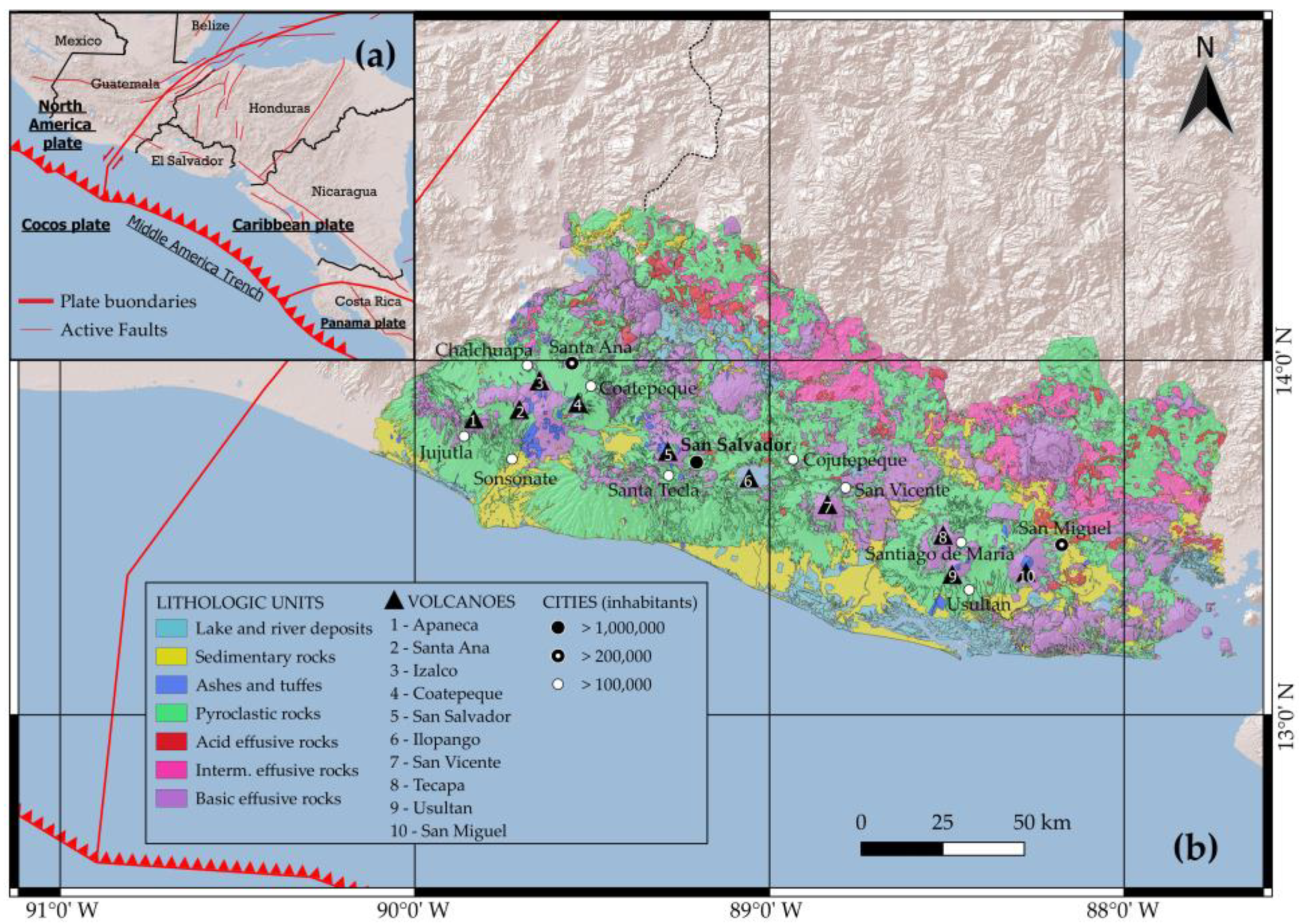
The complex geodynamic context in which the small country of El Salvador is located is characterized by the convergence of the Cocos plate and the Caribbean plate through the Middle America Trench at a rate of about 7 cm/year [51] (Figure 1a). This active tectonic environment is responsible for several active volcanoes in the country which are aligned in the WNW–ESE direction and have frequently erupted and deposited widespread and poorly consolidated tephra in many parts of the country [13]. These lithologies, in combination with acid pyroclastites and acid and basic effusive rocks, ensure that volcanic rocks represent 95% of the outcropping lithologies in the country (Figure 1b).

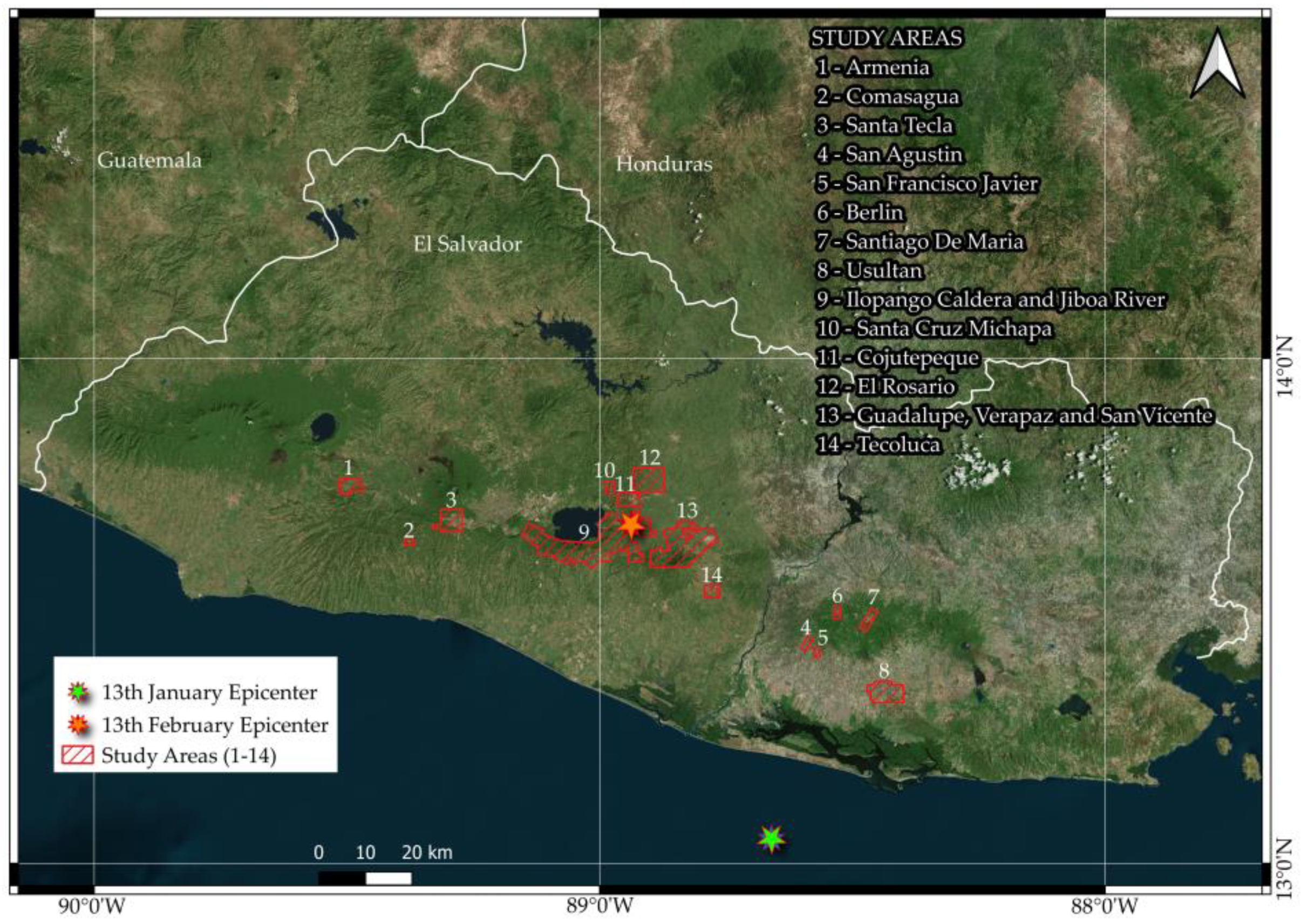
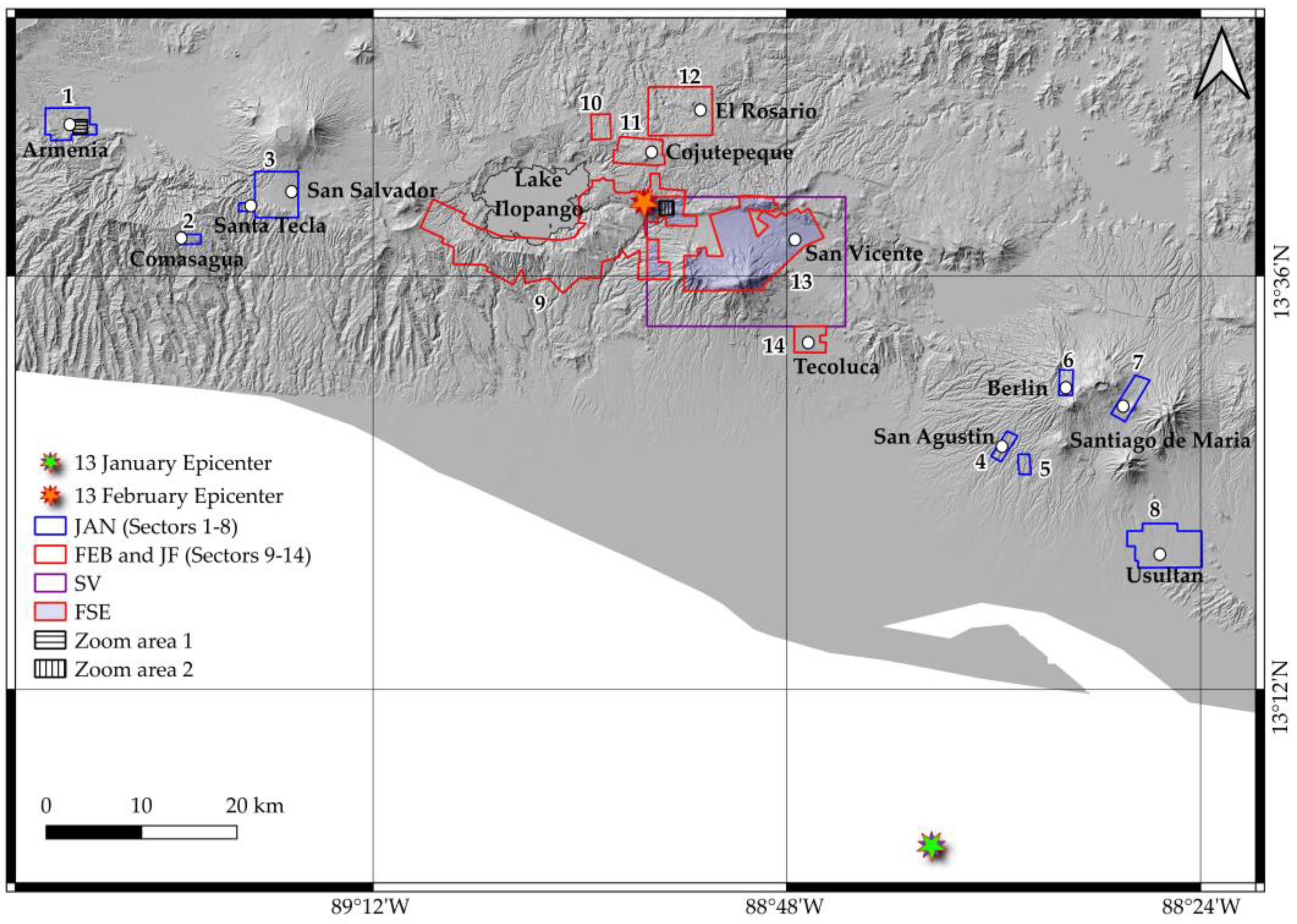
The combination of the geodynamic contexts responsible for medium and high earthquakes, steep slopes due to rugged volcanic ranges, incoherent rocks and a subtropical climate characterized by heavy storms, cause a high probability of the occurrence of earthquake- and rainfall-induced landslides in most of the country. The consequences of these gravitational phenomena are devastating for the country, which is the smallest country in Central America but has the highest population density (310 inhabitants/km²). Indeed, the fertility of the soils around the volcanoes, which are oriented WNW–ESE due to the tectonic assessment [17], has generated a situation in which a large part of the population lives in the areas of the country most susceptible to the gravitational phenomena (Figure 1b). As a confirmation of this, El Salvador has the highest ratio of destroyed houses to affected risks in Central America [52]. This work was carried out in fourteen sectors along the volcanic chain (Figure 2), which were among the areas most affected by the two intense earthquakes that occurred in the first two months of 2001.

The first eight study areas, numbered from 1 to 8, were selected because of the high number of landslides triggered by the January 2001 earthquake. Sectors 1 to 3 are in the southwestern part of the country, close to the San Salvador volcano, whereas sectors 4 to 8 are located in the southeastern portion of El Salvador. Sectors 9 to 14 are placed in the southern central part of the country and were selected because they were close to the epicenter of the February 2001 earthquake and were strongly affected by coseismic landslides.

Table 1. Extent, average and standard deviation of altitude and slope angle and the main outcropping lithology classes. GEO1: incoherent soils/rock (alluvial, marine and lacustrine deposits); GEO2: soft rocks (intermediate basic effusive rocks and subordinate pyroclastites); GEO3: hard rocks (intermediate basic effusive rocks); GEO4: medium rocks (acid effusive and acid intermediate rocks); GEO5: very soft soils (Tierra Blanca: acidic pyroclastites, subordinate volcanic epiclastites and acid effusive rocks); GEO6: soft soils (quaternary sedimentary deposits); GEO7: hard soils (acid pyroclastic rocks; volcanic epiclastites); GEO8: medium soils (volcanic epiclastites and pyroclastites; locally effusive basic–intermediate rocks).

Sector	Area [km2]	Altitude [m a.s.l.]		Slope Angle [°]		Two Main Lithology Classes
		Mean	Std. Dev.	Mean	Std. Dev.
1	15.41	577.73	64.19	15.10	11.22	GEO8 (83.92%)	GEO3 (15.39%)
2	2.31	1039.00	50.69	25.17	10.02	GEO3 (84.42%)	GEO8 (15.58%)
3	23.89	975.86	70.16	14.71	12.96	GEO8 (42.38%)	GEO5 (26.70%)
4	3.98	286.16	41.14	20.51	10.71	GEO8 (100.00%)	-
5	2.66	287.80	31.01	16.38	9.41	GEO8 (98.44%)	GEO2 (1.56%)
6	3.89	1008.35	85.91	12.11	9.23	GEO2 (72.80%)	GEO8 (27.20%)
7	8.29	862.50	70.54	11.05	8.79	GEO2 (50.97%)	GEO8 (49.03%)
8	31.42	78.34	22.40	3.29	4.28	GEO8 (95.32%)	GEO6 (1.81%)
9	155.32	618.41	122.58	24.23	12.43	GEO8 (30.17%)	GEO7 (27.98%)
10	5.32	685.48	28.97	16.46	12.00	GEO7 (56.19%)	GEO5 (41.14%)
11	13.79	781.87	74.31	16.09	10.14	GEO3 (51.69%)	GEO7 (31.39%)
12	34.80	699.61	51.11	16.30	10.01	GEO3 (10.39%)	GEO7 (73.24%)
13	87.65	833.88	365.10	17.93	13.55	GEO5 (36.26%)	GEO2 (31.78%)
14	8.84	266.62	39.17	5.12	5.55	GEO7 (90.25%)	GEO3 (8.57%)

reports the extent, average and standard deviation of the altitude and slope angle and the main outcropping lithology of all the study areas.

2.2. The 2001 Earthquakes

El Salvador has been severely affected by medium- and high-intensity earthquakes that have triggered numerous and devastating landslides. Bommer et al. [17] report that the country is experiencing earthquakes from two major seismic sources. The first source of seismicity originates from deep earthquakes in the Benioff–Wadati zones of the subducted Cocos plate beneath the Caribbean plate, which are characterized by relatively high magnitude values (often with surface wave magnitude, Ms, and moment magnitude, Mw, values of >6.0), capable of involving large areas of El Salvador. Numerous seismic phenomena with this genesis were witnessed in the last century, many of which were particularly destructive and had dramatic impacts on the country. Among these phenomena were the September 1915 event, Ms 7.8, which caused destruction in the country’s western area, and the Ms 7.3 earthquake in June 1982, which caused hundreds of earthquake-induced landslides and had 49 victims. The second source of seismicity is a zone of upper-crustal earthquakes that coincides with the array of volcanoes and is orientated WNW–ESE [17]. These intraplaque earthquakes occur at relatively lower hypocentral depths. Since the main Salvadoran cities are located just along the volcanoes’ alignment, it is not hard to determine the catastrophic consequences of the seismic events that can occur, often with more significant damage than the seismic phenomena originating in Benioff–Wadati zones. Among the most significant events of this origin in the last century are the earthquake of 8 June 1917 (Ms 6.7), which had 101 victims, the 20 December 1936 (Ms 6.1) event, which resulted in more than 200 victims, and the 10 October 1986 event (Ms 7.5), which produced more than 1500 fatalities.

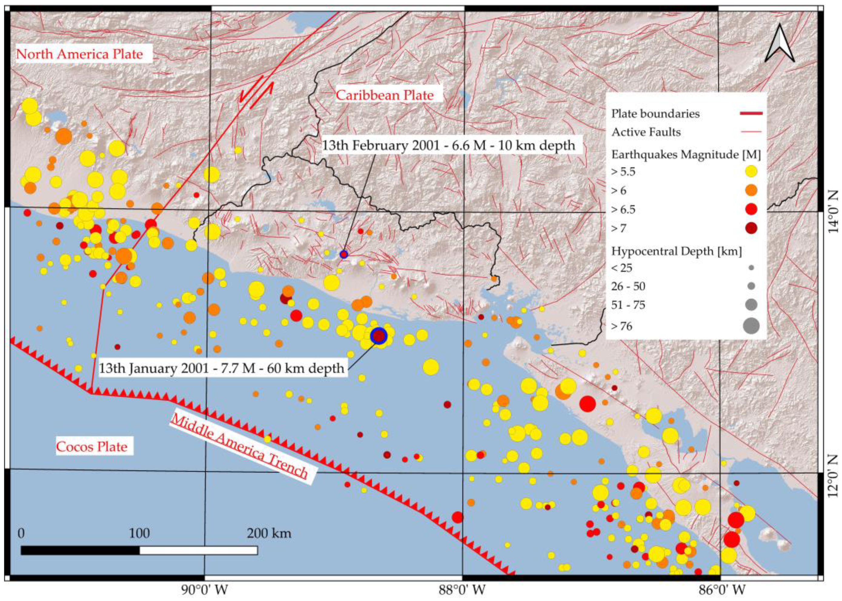
On 13 January 2001, the country was hit by a violent earthquake, originating from the first source of seismicity, at a depth of 60 km with a magnitude of 7.7 Mw (Figure 3). This event caused thousands of gravitational phenomena, injuring 5565, causing 844 fatalities and destroying over 100,000 buildings. The differences in damage and fatalities between this event and the one in 1982, which was of a similar magnitude, are related to the increase in the elements at risk. Indeed, a rapid expansion of urban areas occurred during this time span, which continued to grow mainly toward the flanks of the volcanoes, as revealed by the difference between the topographical maps of the country dating back to the year 1981 and aerial photos from 2001.

Exactly one month later, on 13 February 2001, El Salvador experienced another intense earthquake, which increased the destruction experienced by the country. This event, originating from the second source of seismicity, had a Mw of 6.6, with a hypocenter placed at a depth of 10 km. This earthquake resulted in 315 fatalities and injured 3399 people due to ground-shaking and landslides (Figure 3).

Nearly 45,000 homes were destroyed and 16,000 were seriously damaged. This earthquake affected areas comparable to those affected by the 1936 event, which was of the same genesis. Once again, the increased risk factors have led to more damage and more victims.

Most of the landslides triggered by the 2001 earthquakes were shallow debris flows; however, there were also numerous slides and debris and rock falls, according to Cruden and Varnes’ classification of landslides [53]. Moreover, both earthquakes triggered a few large and deep landslides that were highly damaging.

There are several doubts about whether these two earthquakes were related. However, some studies [17,54] reported that normal faulting subduction earthquakes in Central America tend to be followed by either large thrust events or shallow intraplate events within four years. This trend can also be observed in El Salvador, where earthquakes belonging to the second type of seismic genesis have occurred even after a month, as in the case of the earthquakes of 2001. To mention other examples of this trend, Bommer et al. [17] cited subduction earthquakes that occurred in 1915, 1932 and 1982 and were followed by intra-crustal earthquakes dated 1917, 1936 and 1986, respectively.

El Salvador is in a tropical humid climate system characterized by a dry season from November to April and a wet season from May to October in which about 75% of the annual precipitation falls. The earthquakes of 2001 occurred in the first two months of the year and thus during the dry season, as confirmed by the precipitation data recorded close to the study areas. Furthermore, the cumulative precipitation in the 12 months preceding the earthquakes of 2001 was lower than the annual average recorded at the same gauge stations in the 29 years before the earthquakes (

Table 2. Precipitation in the 12 months preceding the seismic events of 2001 and the average annual precipitation in 1971–1999 in the fourteen areas under consideration.

Sector	1	2	3	4	5	6	7	8	9	10	11	12	13	14
Rainfall [mm] March 2000–February 2001	1166	1614	1614	1571	1571	1571	1571	1571	1632	1632	1632	1632	1632	1632
Average rainfall [mm] 1971–1999	1657	1847	1847	1650	1650	1650	1650	1650	1836	1836	1836	1836	1836	1836

).

In addition, November 2000 was the last month that experienced rainfall, which was lower than the average, and unlike the averages of previous years, the following months until the earthquakes of 2001 were without rain. These data suggest that the water content did not play a decisive role in the genesis of gravitational phenomena due to the absence of or low water pore pressure in static conditions and the presence of a relatively high apparent cohesion in pyroclastic soils due to suction.

2.3. Mapping Strategy

Landslide inventories are valuable tools for investigating landscape susceptibility to these phenomena. When investigating the slope’s response to a specific triggering event, the archive must exclude the landslides that occurred before and after that event. In stochastic and empirical assessment of landslide susceptibility, the presence or absence of a gravitational phenomenon within a selected mapping unit is employed as dependent variable. Thus, the accuracy and degree of completeness of the inventory largely affect the predictive performance of the models [47,55,56,57,58].

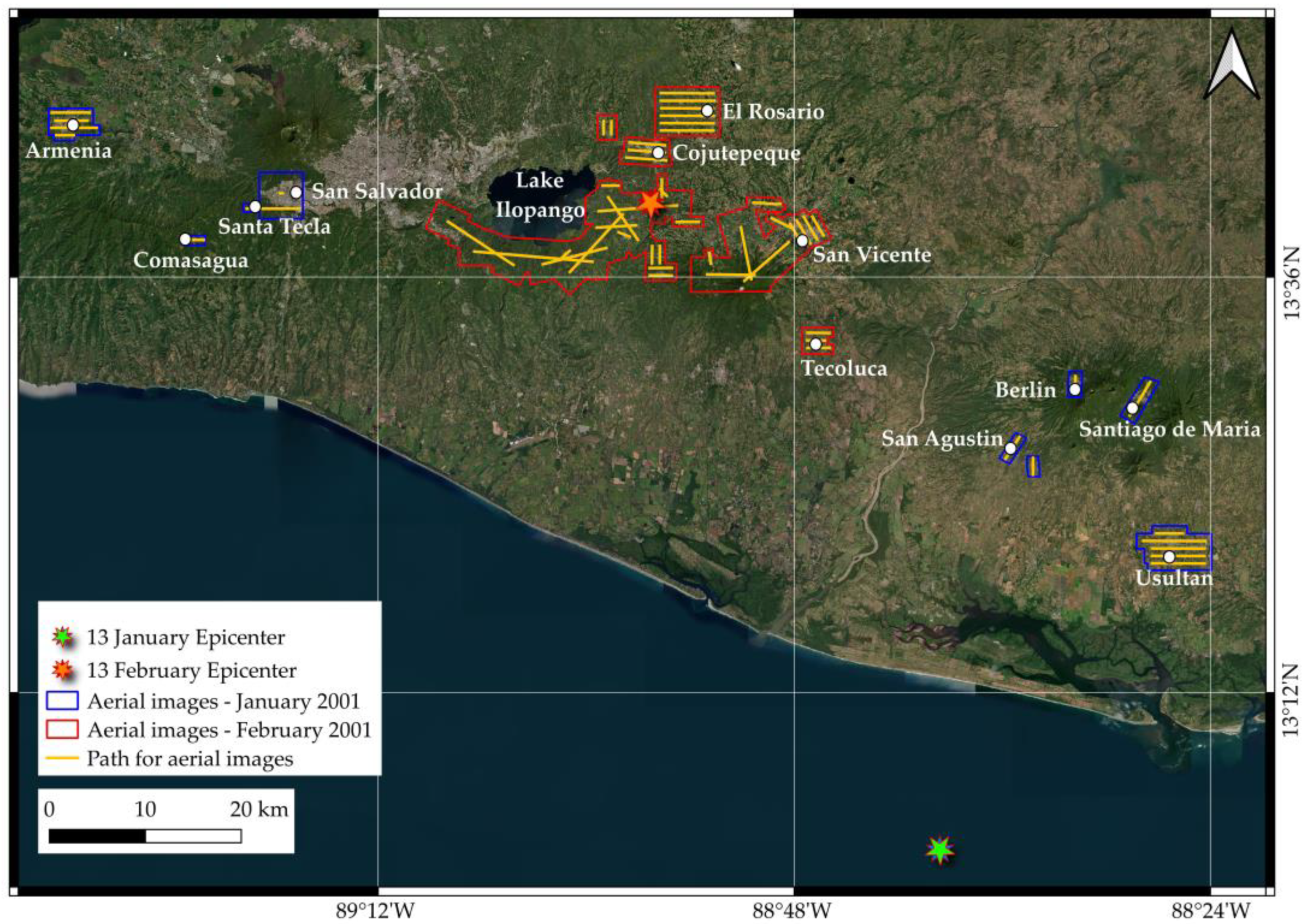
The 2001 landslide inventories available to date are incomplete, as they only include the main gravitational phenomena; therefore, the first step of this study was to prepare a complete inventory of the slope failures triggered by the two earthquake events in the study areas. To this aim, aerial photos provided by the CNR (Centro Nacional de Registros de El Salvador—Instituto Geográfico y del Catastro Nacional) were employed. Regarding the January earthquake, 136 aerial photos covering an area of 91.85 km² were analyzed, while 313 aerial photos acquired over an area of 305.72 km² were employed to identify the landslides triggered by the February earthquake (Figure 4).

Recognizing and mapping landslides in tropical areas where vegetation recovers rapidly requires aerial/satellite images taken not long after the event. The employed aerial photos were taken in the days just after the earthquakes, when the displaced materials had not yet been removed or covered by vegetation. The aerial images cover the areas of the country that were the most heavily affected by the 2001 earthquakes. These correspond to sectors of the eastern and western parts of the country in the case of the January earthquake, and to the central sector in the case of the February earthquake. To exclude slope failures triggered by a previous seismic or rainy event from the analysis, we analyzed a SPOT-4 satellite image dated 27 November 2000 (Scene ID: 4 611-323 00-11-27 16:42 2M) with 10 m spatial resolution (European Space Agency). In addition, in the areas covered by the February 2001 aerial photos, SPOT-4 satellite images from 21 January (Scene ID: 1 611-323 01-01-21 16:44 1P) were also analyzed to identify those landslides triggered by the January earthquake. It is worth noting that the aerial and satellite images allowed us to detect only landslides due to slope collapses; thus, landslide-producing fracturing and tension cracks from short coseismic slides were not included in the inventories.

In this study, the landslides were recognized, and their bodies were mapped as vector polygons. Then, the highest point of each landslide crown was identified, assuming that the environmental properties of these points, known as LIPs (landslide identification points) [23,59,60,61], reflect the pre-failure conditions that favored the initiation of the landslides.

2.4. Dependent and Independent Variables

Landslide susceptibility assessment involves dividing the study area into mapping units, which usually correspond to grid cells or slope units [29,62,63]. As grid cell partition is largely and effectively employed in landslide susceptibility mapping [8,64,65], this strategy was employed in our experiment. The study areas were resampled into 10 m pixels resulting from rescaling a 5 m cell DEM from the European Space Agency (ESA). To each of these pixels, a value for the dependent and independent variables was assigned. The cell size was selected to find a compromise between the spatial resolution and computation time needed to train and test the models [64,66], taking into account that a 10 m cell partition was successfully employed in previous studies [33,67].

In this study, the dependent variable is dichotomous, taking the value 1 when a pixel hosts one or more LIPs and the value 0 when it does not intersect a LIP or a landslide body. Independent variables were selected according to data availability and their supposed direct or indirect relationships with the spatial distribution of the slope failures that occurred in the study areas [68]. The following eleven predictors, which reflect preparatory factors, were selected: Northness (N), Eastness (E), Catchment Area (C_AR), Convergence Index (C_IND), Downslope Curvature (D_CUR), Elevation (ELE), Geology (GEO), Normalized Difference Vegetation Index (NDVI), Slope (SLO), Topographic Positioning Index (TPI), Topographic Wetness Index (TWI) and Upslope Curvature (U_CUR). N and E were obtained by calculating the cosine and sine of slope aspect, respectively. The NDVI was calculated from images dated 1 January 2001 and 2 February 2001 to analyze the areas affected by the January and February 2001 events, respectively. The terrain attributes were extracted from the DEM, which is dated 2017 and is thus more recent than the 2001 earthquake events. Therefore, to avoid training and testing the models with topographic conditions altered by the slope failures, the landslide points coincided with the highest points of each crown (i.e., LIP) and the non-landslide points were randomly selected outside the landslide areas. Additionally, two trigger (i.e., depending on the earthquake characteristics) variables were also employed as covariates, namely: Peak Ground Accelerations (PGAs) and the distance from the hypocenter (DIST). The first was obtained by rasterizing the PGA maps from both earthquakes from the USGS ShakeMap website [69], while the second by producing a distance raster from the epicenter coordinates known through the USGS website.

The absence of multicollinearity among the predictors was evaluated by calculating the Variance Inflation Factor (VIF) (e.g., [32,70]) and by applying the rule of ten ([26,71] and references therein). As all the predictors exhibited a VIF value < 10, they were used to build the landslide predictive models.

Table 3. Independent variables used to model rainfall- and earthquake-induced landslides.

Independent Variable	Application for Rainfall-Induction/Earthquake-Induction Landslide Susceptibility (Y: Yes, N: No)	Type	Reference
N Northness	Y/Y	Preparatory	Geospatial Data Abstraction Library QGis
E Eastness	Y/Y	Preparatory	Geospatial Data Abstraction Library QGis
C_AR Catchment Area	Y/Y	Preparatory	SAGA GIS
C_IND Convergence Index	Y/Y	Preparatory	SAGA GIS
D_CUR Downslope Curvature	Y/Y	Preparatory	SAGA GIS
ELE Elevation	Y/Y	Preparatory	10-m DEM resampled from a 5-m DEM from ESA
DIST Epicentral Distance	N/Y	Trigger	USGS website
GEO Geology	Y/Y	Preparatory	Geological map from Schmidt-Thomé (modified)
NDVI Normalized Difference Vegetation Index	Y/Y	Preparatory	Terra/MODIS Satellite NASA
PGA Peak Ground Acceleration	N/Y	Trigger	USGS Shakemap
SLO Slope	Y/Y	Preparatory	Geospatial Data Abstraction Library QGis
TPI Topographic Positioning Index	Y/Y	Preparatory	Geospatial Data Abstraction Library QGis
TWI Topographic Wetness Index	Y/Y	Preparatory	SAGA GIS
U_CUR Upslope Curvature	Y/Y	Preparatory	SAGA GIS

summarizes the variables employed to model the landslide spatial distribution.

2.5. Modeling Technique

The likelihood of landslide occurrence at each 10 m grid cell of the study area was calculated using multivariate adaptive regression splines (MARS; [72]) as a modeling technique. MARS is a non-parametric regression method that is useful for handling complex data and is able to model non-linear relationships between dependent and independent variables, splitting their range into an optimized number of linear branches. The extreme values of these intervals, called knots, allow an optimal linear function known as a basis function (BF). The result is a weighted sum of terms which includes a basis function or the product of two or more of them. The MARS regression function is expressed as (1):

$$y=f\left(x\right)=\alpha +{\displaystyle \sum }_{i=1}^N{\beta }_i{h}_i\left(x\right)$$

(1)

where y is the dependent variable predicted by the function f(x), α is the constant, each h_i(x) is a BF and β_i its coefficients, and N is the number of functions.

The calibration and validation of the MARS models were carried out by using the following R software packages: “raster” [73], “usdm” [74], “splitstackshape” [75], “pROC” [76], “ROCR” [77], “caret” [78], ”sperrorest” [43] and “earth” [79].

2.6. Calibration and Validation Strategy

In this study, the landslide predictive models were calibrated and validated using five datasets (Figure 5;

Table 4. Datasets used to calibrate and validate the landslide predictive models.

Dataset Code	Area	Trigger	Landslides Date
SV	San Vicente area (Mercurio et al., 2021 [49])	Rainfall	November 2009
JAN	Sectors 1 to 8	Earthquake	January 2001
FEB	Sectors 9 to 14	Earthquake	February 2001
JF	Sectors 9 to 14	Earthquake	January 2001
FSE	Intersections between FEB and SV areas	Earthquake	February 2001

), which correspond to the fourteen study sectors (JAN, FEB and JF), to the area of the San Vicente (SV) volcano landslide inventory prepared by Mercurio et al. [49] and to the intersection between the latter and sectors 9 and 13 (FSE).

These datasets are matrices in which rows correspond to the pixels of a specific area, and columns report the values of the dependent and independent variables calculated for each pixel. The dataset of rainfall-triggered landslides (i.e., SV) includes only preparatory covariates, whereas those of the coseismic landslides (i.e., JAN, FEB, JF and FSE) report the values of both preparatory and trigger variables.

The MARS predictive models were prepared using different calibration datasets or sets of predictors (

Table 5. Inventories and independent variables used in M1, M2, M3 and M4 models.

Inventory for Calibration	Model
	M1	M2	M3	M4
SV (rainfall induction)	X
JAN, JF, FEB and FSE (earthquake induction)		X	X	X
Independent variables
PSV			X
Ten preparatory variables	X			X
Two trigger variables		X	X	X
Area/Inventory for validation
JAN, JF, FEB and FSE (earthquake induction)	X	X	X	X

). The models named M1 were trained with the dataset SV, which includes rainfall-induced landslides and eleven independent variables reflecting preparatory factors. The M1 model calibrated with the dataset SV was then transferred to all fourteen study sectors of El Salvador, calculating a probability (PSV) of landslide occurrence for each pixel of these areas. The PSV values were then employed as new predictors when training the M3 model. The M2, M3 and M4 models were calibrated with the earthquake-induced landslides of January and February 2001. The variables PGA and DIST were used in the M2 model as the only covariates and in the M3 model in addition to PSV. The M4 model contains both preparatory and triggering independent variables.

The predictive ability of the M1 models was evaluated by comparing the PSV values and the presence or absence of coseismic landslides in the datasets JAN, FEB, JF and FSE.

The MARS models were calibrated and validated using three strategies. The first and second strategies consisted of the following steps. First, we randomly selected ten subsets from each dataset, which included all the event cells and the same number of non-event cells. The subsets of cells extracted from the SV dataset were used to train ten M1 models. Second, we extracted two calibration samples from the ten subsets of all the datasets, excluding SV, by randomly selecting 75% and 5% of the event cells, respectively. The remaining event cells (25% and 95%, respectively) were included in the validation samples. Both calibration and validation samples were completed by randomly selecting the same number of non-event cells. Thus, this second step produced twenty calibration and twenty validation samples from the datasets JAN, FEB, JF and FSE. The two ratios of calibration/validation samples were chosen in order to evaluate the predictive performance of the MARS models under two different scenarios: in the first scenario, the position of a large part (i.e., 75%) of the earthquake-induced landslides is known; the second scenario simulates the situation just after the earthquake occurrence, when only a very small part (i.e., 5%) of the landslides had been identified. The probability of landslide occurrence was calculated for each cell of the validation samples by averaging the score obtained from the ten MARS model runs (one for every calibration sample). This strategy was applied to increase the stability of the landslide predictions and mitigate the rare-events issue [22,32,80,81].

To further evaluate the reliability of the models, a k-fold spatial cross-validation (CV) strategy was also adopted [44,82]. According to this approach, the models are trained for k-1 combined samples at time and validated using the remaining sample. This procedure is repeated k times. Unlike the classic k-fold cross-validation approach, a sample is extracted from each of k different areas. In this study, five (k = 5) different sampling areas were identified by applying the k-means clustering algorithm. Similarly, to the first and second calibration and validation strategy, the spatial CV was repeated ten times in order to assess the robustness of the models.

For all the validation samples, a receiver operating characteristics (ROC) curve [42,48,71,83] was prepared using the average MARS score to predict the value of the dependent variable at each pixel (0: LIP absence; 1: LIP presence). The ROC curve plots sensitivity (true positive rate) against 1—specificity (false positive rate). Then, the area under the ROC (AUC) curves were calculated, thus obtaining ten AUC values for the prediction of the datasets JAN, FEB, JF and FSE for each of the models M1 to M4 and validation scenarios. This procedure led to a total of 480 AUC values. An AUC value close to 0.5 reveals a random prediction, whereas a value of 1.0 reflects a perfect ability to discriminate between event and non-event pixels. AUC values larger than 0.7, 0.8 and 0.9 were considered as acceptable, excellent and outstanding, respectively [84]. The Wilcoxon signed-rank test was employed to identify significant differences between the predictive skill performance of the models by setting the level of significance at 0.01.

2.7. Landslide Susceptibility Maps

The models M1 to M4 were used to generate a landslide susceptibility map for each of the four datasets. To this aim, we employed the MARS models calibrated with the samples including 75% of the LIPs. For each pixel of the datasets JAN, FEB, JF and FSE, a probability (P) of landslide occurrence was calculated for the models M1, M2, M3 and M4 by averaging the score of their ten repetitions. Since the models were trained on samples including the same number of LIP and non-LIP locations, P should be interpreted as the spatial relative probability of landslide occurrence.

3. Results

3.1. The 2001 Earthquake-Induced Landslide Inventories

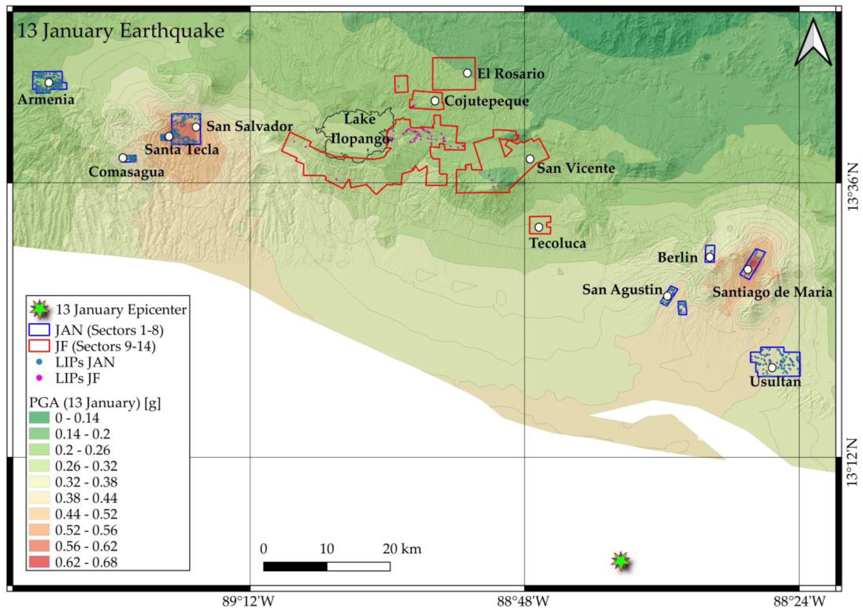
The landslide inventory of the dataset JAN was obtained by analyzing eight sets of aerial photos taken a few days after the earthquake of 13 January 2001. These images cover eight inhabited sectors, extending for 91.85 km² (Figure 6), which experienced the most significant damage due to the seismic shaking and the consequent landslides. These were mainly rotational slides, debris/earth flows and earth/rock falls.

The inventory consists of 997 LIPs, each hosted by a 10 m pixel. The percentage of event cells (i.e., cells hosting at least one LIP) compared to the total number of pixels (1,260,811) of the study area is equal to 0.08%, while there are 9556 cells intersecting the landslide polygons, corresponding to 0.76% of the total pixels. The JF inventory includes the LIPs and landslides caused by the January earthquake in the areas covered by the aerial images taken after the February event (sectors 9 to 14, counted from west to east, are Ilopango south and Rio Jiboa, S. Cruz Michapa, Cojutepeque, El Rosario, San Vicente and Tecoluca, respectively; red polygons of Figure 6). These landslides were identified by analyzing images from the SPOT-4 satellite dated 21 January 2001. In these sectors, with relatively low January PGA values, 123 LIPs were mapped, each placed in one 10 m cell and accounting for 0.002% of the total number of cells of the area under examination. When landslide bodies are considered, unstable pixels cover 0.2% of the area.

When the JAN and JF inventories are merged, the percentages of LIPs and landslide pixels in relation to the total area (sectors 1 to 14) are significantly reduced (0.017 and 0.30, respectively) due to the low PGA values within sectors 9 to 14. However, the landslides triggered in these sectors, despite being about one tenth of the number of the JAN landslides, cover a significantly higher number of pixels (

Table 6. Amounts and characteristics of the landslides triggered by the January earthquake in sectors 1 to 14.

Sector	Area of the Sector (km2)	N° of LIPs	% of Event Cells	N° of Landslides Extending <100 m2; (%)	N° of Landslides Extending 100–1000 m2; (%)	N° of Landslides Extending 1000–10,000 m2; (%)	N° of Landslides Extending >10,000 m2; (%)	Landslides’ Average Extent in m2	% of Landslide Cells
1	15.41	245	0.10	84 (34.29)	143 (58.37)	18 (7.35)	0 (0)	297.69	1.24
2	2.31	128	0.52	67 (52.34)	57 (44.53)	4 (3.13)	0 (0)	190.91	3.16
3	23.89	296	0.10	107 (36.15)	159 (53.72)	28 (9.46)	2 (0.68)	870.79	1.45
4	3.98	67	0.07	38 (56.72)	29 (43.28)	0 (0)	0 (0)	145.82	0.39
5	2.66	43	0.15	27 (62.79)	14 (32.56)	2 (4.65)	0 (0)	151.94	0.74
6	3.89	8	0.02	1 (12.50)	6 (75.00)	1 (12.50)	0 (0)	328.59	0.19
7	8.29	17	0.01	1 (5.88)	16 (94.12)	0 (0)	0 (0)	267.09	0.06
8	31.42	193	0.05	88 (45.60)	103 (56.37)	2 (1.04)	0 (0)	116.19	0.31
JAN (1–8)	91.85	997	0.08	413 (41.42)	527 (52.86)	55 (5.52)	2 (0.20)	407.13	0.76
9	155.32	93	0.0025	0 (0)	19 (20.43)	55 (59.14)	19 (20.43)	8744.50	0.27
10	5.32	1	0.0018	0 (0)	0 (0)	0 (0)	1 (100)	19,571.39	0.44
11	13.79	23	0.0136	0 (0)	8 (34.78)	15 (65.22)	0 (0)	2079.28	0.35
12	34.80	0	0	0 (0)	0 (0)	0 (0)	0 (0)	0	0
13	87.65	6	0.004	0 (0)	1 (16.67)	3 (50.00)	2 (33.33)	10,263.87	0.05
14	8.84	0	0	0 (0)	0 (0)	0 (0)	0 (0)	0	0
JF (9–14)	305.72	123	0.002	0 (0)	28 (22.77)	73 (59.34)	22 (17.89)	7660.25	0.20
JAN + JF (1–14)	397.57	1120	0.017	413 (36.88)	555 (49.56)	128 (11.42)	24 (2.14)	3585.67	0.30

). This can be explained considering that the steepest slopes are characterized by thick deposits of poorly consolidated late Pleistocene and Holocene Tierra Blanca rhyolitic tephras that erupted from Ilopango caldera, an area particularly susceptible to the initiation of gravitational phenomena [47,61]. In fact, in that region, the January earthquake resulted in a low number of debris flows and rotational slides; however, they had a large extent. This is also demonstrated by the number of gravitational phenomena that were larger than 10,000 m²: two and twenty-two in the JAN and the JF datasets, respectively. However, two gravitational phenomena, which both occurred in sector 3 (Las Colinas neighborhood of Santa Tecla, west of the capital San Salvador), caused the worst damage and the largest number of victims. One of these was a complex landslide (rotational slide and earth flows) that covered an area of about 200,000 m³ in which approximately 585 people lost their life. This landslide, which sadly become famous for the devastation it generated, was about 800 m long and 150 m wide, with a 50 m high escarpment activated on the north side of El Balsamo Ridge, which is composed of the andesitic cinders and some interbedded tephra of the El Balsamo Formation [17]. The second event, located approximately 2.5 km from the first landslide, was a debris flow about 1500 m long which also began from the north side of El Balsamo Ridge and reached and destroyed a sector of the Carrera Panamericana, the most crucial road in the country which connects the capital with the western part of El Salvador. The highway interruption hindered the arrival of aid, creating enormous damage to the population. However, the absence of small landslides in sectors 9 to 14 compared to that of sectors 1 to 8 (41.42%) could also be related to the different resolution of the images used for mapping, as phenomena with an extension of less than 100 m² are hardly detectable in a satellite analysis with a 10 m resolution.

The seismic phenomenon of 13 February triggered thousands of landslides in the country’s central sector. Many landslides occurred where slopes were covered by thick and slightly consolidated deposits of the rhyolitic tephras of the Tierra Blanca Formation, which originated from eruptions from the Ilopango Caldera.

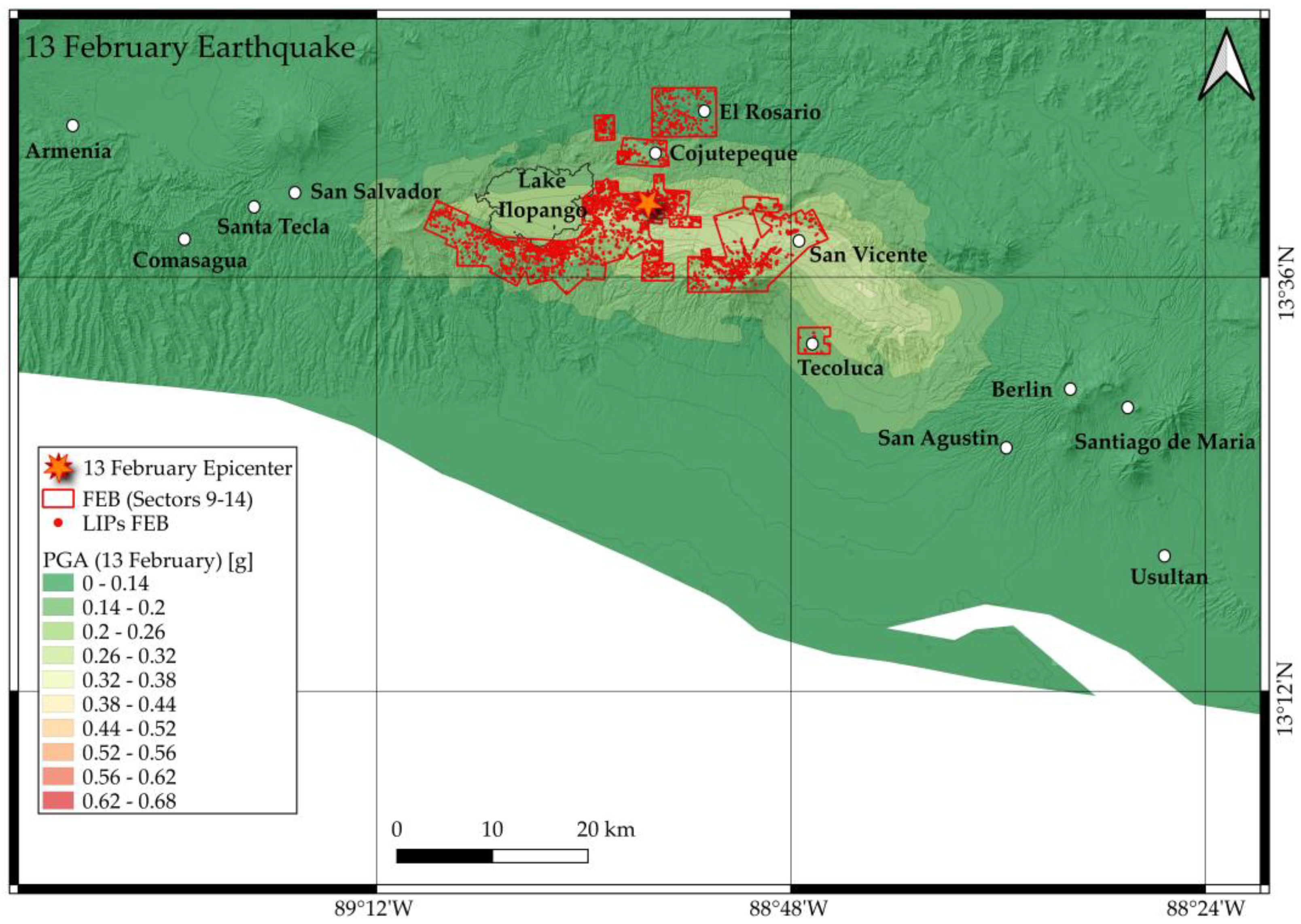
Landslide mapping was carried out using aerial photos taken a few days after the event in areas that experienced a very high PGA and suffered the most significant damage (sectors 9 to 14, Figure 7). The landslides that were also included in the JF inventory were discarded except for those that have been reactivated.

The FEB inventory includes 5371 LIPs intersecting 5344 pixels. The percentage of event cells of the FEB dataset is 0.09%. The extent of the landslide bodies is 123,488 pixels, which accounts for 2.12% of the study area. This seismic event triggered landslides similar to those of the JAN dataset, but their frequency and size were higher (

Table 7. Amounts and characteristics of the gravitational phenomena of landslides belonging to sectors 9 to 14, related to the February earthquake.

Sector	Area of the Sector (km2)	N° of LIPs	% of Event Cells	N° of Landslides Extending <100 m2; (%)	N° of Landslides Extending 100–1000 m2; (%)	N° of Landslides Extending 1000–10,000 m2; (%)	N° of Landslides Extending >10,000 m2; (%)	Landslides’ Average Extent in m2	% of Landslide Cells
9	155.32	3650	0.10	427 (11.70)	2145 (58.77)	955 (26.16)	123 (3.37)	1694.63	2.47
10	5.32	186	0.33	32 (17.20)	119 (63.98)	34 (18.28)	1 (0.54)	789.50	4.68
11	13.79	279	0.16	91 (32.62)	151 (54.12)	37 (13.26)	0 (0)	554.75	1.58
12	34.80	209	0.06	6 (2.87)	144 (68.90)	57 (27.27)	2 (0.96)	1093.83	1.16
13	87.65	1029	0.07	172 (16.72)	563 (54.71)	267 (25.95)	27 (2.62)	1500.60	1.56
14	8.84	18	0.02	8 (44.44)	10 (55.56)	0 (0)	0 (0)	126.75	0.08
FEB (9–14)	305.72	5371	0.092	736 (13.70)	3132 (58.31)	1350 (25.13)	153 (2.85)	1538.26	2.12

).

Among the many large-scale phenomena, large rotational flows of debris were mapped in the area close to the epicenter, corresponding to areas near the Jiboa River, which fortunately have low population densities. As a matter of fact, thousands of gravitational phenomena have been detected in the Tierra Blanca Formation (GEO5), some of which caused the damming of the river for hundreds of meters, causing the formation of an artificial lake that could have caused a high hydrogeological risk downstream.

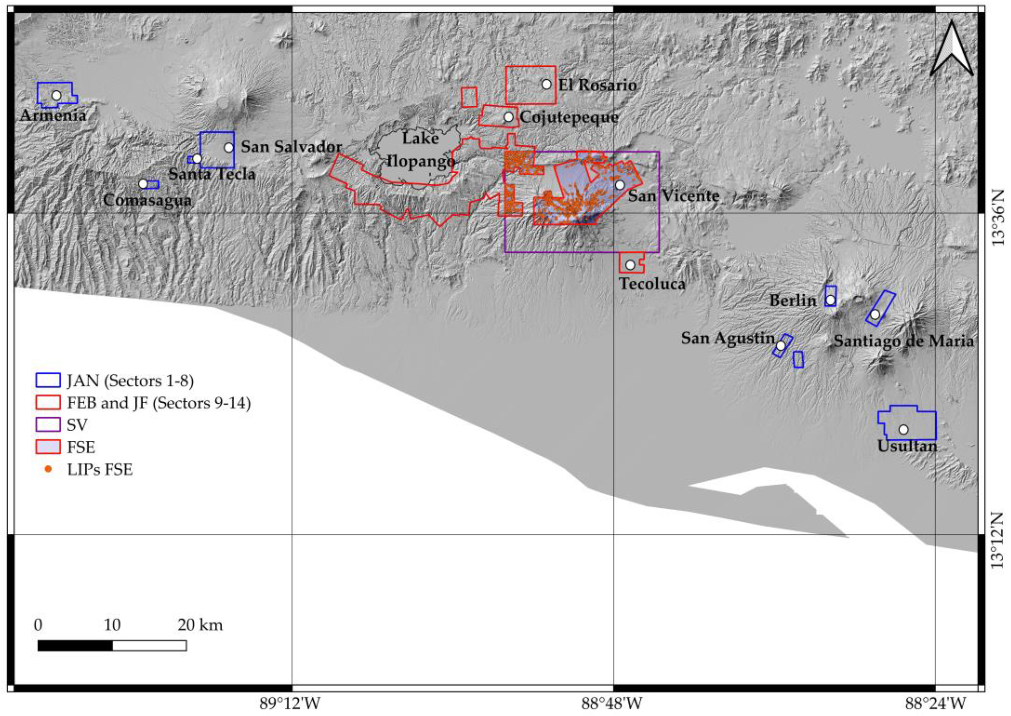
The FSE inventory was generated by overlapping the areas of the datasets FEB and SV. The intersection extended for 107 km² and included the entirety of sector 13 and 12.5% of sector 9 in the FEB study areas (Figure 8). The FSE dataset contains 1587 LIPs pertaining to the landslides triggered by the February earthquake, which were mainly earth/debris flows.

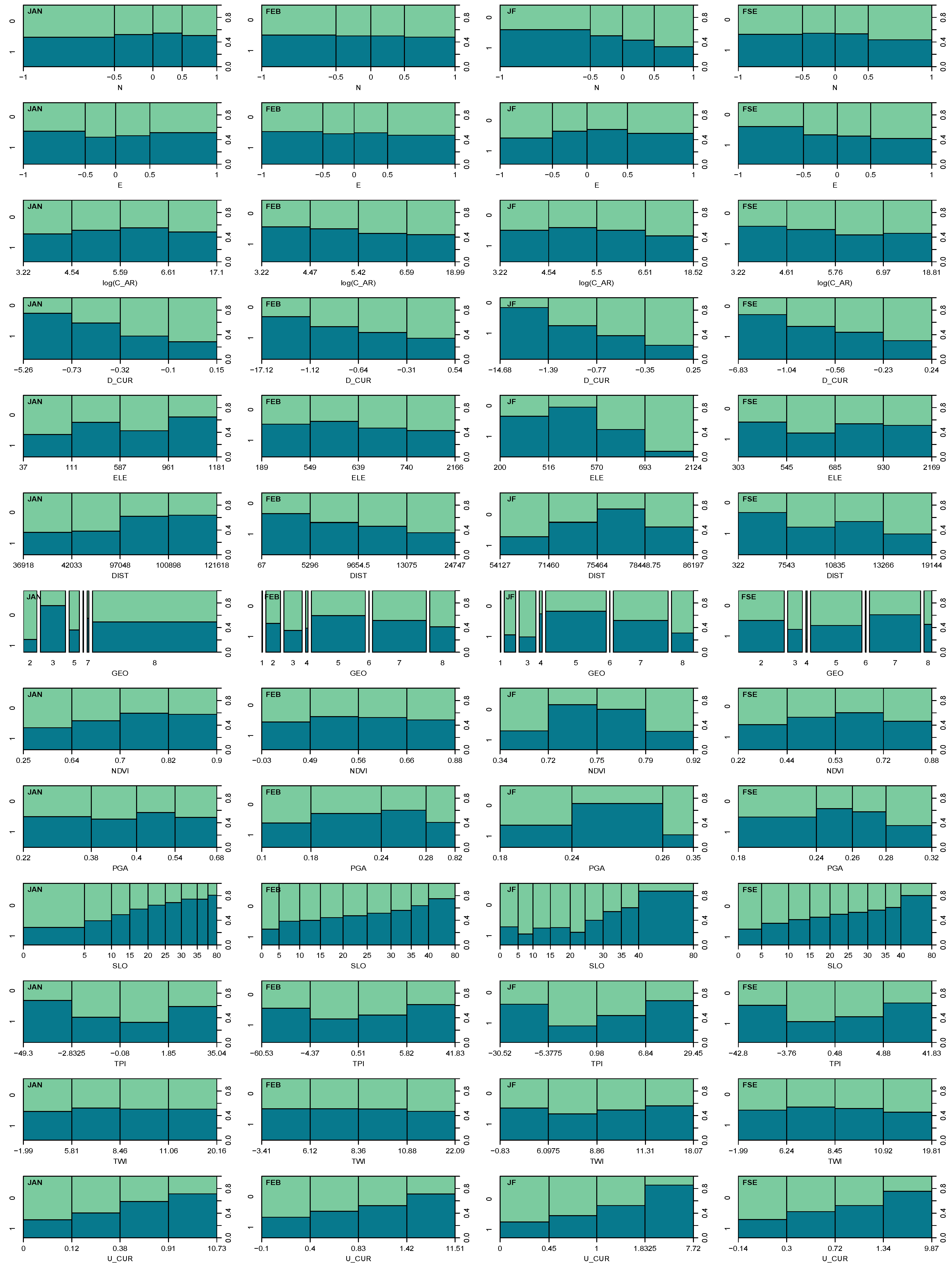
The conditional density plots of Figure 9 reveal empirical relationships between landslide inventories and independent variables. These plots show the relative frequency of non-LIP (0) and LIP (1) pixels within the predictor classes. A higher frequency of LIPs occurs in steeper slopes and where the upslope and downslope curvatures are convex and concave, respectively. The N and E plots show that landslide density was higher on the north- and east-facing slopes of the datasets JF and FSE, respectively. Landslides are very rare at high-elevation JF positions, while they are more numerous where the elevation is high in the JAN dataset. As expected, the density of February LIPs decreases with the distance from the earthquake epicenter; surprisingly, the opposite occurs for the LIPs triggered by the January seismic event. A relatively high landslide frequency is observed in hard rocks (JAN), very soft soils (FEB and JF) and hard soils (FSE), as well as in upper (positive TPI) and lower (negative TPI) slopes. The density of LIPs is slightly higher than the average in intermediate PGA classes of the datasets FEB, JF and FSE.

3.2. The Ida/96E 2009 Inventory

The SV inventory [49] covers an area of 287 km² around the flanks of the San Vicente Volcano and includes the LIPs of 5609 landslides triggered between 7 and 8 November 2009 [85] by an extreme rainfall event. This event was caused by the combined action of Hurricane Ida and the low-pressure system 96E, which produced 350 mm in 24 h in an area of about 400 km² located between Ilopango Lake and the San Vicente Volcano (Figure 8). The rainfall triggered numerous and large flows that caused fatalities and massive damage, with an economic loss of approximately a quarter of USD one billion [86].

3.3. Predictive Performance of the MARS Models

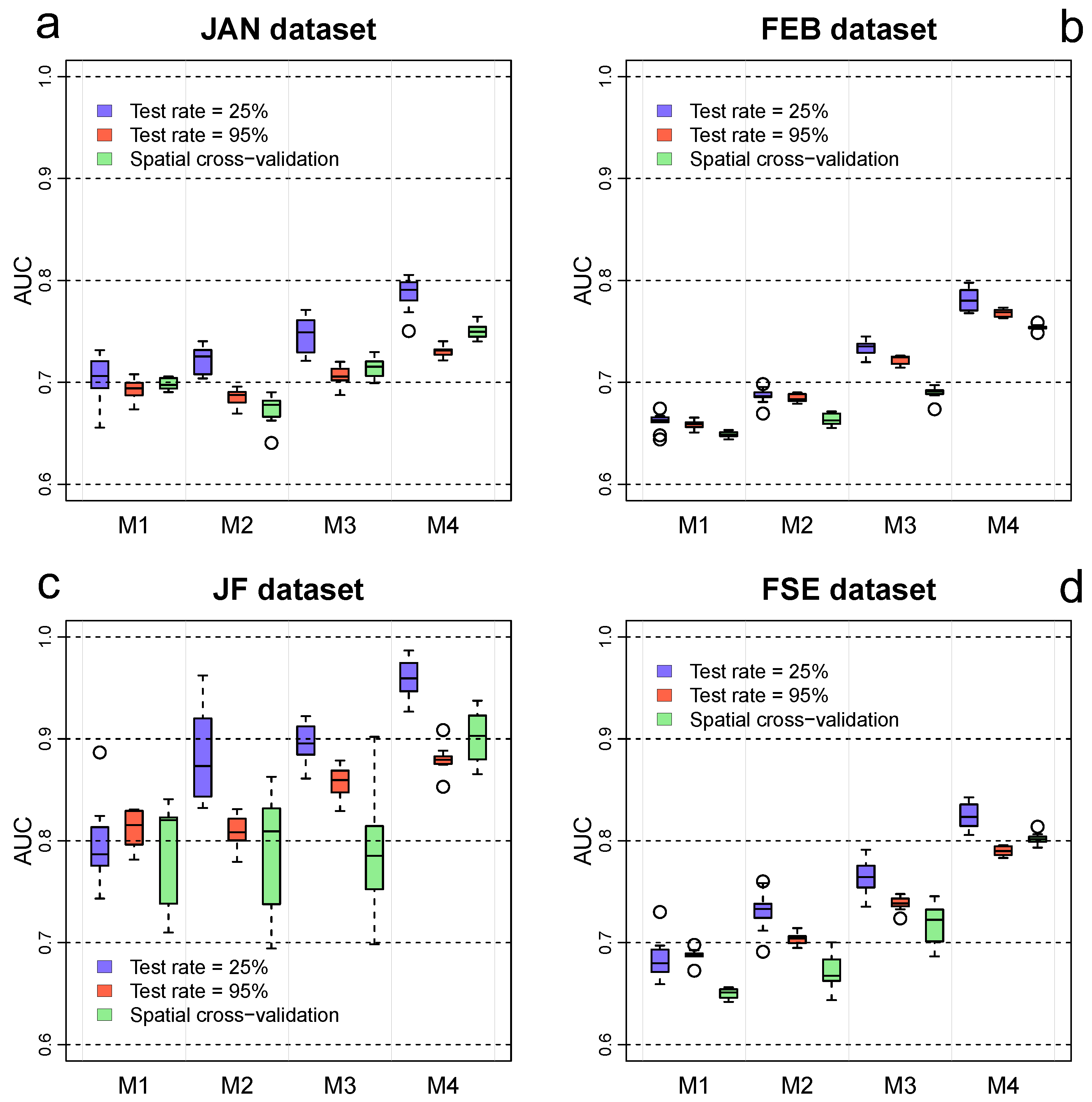
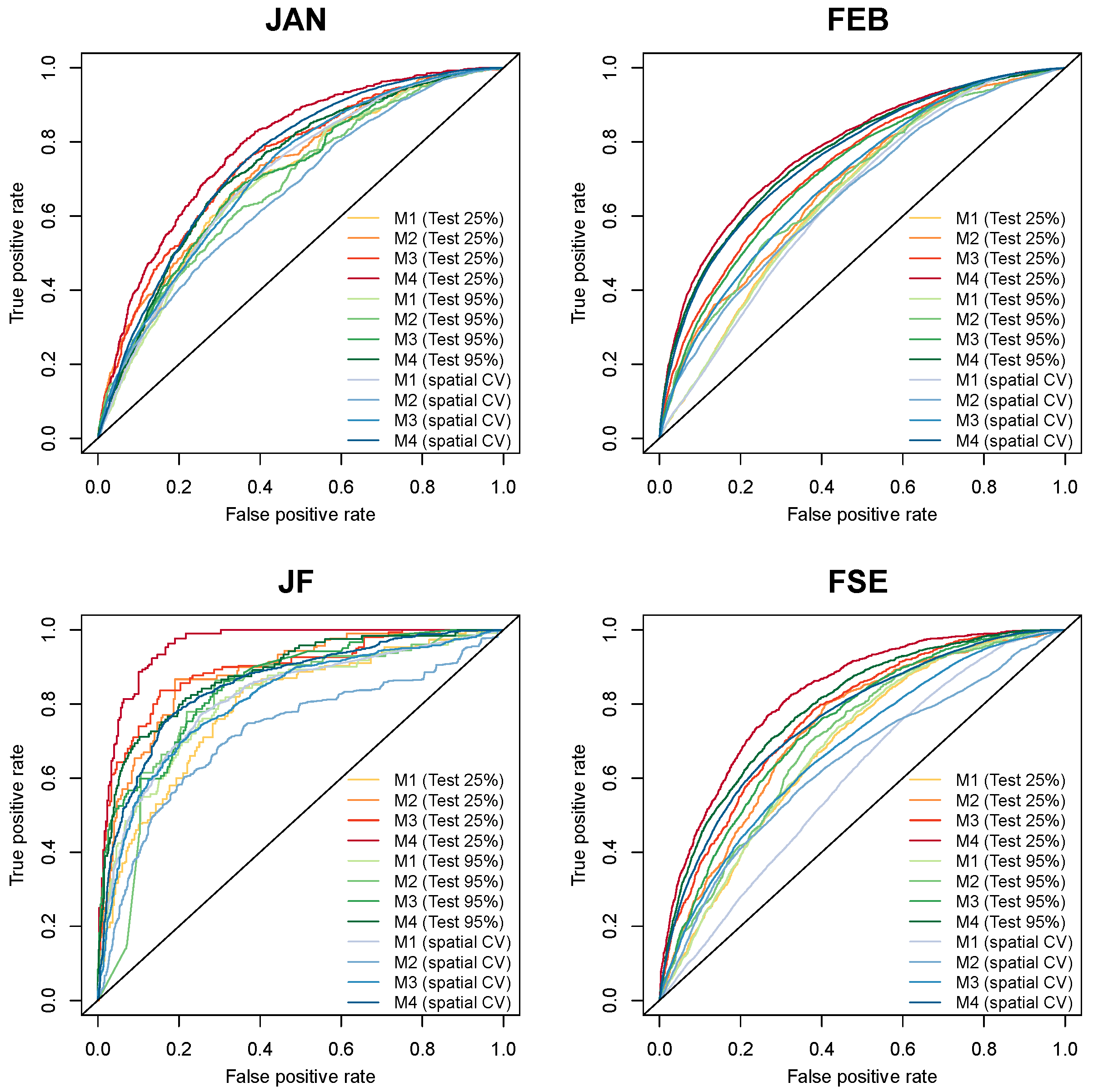
The inventories and variables used for calibrating and validating the M1, M2, M3 and M4 models are shown on Table 5. The predictive skill of the models, measured on the validation samples of the datasets JAN, FEB, JF and FSE, are revealed by the boxplots in Figure 10. These reflect, for each model and dataset, the variability and skewness of the ten AUC values calculated by applying the calibration and validation strategies described in Section 2.6. The skewness displays, for each group of ten AUCs, their first quartile (Q1), median and third quartiles (Q3), the minimum and maximum values within 1.5 times the interquartile range (IQR) above Q3 and below Q1 and eventually outliers outside 1.5 of the IQR. Moreover,

Table 8. AUC mean and standard deviation (SD) calculated for the four models and datasets, with the three validation scenarios (Scenario 1: test rate 25%; Scenario 2: test rate: 95%; Scenario 3: 5-fold spatial CV).

Scenario 1	AUC_JAN mean	AUC_JAN SD	AUC_FEB mean	AUC_FEB SD	AUC_JF mean	AUC_JF SD	AUC_FSE mean	AUC_FSE SD
M1_75	0.7	0.026	0.661	0.009	0.795	0.041	0.685	0.02
M2_75	0.723	0.013	0.687	0.008	0.88	0.042	0.731	0.02
M3_75	0.747	0.017	0.734	0.007	0.896	0.018	0.765	0.016
M4_75	0.787	0.017	0.781	0.01	0.958	0.021	0.824	0.012
Scenario 2	AUC_JAN mean	AUC_JAN SD	AUC_FEB mean	AUC_FEB SD	AUC_JF mean	AUC_JF_ SD	AUC_FSE mean	AUC_FSE SD
M1_05	0.693	0.01	0.658	0.004	0.812	0.018	0.688	0.006
M2_05	0.685	0.008	0.684	0.004	0.809	0.015	0.704	0.006
M3_05	0.706	0.009	0.722	0.004	0.857	0.016	0.739	0.007
M4_05	0.731	0.006	0.768	0.003	0.88	0.014	0.79	0.005
Scenario 3	AUC_JAN mean	AUC_JANS D	AUC_FEB mean	AUC_FEB SD	AUC_JF mean	AUC_JF_ SD	AUC_FSE mean	AUC_FSE SD
JAN_M1	0.699	0.006	0.649	0.003	0.794	0.052	0.65	0.005
JAN_M2	0.673	0.014	0.664	0.006	0.787	0.06	0.671	0.017
JAN_M3	0.714	0.01	0.69	0.006	0.792	0.068	0.718	0.019
JAN_M4	0.75	0.008	0.754	0.003	0.901	0.025	0.802	0.006

shows the average and standard deviation values of the AUC groups. Furthermore, the average ROC curves calculated for each group of ten model runs are shown in Figure 11.

The M1 models, calibrated with all rainfall-induced landslides that occurred near the San Vicente volcano and then transferred to the study areas, exhibit average AUC values ranging from 0.65 to 0.81. Overall, the accuracy of these models is poorer than that of the other models, except for what was observed in the datasets JAN and JF, where the M1 models perform similarly to the M2 models or even better when validation is carried out with 95% of the landslides or by applying the spatial CV. The average performance of the M1 models is not acceptable for the datasets FEB and FSE, whereas it is almost acceptable in the dataset JAN [84]. The M1 models show the best performance in the dataset JF, achieving a mean AUC in the range of 0.79–0.81.

The M2 models, which include as predictors the variables PGA and DIST, achieved mean AUC values in the range of 0.66–0.88. Their performance is better than the performance exhibited by the M1 models except for the dataset JAN when the validation scenarios 2 (test rate = 95%) and 3 (spatial CV) are applied. In these cases, as well as in the datasets FEB and FSE (with spatial CV), the predictive skills of the M2 models are not acceptable. On the other hand, their ability to discriminate between stable and unstable cells ranges from acceptable to excellent for the datasets FSE (with Scenarios 1 and 2) and JF.

The validation of the M3 models revealed mean AUC values in the range of 0.69–0.90, significantly higher than those achieved by the M1 and M2 models in all datasets except when applying spatial CV to the JF dataset. The average AUC achieved by the M3 models, which were fitted using the covariates PGA, DIST and PSV, ranges from acceptable to excellent, with lower values revealed by the spatial CV in the datasets FEB, JF and FSE.

The M4 models were trained with all independent variables available, excluding PSV. The validation results reveal a further improvement in the predictive ability of the M4 models compared to the predictive ability exhibited by the other models. The average AUC values, which are in the range of 0.73–0.96, exceed the acceptability threshold in the datasets JAN, FEB and FSE, achieving excellent to outstanding levels when the models are applied to the JF datasets.

The best predictive ability of the four tested models is observed in the dataset JF (mean AUC: 0.79–0.96), which contains the landslides triggered in sectors 9 to 14 by the January earthquake. Conversely, the models exhibited some inaccuracy in discriminating between stable and unstable cells of the JAN and FEB datasets, showing mean AUC values in the ranges of 0.67–0.79 and 0.65–0.78, respectively.

Overall, when the learning samples include 75% of the observed landslides, models M2 to M4 exhibit a significantly better accuracy (mean AUC: 0.69–0.96) than the accuracy achieved when they are calibrated using only 5% of the landslides (mean AUC: 0.68–0.88) or when applying the 5-fold spatial CV (mean AUC: 0.66–0.90). However, except for the dataset JF, the differences in mean AUC values are small and insignificant when the M2 models are fitted with 5% of the FEB landslides. Moreover, regarding the M1 models, there is no significant difference in accuracy when validation is carried out with 25% and 95% of the landslides. As expected, larger differences in AUCs are observed when comparing validation Scenarios 1 (test rate = 25%) and 3 (spatial CV), since the latter involves the transfer of the models between different areas.

Validation samples containing 95% of the landslides reveal a more stable predictive skill (SD: 0.003–0.018) than the predictive skill obtained when validating the models with the 25% of the event cells (SD: 0.007–0.042). The performance of the models is also stable when the spatial CV is carried out in JAN, FEB and FSE (SD: 0.003–0.019), but the AUC values are rather dispersed in JF (SD: 0.025–0.068), where Scenarios 1 (SD: 0.018–0.042) and 2 (SD: 0.014–0.018) also exhibit variability in their performances.

The ROC curves of Figure 11 confirm that predictive skill increases from the models M1 to M4. Since the FEB dataset contains the largest number of LIPs (5371), the ROC curves prepared for this dataset are smoother. Conversely, those calculated for JF are scattered, as they are derived from samples including a few landslides (123).

3.4. Comparision of the Landslide Susceptibility Maps

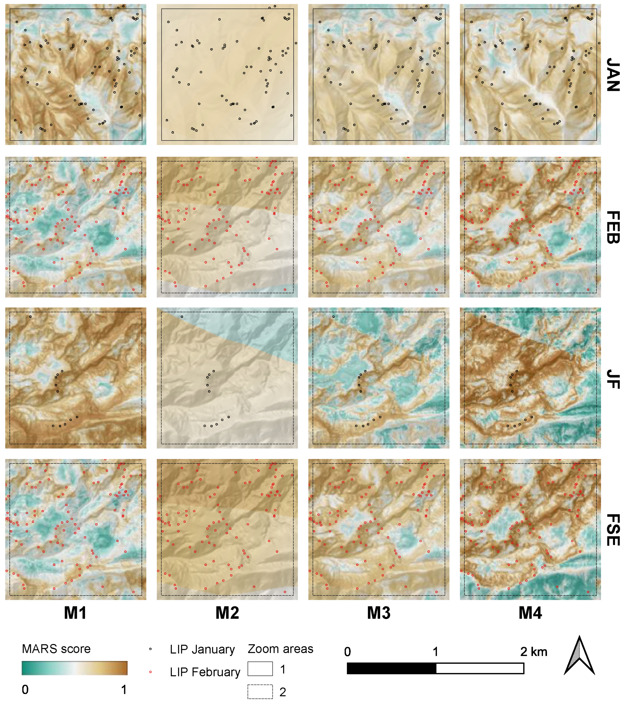
Figure 12 shows an example of the landslide susceptibility maps generated by models M1, M2, M3 and M4 for two zoom areas (Figure 5).

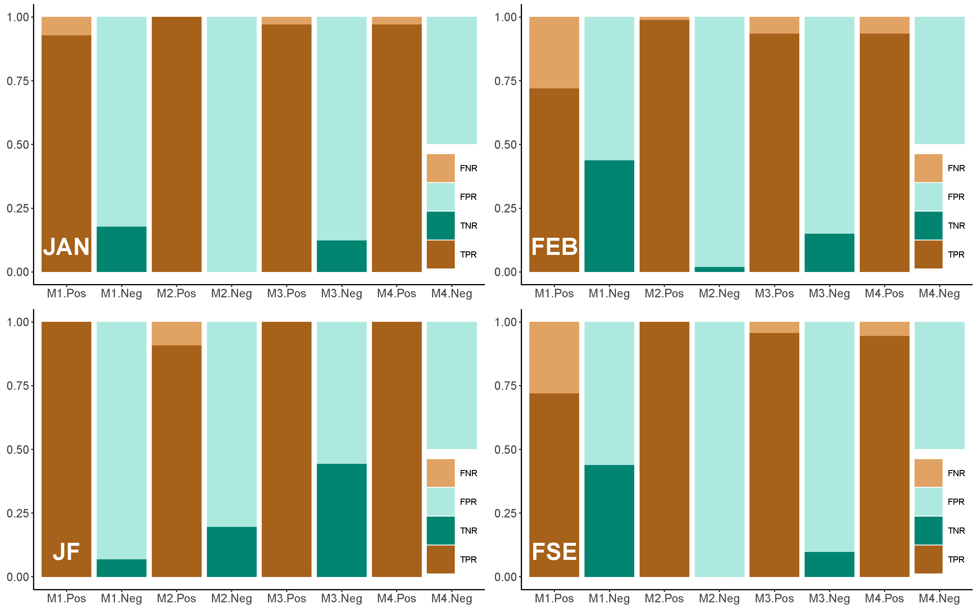
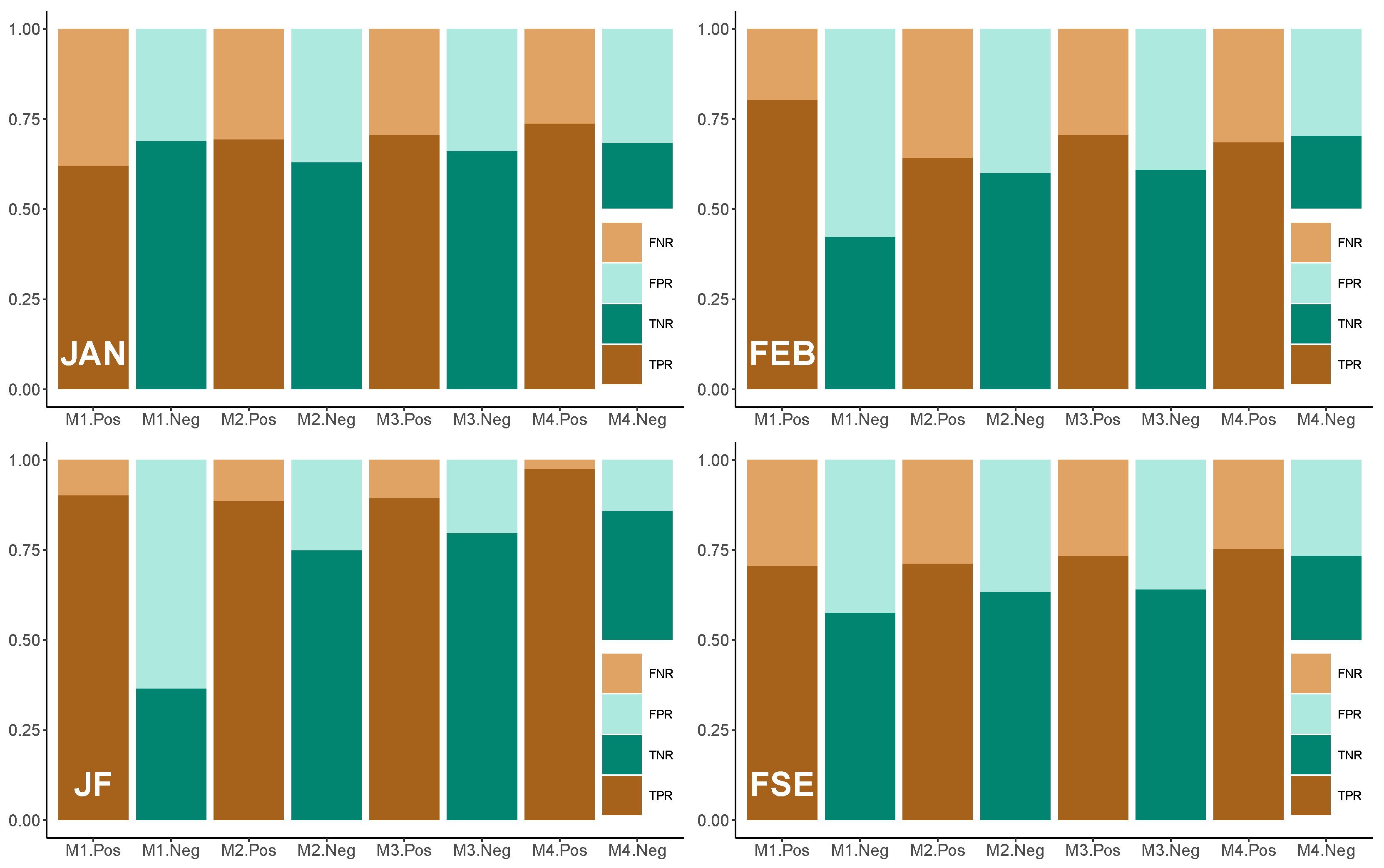
As they are landslide-prone areas, MARS score values tend to be high. Overall, maps generated by the M2 models show abrupt changes related to the pattern of PGA values, while the other maps are smoother except for the M3 and M4 maps of the dataset JF. Figure 13 and Figure 14 reveal the values of the true positive rate (TPR), true negative rate (TNR), false positive rate (FPR) and false negative rate (FNR) calculated for the zoom areas of Figure 12 and for the entire landslide susceptibility maps, respectively. These metrics were calculated by setting a probability cut-off value of 0.5. In the zoom areas, the maps exhibit a very high rate of true positive but also a very high FPR (Figure 13). This is particularly evident for the M2 and M3 models. On the other hand, the entire susceptibility maps show a better discrimination ability, with markedly lower values of FPR, even if a decrease in true positives is also observed (Figure 14). These histograms confirm that the best ability to discriminate landslide pixels is achieved for the dataset JF by the models M2 (TPR: 0.886; TNR: 0.750), M3 (TPR: 0.894; TNR: 0.797) and M4 (TPR: 0.976; TNR: 0.856).

4. Discussion

In January and February of 2001, El Salvador was hit by two intense seismic phenomena of different natures which produced thousands of gravitational phenomena. Both 2001 earthquakes triggered similar landslides, but their distribution varied because of different earthquake source parameters, such as magnitude, epicentral distance and hypocentral depth. Indeed, earthquakes with large hypocentral depths tend to produce a relatively low number of gravitational phenomena spread over large areas. In contrast, phenomena that occur at a relatively low hypocentral depth usually produce many landslides concentrated in areas close to the epicenter [10]. The seismic event of January, with a hypocentral depth of 60 km, triggered 1200 gravitational phenomena across 398 km², whereas 5371 landslides, spread over 305 km², were induced by the February event, which had a hypocentral depth of 10 km. The difference in hypocentral depth caused different spatial distributions of the PGA and MMI (modified Mercalli intensity). In fact, their values decreased from the hypocenter to a greater distance in the January event compared to the February event. The slow decay of PGA values, which is observed for earthquakes with a deep and offshore genesis, triggers gravitational phenomena over larger areas than earthquakes with the most superficial genesis. Conversely, the latter are characterized by a higher concentration of slope failures around the hypocenter.

In this work, four different MARS models (M1 to M4) were produced using different predictor sets and landslide inventories, the latter containing the slope failures triggered by the Ida/96E event of November 2009 (M1) and those induced by the earthquakes of January and February 2001 (M2 to M4). Two different calibration and validation scenarios were employed. In the first scenario, three quarters of the observed landslides were used for calibrating the models M2 to M4, whereas the remaining quarter was included in the validation samples. This scenario is frequently used to produce and validate landslide susceptibility models [65,80,87,88]. In the second scenario, the learning samples contained only 5% of the earthquake-induced landslides, using the remaining 95% of the LIPs for validation. Additionally, to further investigate the predictive skill of the models, a third validation approach based on a 5-fold spatial cross-validation (CV) was applied.

The AUC values calculated for each model, dataset, and validation scenario, which are summarized by Table 8 and the boxplots of Figure 10, reveal that the MARS algorithm provides reliable predictions of the spatial distribution of earthquake-induced landslides. Indeed, 73% of the 320 AUC values AUC that were computed by applying the two test rates (25 and 95%) exceed the threshold of acceptability (AUC > 0.7), and a quarter of them even reveal the excellent predictive skill of the models (AUC > 0.8). Regarding the spatial CV, these percentages decrease to 50% and 21%, respectively. This is related to the data-driven nature of the adopted approach, which may generate a very good ability to predict unknown events if calibration and validation samples are extracted from the same area, even when time partition is performed [61]; however, models tend to lose predictive skill when transferred between different areas. As confirmation of this, the models trained with only 5% of the event pixels but which were spatially randomly distributed over all the sectors of the datasets achieve, in general, a better performance, with 68% of the model repetitions achieving an AUC value > 0.7.

When comparing the performance of the models M2 to M4, which were assessed with the two different percentages of validation LIPs (i.e., 25 and 95%), it is worth noting that the mean AUC gap is never greater than 0.08 and is0.04 on average. These results suggest that reliable predictive models of earthquake-triggered landslides can be obtained even when only a small portion of the slope failures have been identified. Therefore, in this situation, which is typical of the first moments immediately after a triggering event, predictive models such as those used in this work can help to quickly identify slopes where unmapped mass movements may have occurred. Indeed, even after over twenty years, only one fifth of the landslides identified in this work were already known. The latter were the main landslides that had hit the inhabited centers and which had been mapped immediately after the events to aid civil protection operations. The difference in the AUC values between the first validation scenario (test rate = 25%) and the 5-fold spatial CV are slightly higher (max: 0.10; mean: 0.05), which is acceptable if we consider that spatial transfer is very challenging for statistical landslide susceptibility zonation.

A general growing trend of predictive skill from M1 to M4 can be observed except in the datasets JAN and JF, where the predictive performance of the M1 and M2 models is similar. Conversely, when landslides triggered by the February earthquake are considered (i.e., datasets FEB and FSE), the M2 models’ predictive ability is clearly better than the ability achieved by the M1 models, which do not achieve acceptable accuracy. This could be explained by a weaker control of the earthquake variables (i.e., PGA and DIST) on the spatial distribution of the January landslides due to a higher hypocentral depth and the largest distance between the epicenter and observed slope failures with respect to the February events. This hypothesis is confirmed by Figure 9, which reveals that the frequency of January LIPs increases with the distance from the earthquake epicenter and shows no relationship with the PGA. On the other hand, the higher accuracy of the M3 models compared to the M2 models, which is observed in all four datasets, reveal that a rainfall-induced landslide susceptibility model, even if calibrated outside the validation area, can significantly improve the predictive ability of a model containing only trigger variables. However, the fact that the M4 models achieve the best accuracy highlights the need to include preparatory variables measured in the same area in which validation is performed.

The AUC values also show that the models’ predictive skill observed in the dataset FSE is better than that achieved in the dataset FEB. Based on these results, we could infer that rainfall-triggered landslide susceptibility models help more in predicting earthquake-induced slope failures when focusing on the same area in which the models were calibrated.

The landslide susceptibility maps of Figure 12 appear smoother as the number of predictors and/or training LIPs increases. Indeed, models with only two predictors (i.e., M2) and/or those that are fitted with few landslide pixels (i.e., M2, M3 and M4 calibrated for JF) produce more heterogenous maps. On the other hand, the M1 models, which include ten predictors and were calibrated with 5609 LIPs, and the M3 (three predictors) and M4 (twelve predictors) models fitted on JAN (997 LIPs), FEB (5371 LIPs), JF (123 LIPs) and FSE (1587 LIPs) generate smoother landslide susceptibility maps. As suggested by Steger et al. [56], landslide susceptibility maps with abrupt changes, such as those generated for JF by the M2, M3 and M4 models, are characterized by poor geomorphic plausibility and applicability and may be influenced by biased relationships between independent and dependent variables. Conversely, the other landslide susceptibility maps, which exhibit smoother prediction patterns, are more easily readable and thus might be more useful for land planning purposes, even though they derive from models with a slightly lower predictive skill.

The high number of false positives observed in the zoom areas of the landslide susceptibility maps (Figure 13) can be reasonably explained by considering that the models were fitted with a 1:1 sampling ratio of positives to negatives and that in these areas, even though they are among the most prone to landsliding, event pixels are very rare compared to the number of non-event pixels. Further research could be carried out to explore if increasing the ratio of negative to positive cases or changing the cut-off value could decrease the FPR while keeping the value of the TPR high. However, when considering entire maps (Figure 14), the number of false positives decreases significantly, although the TPR remains relatively high in most cases. The FPR and FNR values calculated in our study are comparable with those found in other studies that applied empirical models to model the spatial distribution of earthquake-induced landslides. Nowicki Jessee et al. [28], who developed a global empirical model for the near-real-time assessment of seismically induced landslides, found FPR and FNR values in the ranges of 0.06–0.45 and 0.02–0.47, respectively. These values changed in relation to the predicted probability, with higher error rates calculated for the average probability classes. In our study, FPR values are in the ranges 0.31 (M1)–0.37 (M2), 0.30 (M4)–0.58 (M1), 0.14 (M4)–0.63 (M1) and 0.27 (M4)–0.42 (M1), for the datasets JAN, FEB, JF and FSE, respectively. Regarding the FNR, the observed values are markedly lower, being in the ranges 0.26 (M4)–0.38 (M1), 0.20 (M1)–0.36 (M2), 0.02 (M4)–0.11 (M2) and 0.25 (M4)–0.29 (M1).

Some limitations must be considered when interpreting the results of our study. First, due to the lack of area photos covering larger areas, it was not possible to evaluate the presence/absence of landslides in a wider range of epicentral distances and PGA values. This would probably have led to an increase in the weight of these variables in the spatial distribution of landslides, thus determining a better predictive capacity of the models. Second, due to the resolution and spectral limits of the aerial photos that were visually analyzed in this study, we could not identify and consider permanent deformations of the slopes and fractures with little or no displacement, which are also important effects of an earthquake and may lead to severe infrastructural damage [89,90]. Unfortunately, the lack of aerial photos could not be remedied by using satellite images as their spatial resolution is lower. Furthermore, due to the coarser resolution of the SPOT-4 satellite images with respect to the resolution of the aerial photos employed to map the slope failures of the other datasets, the JF dataset includes only landslides extending more than 100 m². This limitation probably did not allow for the identification of smaller landslides and therefore resulted in a significantly lower number of LIPs in the JF dataset than in the other datasets.

5. Concluding Remarks

Based on the results of this experiment, the following main conclusions can be drawn for the areas of El Salvador (CA) that were most affected by the earthquakes of 2001.

• Overall, the MARS algorithm provides reliable predictions of the spatial distribution of earthquake-induced landslides.
• MARS models calibrated with rainfall-induced landslides (i.e., M1 models), even if exported from other areas, are able to predict landslides distributed over vast areas and caused by deep earthquakes, such as the one in January 2001, with an acceptable accuracy.
• When MARS models are based only on seismic covariates (i.e., M2 models), including as a predictor the probability of occurrence of rainfall-induced landslides (i.e., M3 models), even when transferred from other areas, a significant increase inaccuracy can be observed.
• The models containing both preparatory and trigger variables (i.e., M4 models) achieve the best accuracy in predicting the spatial distribution of earthquake-induced landslides.
• Even when only a small part of the landslides produced by an earthquake is known, as is usually the case shortly after the event, it is possible to use them to calibrate models, such as those used in this work, that help to identify slopes where yet unreported landslides may have occurred.

The results of this experiment and the main conclusions listed above suggest that the approach presented in this work can be useful for predicting the distribution of landslides caused by earthquakes such as those that occurred on Salvadoran territory in January and February of 2001. Seismic events with similar characteristics occur quite frequently in El Salvador due to the continuous subduction of the Cocos Plate beneath the Caribbean Plate, which generates severe offshore earthquakes, resulting in intraplate phenomena in a relatively short time. Therefore, it is useful to provide the country with landslide susceptibility maps that are also calibrated with slope failures induced by extreme rain events, which occur with greater frequency than earthquake-induced landslides. Indeed, as observed in our experiment, these maps can be used as a basis to identify slopes in which a future seismic event is most likely to cause landslides. On the other hand, in the case that a high magnitude earthquake occurs and the positions of some landslides caused by the same event are known, the models based on predisposing variables can be integrated with trigger variables such as PGAs and epicentral distances in order to obtain predictive maps that may help local civil protection to identify sites potentially affected by others and unknown earthquake-induced landslides.

References

- Rose, W.I.; Bommer, J.J.; López, D.L.; Carr, M.J.; Major, J.J. Natural Hazards in El Salvador; Geological Society of America: Boulder, CO, USA, 2004. [Google Scholar]
- Quesada-Román, A.; Campos-Durán, D. Natural Disaster Risk Inequalities in Central America. Pap. Appl. Geogr. 2022, 9, 36–48. [Google Scholar] [CrossRef]
- Marano, K.D.; Wald, D.J.; Allen, T.I. Global Earthquake Casualties Due to Secondary Effects: A Quantitative Analysis for Improving Rapid Loss Analyses. Nat. Hazards 2010, 52, 319–328. [Google Scholar] [CrossRef]
- Agnesi, V.; Carrara, A.; Macaluso, T.; Monteleone, S.; Pipitone, G.; Sorriso-Valvo, M. Preliminary Observations of Slope Instability Phenomena Induced by the Earthquake of November 1980 on the Upper Valley of Sele River. Geol. Appl. Idrogeol. 1982, 17, 79–93. [Google Scholar]
- Agnesi, V.; Carrara, A.; Macaluso, T.; Monteleone, S.; Pipitone, G.; Sorriso-Valvo, M. Typological and Morphological Features of Slope Instability Phenomena Induced by the 1980 Earthquake, Upper Sele Valley, Southern Italy. Geol. Appl. Idrogeol. 1983, 18, 309–341. [Google Scholar]
- Carrara, A.; Agnesi, V.; Macaluso, T.; Monteleone, S.; Pipitone, G. Slope Movements Induced by the Southern Italy Earthquake of November 1980. IAEG 1986, 2, 237–250. [Google Scholar]
- Agnesi, V.; Camarda, M.; Conoscenti, C.; Di Maggio, C.; Serena Diliberto, I.; Madonia, P.; Rotigliano, E. A Multidisciplinary Approach to the Evaluation of the Mechanism That Triggered the Cerda Landslide (Sicily, Italy). Geomorphology 2005, 1–2, 101–116. [Google Scholar] [CrossRef]
- Rotigliano, E.; Cappadonia, C.; Conoscenti, C.; Costanzo, D.; Agnesi, V. Slope Units-Based Flow Susceptibility Model: Using Validation Tests to Select Controlling Factors. Nat. Hazards 2012, 61, 143–153. [Google Scholar] [CrossRef]
- Du, Y.; Xie, M.; Jia, J. Stepped Settlement: A Possible Mechanism for Translational Landslides. CATENA 2020, 187, 104365. [Google Scholar] [CrossRef]
- Keefer, D.K. Landslides Caused by Earthquakes. Geol. Soc. Am. Bull. 1984, 95, 406–421. [Google Scholar] [CrossRef]
- Martino, S.; Prestininzi, A.; Romeo, R.W. Earthquake-Induced Ground Failures in Italy from a Reviewed Database. Nat. Hazards Earth Syst. Sci. 2014, 14, 799–814. [Google Scholar] [CrossRef]
- Legros, F. The Mobility of Long-Runout Landslides. Eng. Geol. 2002, 63, 301–331. [Google Scholar] [CrossRef]
- Hayashi, J.N.; Self, S. A Comparison of Pyroclastic Flow and Debris Avalanche Mobility. J. Geophys. Res. Solid Earth 1992, 97, 9063–9071. [Google Scholar] [CrossRef]
- Xie, M.; Du, Y.; Jiang, Y.; Li, B.; Zhang, X.; Gargani, J. Influence of Relative Sea-Level Rise, Meteoric Water Infiltration and Rock Weathering on Giant Volcanic Landslides. Geosciences 2023, 13, 113. [Google Scholar] [CrossRef]
- Du, Y.; Xie, M.w.; Jiang, Y.j.; Li, B.; Chicas, S. Experimental Rock Stability Assessment Using the Frozen–Thawing Test. Rock Mech. Rock Eng. 2017, 50, 1049–1053. [Google Scholar] [CrossRef]
- Du, Y.; Lu, Y.; Xie, M.; Jia, J. A New Attempt for Early Warning of Unstable Rocks Based on Vibration Parameters. Bull. Eng. Geol. Environ. 2020, 79, 4363–4368. [Google Scholar] [CrossRef]
- Bommer, J.; Benito, B.; Ciudad-Real, M.; Lemoine, A.; López-Menjívar, M.; Madariaga, R.; Mankelow, J.; Méndez de Hasbun, P.; Murphy, W.; Nieto-Lovo, M.; et al. The El Salvador Earthquakes of January and February 2001: Context, Characteristics and Implications for Seismic Risk. Soil Dyn. Earthq. Eng. 2002, 22, 389–418. [Google Scholar] [CrossRef]
- Jibson, R.W.; Crone, A.J.; Harp, E.L.; Baum, R.L.; Major, J.J.; Pullinger, C.R.; Escobar, C.D.; Martínez, M.; Smith, M.E. Landslides Triggered by the 13 January and 13 February 2001 Earthquakes in El Salvador. Spec. Pap. Geol. Soc. Am. 2004, 375, 69–88. [Google Scholar] [CrossRef]
- Chen, H. Controlling Factors of Hazardous Debris Flow in Taiwan. Quat. Int. 2006, 147, 3–15. [Google Scholar] [CrossRef]
- Larsen, M.C.; Wieczorek, G.F. Geomorphic Effects of Large Debris Flows and Flash Floods, Northern Venezuela, 1999. Z. Fur Geomorphol. Suppl. 2006, 145, 147–175. [Google Scholar]
- Brabb, E.E. Innovative Approaches to Landslide Hazard and Risk Mapping. In Proceedings of the IVth International Conference and Field Workshop in Landslides, Tokyo, Japan, 23–31 August 1985; Volume 1, pp. 17–22. [Google Scholar]
- Vargas-Cuervo, G.; Rotigliano, E.; Conoscenti, C. Prediction of Debris-Avalanches and -Flows Triggered by a Tropical Storm by Using a Stochastic Approach: An Application to the Events Occurred in Mocoa (Colombia) on 1 April 2017. Geomorphology 2019, 339, 31–43. [Google Scholar] [CrossRef]
- Lombardo, L.; Cama, M.; Maerker, M.; Rotigliano, E. A Test of Transferability for Landslides Susceptibility Models under Extreme Climatic Events: Application to the Messina 2009 Disaster. Nat. Hazards 2014, 74, 1951–1989. [Google Scholar] [CrossRef]
- Khalaj, S.; BahooToroody, F.; Mahdi Abaei, M.; BahooToroody, A.; De Carlo, F.; Abbassi, R. A Methodology for Uncertainty Analysis of Landslides Triggered by an Earthquake. Comput. Geotech. 2020, 117, 103262. [Google Scholar] [CrossRef]
- Bahootoroody, F.; Khalaj, S.; Leoni, L.; De Carlo, F.; Di Bona, G.; Forcina, A. Reliability Estimation of Reinforced Slopes to Prioritize Maintenance Actions. Int. J. Environ. Res. Public Health 2021, 18, 373. [Google Scholar] [CrossRef] [PubMed]
- Conoscenti, C.; Martinello, C.; Alfonso-Torreño, A.; Gómez-Gutiérrez, Á. Predicting Sediment Deposition Rate in Check-Dams Using Machine Learning Techniques and High-Resolution DEMs. Environ. Earth Sci. 2021, 80, 380. [Google Scholar] [CrossRef]
- Cappadonia, C.; Cafiso, F.; Ferraro, R.; Martinello, C.; Rotigliano, E. Rockfall Hazards of Mount Pellegrino Area (Sicily, Southern Italy). J. Maps 2021, 17, 29–39. [Google Scholar] [CrossRef]
- Nowicki Jessee, M.A.; Hamburger, M.W.; Allstadt, K.; Wald, D.J.; Robeson, S.M.; Tanyas, H.; Hearne, M.; Thompson, E.M. A Global Empirical Model for Near-Real-Time Assessment of Seismically Induced Landslides. J. Geophys. Res. Earth Surf. 2018, 123, 1835–1859. [Google Scholar] [CrossRef]
- Carrara, A.; Cardinali, M.; Guzzetti, F.; Reichenbach, P. Gis Technology in Mapping Landslide Hazard; Springer: Dordrecht, The Netherlands, 1995; pp. 135–175. [Google Scholar]
- Guzzetti, F.; Reichenbach, P.; Cardinali, M.; Galli, M.; Ardizzone, F. Probabilistic Landslide Hazard Assessment at the Basin Scale. Geomorphology 2005, 72, 272–299. [Google Scholar] [CrossRef]
- Furlani, S.; Ninfo, A. Is the Present the Key to the Future? Earth Sci. Rev. 2015, 142, 38–46. [Google Scholar] [CrossRef]
- Heckmann, T.; Gegg, K.; Gegg, A.; Becht, M. Sample Size Matters: Investigating the Effect of Sample Size on a Logistic Regression Susceptibility Model for Debris Flows. Nat. Hazards Earth Syst. Sci. 2014, 14, 259–278. [Google Scholar] [CrossRef]
- Conoscenti, C.; Ciaccio, M.; Caraballo-Arias, N.A.; Gómez-Gutiérrez, Á.; Rotigliano, E.; Agnesi, V. Assessment of Susceptibility to Earth-Flow Landslide Using Logistic Regression and Multivariate Adaptive Regression Splines: A Case of the Belice River Basin (Western Sicily, Italy). Geomorphology 2015, 242, 49–64. [Google Scholar] [CrossRef]
- Allison, P.D. Logistic Regression Using the SAS System: Theory and Application; SAS Institute Inc.: Cary, CA, USA. Available online: http://www.sciepub.com/reference/248083 (accessed on 12 December 2022).
- Guzzetti, F.; Reichenbach, P.; Ardizzone, F.; Cardinali, M.; Galli, M. Estimating the Quality of Landslide Susceptibility Models. Geomorphology 2006, 81, 166–184. [Google Scholar] [CrossRef]
- Carrara, A.; Crosta, G.; Frattini, P. Comparing Models of Debris-Flow Susceptibility in the Alpine Environment. Geomorphology 2008, 94, 353–378. [Google Scholar] [CrossRef]
- Brenning, A. Spatial Prediction Models for Landslide Hazards: Review, Comparison and Evaluation. Nat. Hazards Earth Syst. Sci. 2005, 5, 853–862. [Google Scholar] [CrossRef]
- Tien Bui, D.; Tuan, T.A.; Klempe, H.; Pradhan, B.; Revhaug, I. Spatial Prediction Models for Shallow Landslide Hazards: A Comparative Assessment of the Efficacy of Support Vector Machines, Artificial Neural Networks, Kernel Logistic Regression, and Logistic Model Tree. Landslides 2016, 13, 361–378. [Google Scholar] [CrossRef]
- Vorpahl, P.; Elsenbeer, H.; Märker, M.; Schröder, B. How Can Statistical Models Help to Determine Driving Factors of Landslides? Ecol. Modell. 2012, 239, 27–39. [Google Scholar] [CrossRef]
- Yilmaz, I. Landslide Susceptibility Mapping Using Frequency Ratio, Logistic Regression, Artificial Neural Networks and Their Comparison: A Case Study from Kat Landslides (Tokat—Turkey). Comput. Geosci. 2009, 35, 1125–1138. [Google Scholar] [CrossRef]
- Reichenbach, P.; Rossi, M.; Malamud, B.D.; Mihir, M.; Guzzetti, F. A Review of Statistically-Based Landslide Susceptibility Models. Earth-Sci. Rev. 2018, 180, 60–91. [Google Scholar] [CrossRef]
- Frattini, P.; Crosta, G.; Carrara, A. Techniques for Evaluating the Performance of Landslide Susceptibility Models. Eng. Geol. 2010, 111, 62–72. [Google Scholar] [CrossRef]
- Brenning, A. Spatial Cross-Validation and Bootstrap for the Assessment of Prediction Rules in Remote Sensing: The R Package Sperrorest. In Proceedings of the 2012 IEEE International Geoscience and Remote Sensing Symposium, Munich, Germany, 22–27 July 2012; pp. 5372–5375. [Google Scholar] [CrossRef]
- Ruß, G.; Brenning, A. Spatial Variable Importance Assessment for Yield Prediction in Precision Agriculture. Lect. Notes Comput. Sci. 2010, 6065, 184–195. [Google Scholar] [CrossRef]
- Gutiérrez, Á.G.; Schnabel, S.; Lavado Contador, J.F. Using and Comparing Two Nonparametric Methods (CART and MARS) to Model the Potential Distribution of Gullies. Ecol. Modell. 2009, 220, 3630–3637. [Google Scholar] [CrossRef]
- Gutiérrez, Á.G.; Conoscenti, C.; Angileri, S.E.; Rotigliano, E.; Schnabel, S. Using Topographical Attributes to Evaluate Gully Erosion Proneness (Susceptibility) in Two Mediterranean Basins: Advantages and Limitations. Nat. Hazards 2015, 79, 291–314. [Google Scholar] [CrossRef]
- Rotigliano, E.; Martinello, C.; Agnesi, V.; Conoscenti, C. Evaluation of Debris Flow Susceptibility in El Salvador (CA): A Comparisobetween Multivariate Adaptive Regression Splines (MARS) and Binary Logistic Regression (BLR). Hung. Geogr. Bull. 2018, 67, 361–373. [Google Scholar] [CrossRef]
- Conoscenti, C.; Agnesi, V.; Cama, M.; Caraballo-Arias, N.A.; Rotigliano, E. Assessment of Gully Erosion Susceptibility Using Multivariate Adaptive Regression Splines and Accounting for Terrain Connectivity. Land Degrad. Dev. 2018, 29, 724–736. [Google Scholar] [CrossRef]
- Mercurio, C.; Martinello, C.; Rotigliano, E.; Argueta-Platero, A.A.; Reyes-Martínez, M.E.; Rivera-Ayala, J.Y.; Conoscenti, C. Mapping Susceptibility to Debris Flows Triggered by Tropical Storms: A Case Study of the San Vicente Volcano Area (El Salvador, CA). Earth 2021, 2, 66–85. [Google Scholar] [CrossRef]
- Martinello, C.; Cappadonia, C.; Conoscenti, C.; Rotigliano, E. Landform Classification: A High-Performing Mapping Unit Partitioning Tool for Landslide Susceptibility Assessment—A Test in the Imera River Basin (Northern Sicily, Italy). Landslides 2022, 19, 539–553. [Google Scholar] [CrossRef]
- Dewey, J.W.; Suárez, G. Seismotectonics of Middle America. Neotectonics N. Am. 1991, 1, 309–321. [Google Scholar] [CrossRef]
- Campos-Durán, D.; Quesada-Román, A. Intensive and Extensive Risk in Central America Between 1990 and 2015. Anuário Inst. Geociências UFRJ 2017, 40, 234–249. [Google Scholar] [CrossRef]
- Cruden, D.M.; Varnes, D.J. Landslide Types and Processes. In Landslides Investigation and Mitigation, Transportation Research Board, Special Report No. 247; Turner, A.K., Shuster, R.L., Eds.; Scientific Research: 1996; National Research Council: Washington, DC, USA, 1996; pp. 36–75. Available online: https://www.scirp.org/(S(czeh2tfqyw2orz553k1w0r45))/reference/ReferencesPapers.aspx?ReferenceID=1855371 (accessed on 10 March 2023).
- Lomnitz, C.; Elizarrarás, S.R. El Salvador 2001: Earthquake Disaster and Disaster Preparedness in a Tropical Volcanic Environment. Seismol. Res. Lett. 2001, 72, 346–351. [Google Scholar] [CrossRef]
- Galli, M.; Ardizzone, F.; Cardinali, M.; Guzzetti, F.; Reichenbach, P. Comparing Landslide Inventory Maps. Geomorphology 2008, 94, 268–289. [Google Scholar] [CrossRef]
- Steger, S.; Brenning, A.; Bell, R.; Glade, T. The Propagation of Inventory-Based Positional Errors into Statistical Landslide Susceptibility Models. Nat. Hazards Earth Syst. Sci. 2016, 16, 2729–2745. [Google Scholar] [CrossRef]
- Steger, S.; Brenning, A.; Bell, R.; Glade, T. The Influence of Systematically Incomplete Shallow Landslide Inventories on Statistical Susceptibility Models and Suggestions for Improvements. Landslides 2017, 14, 1767–1781. [Google Scholar] [CrossRef]
- Martinello, C.; Mercurio, C.; Cappadonia, C.; Hernández Martínez, M.Á.; Reyes Martínez, M.E.; Rivera Ayala, J.Y.; Conoscenti, C.; Rotigliano, E. Investigating Limits in Exploiting Assembled Landslide Inventories for Calibrating Regional Susceptibility Models: A Test in Volcanic Areas of El Salvador. Appl. Sci. 2022, 12, 6151. [Google Scholar] [CrossRef]
- Rotigliano, E.; Agnesi, V.; Cappadonia, C.; Conoscenti, C. The Role of the Diagnostic Areas in the Assessment of Landslide Susceptibility Models: A Test in the Sicilian Chain. Nat. Hazards 2011, 58, 981–999. [Google Scholar] [CrossRef]
- Cama, M.; Lombardo, L.; Conoscenti, C.; Agnesi, V.; Rotigliano, E. Predicting Storm-Triggered Debris Flow Events: Application to the 2009 Ionian Peloritan Disaster (Sicily, Italy). Nat. Hazards Earth Syst. Sci. 2015, 15, 1785–1806. [Google Scholar] [CrossRef]
- Rotigliano, E.; Martinello, C.; Hernandéz, M.A.; Agnesi, V.; Conoscenti, C. Predicting the Landslides Triggered by the 2009 96E/Ida Tropical Storms in the Ilopango Caldera Area (El Salvador, CA): Optimizing MARS-Based Model Building and Validation Strategies. Environ. Earth Sci. 2019, 78, 210. [Google Scholar] [CrossRef]
- Carrara, A.; Guzzetti, F. Geographical Information Systems in Assessing Natural Hazards; Springer: Berlin/Heidelberg, Germany, 1995. [Google Scholar]
- Hansen, A. Landslide Hazard Analysis. In Slope Instability; Brunsden, D., Prior, D.B., Eds.; John Wiley and Sons: New York, NY, USA, 1984; pp. 523–602. Available online: http://www.sciepub.com/reference/209033 (accessed on 1 October 2022).
- Cama, M.; Lombardo, L.; Conoscenti, C.; Rotigliano, E. Improving Transferability Strategies for Debris Flow Susceptibility AssessmentApplication to the Saponara and Itala Catchments (Messina, Italy). Geomorphology 2017, 288, 52–65. [Google Scholar] [CrossRef]
- Martinello, C.; Cappadonia, C.; Conoscenti, C.; Agnesi, V.; Rotigliano, E. Optimal Slope Units Partitioning in Landslide Susceptibility Mapping. J. Maps 2020, 17, 152–162. [Google Scholar] [CrossRef]
- Martinello, C.; Cappadonia, C.; Rotigliano, E. Investigating the Effects of Cell Size in Statistical Landslide Susceptibility Modelling for Different Landslide Typologies: A Test in Central–Northern Sicily. Appl. Sci. 2023, 13, 1145. [Google Scholar] [CrossRef]
- Garosi, Y.; Sheklabadi, M.; Pourghasemi, H.R.; Besalatpour, A.A.; Conoscenti, C.; Van Oost, K. Comparison of Differences in Resolution and Sources of Controlling Factors for Gully Erosion Susceptibility Mapping. Geoderma 2018, 330, 65–78. [Google Scholar] [CrossRef]
- Shao, X.; Xu, C. Earthquake-Induced Landslides Susceptibility Assessment: A Review of the State-of-the-Art. Nat. Hazards Res. 2022, 2, 172–182. [Google Scholar] [CrossRef]
- Wald, D.J.; Worden, C.B.; Thompson, E.M.; Hearne, M. ShakeMap Operations, Policies, and Procedures. Earthq. Spectra 2022, 38, 756–777. [Google Scholar] [CrossRef]
- Jebur, M.N.; Pradhan, B.; Tehrany, M.S. Optimization of Landslide Conditioning Factors Using Very High-Resolution Airborne Laser Scanning (LiDAR) Data at Catchment Scale. Remote Sens. Environ. 2014, 152, 150–165. [Google Scholar] [CrossRef]
- Conoscenti, C.; Rotigliano, E. Predicting Gully Occurrence at Watershed Scale: Comparing Topographic Indices and Multivariate Statistical Models. Geomorphology 2020, 359, 107123. [Google Scholar] [CrossRef]
- Friedman, J.H. Multivariate Adaptive Regression Splines. Ann. Stat. 1991, 19, 1–67. [Google Scholar] [CrossRef]
- Hijmans, R.J. Geographic Data Analysis and Modeling, [R Package Raster Version 3.6-3]; University of Davis: Davis, CA, USA, 2022; Available online: https://cran.r-project.org/web/packages/raster/index.html (accessed on 18 April 2023).
- Naimi, B. Package “USDM” Type Package Title Uncertainty Analysis for Species Distribution Models; University of Helsinki: Helsinki, Finland, 2022; Available online: https://cran.r-project.org/web/packages/usdm/usdm.pdf (accessed on 18 April 2023).
- Mahto, A. Package “SPLITSTACKSHAPE” Type Package Title Stack and Reshape Datasets After Splitting Concatenated Values; University of Santa Barbara: Santa Barabara, CA, USA, 2018; Available online: https://cran.r-project.org/web/packages/splitstackshape/splitstackshape.pdf (accessed on 18 April 2023).
- Robin, X.; Turck, N.; Hainard, A.; Tiberti, N.; Lisacek, F.; Sanchez, J.C.; Müller, M. PROC: An Open-Source Package for R and S+ to Analyze and Compare ROC Curves. BMC Bioinform. 2011, 12, 77. [Google Scholar] [CrossRef]
- Sing, T.; Sander, O.; Beerenwinkel, N.; Lengauer, T. ROCR: Visualizing Classifier Performance in R. Bioinformatics 2005, 21, 3940–3941. [Google Scholar] [CrossRef] [PubMed]
- Kuhn, M.; Wing, J.; Weston, S.; Williams, A.; Keefer, C.; Engelhardt, A.; Cooper, T.; Mayer, Z.; Kenkel, B.; R Core Team. Package “CARET” Title Classification and Regression Training Description Misc Functions for Training and Plotting Classification and Regression Models. 2018, p. 2. Available online: https://cran.r-project.org/web/packages/caret/caret.pdf (accessed on 16 November 2022).
- Milborrow, S. Notes on the Earth Package. University of Cape Town: South Africa, 2021. Available online: https://cran.r-project.org/web/packages/earth/earth.pdf (accessed on 18 April 2023).
- Van Den Eeckhaut, M.; Hervás, J.; Jaedicke, C.; Malet, J.P.; Montanarella, L.; Nadim, F. Statistical Modelling of Europe-Wide Landslide Susceptibility Using Limited Landslide Inventory Data. Landslides 2012, 9, 357–369. [Google Scholar] [CrossRef]
- Svoray, T.; Michailov, E.; Cohen, A.; Rokah, L.; Sturm, A. Predicting Gully Initiation: Comparing Data Mining Techniques, Analytical Hierarchy Processes and the Topographic Threshold. Earth Surf. Process. Landf. 2012, 37, 607–619. [Google Scholar] [CrossRef]
- Goetz, J.N.; Brenning, A.; Petschko, H.; Leopold, P. Evaluating Machine Learning and Statistical Prediction Techniques for Landslide Susceptibility Modeling. Comput. Geosci. 2015, 81, 1–11. [Google Scholar] [CrossRef]
- Javidan, N.; Kavian, A.; Pourghasemi, H.R.; Conoscenti, C.; Jafarian, Z.; Rodrigo-Comino, J. Evaluation of Multi-Hazard Map Produced Using MaxEnt Machine Learning Technique. Sci. Rep. 2021, 11, 6496. [Google Scholar] [CrossRef]
- Hosmer, D.W.; Lemeshow, S. Applied Logistic Regression; John Wiley & Sons, Inc.: Hoboken, NJ, USA, 2000; ISBN 9780471722144. [Google Scholar]
- Avila, L.A.; Cangialosi, J. Tropical Cyclone Report Hurricane Ida (AL112009); National Hurricane Center: Miami, FL, USA, 2010; 19p. Available online: https://www.nhc.noaa.gov/data/tcr/AL112009_Ida.pdf (accessed on 16 November 2022).
- Avila, R. Síntesis de Los Informes de Evaluación Técnica de Las Lluvias Del 7 y 8 de Noviembre 2009 En El Salvador: Análisis Del Impacto Físico Natural y Vulnerabilidad Socio Ambiental; Report Comisión Técnico Científica; Coordina el Ministerio de Medio Ambiente y Recursos Naturales, MARN: San Salvador, El Salvador, 2010; Available online: https://www.academia.edu/42170439/_Síntesis_de_los_informes_de_evaluación_técnica_de_las_lluvias_del_7_y_8_de_noviembre_2009_en_El_Salvador_Análisis_del_impacto_físico_natural_y_vulnerabilidad_socio_ambiental_ (accessed on 16 November 2022).
- Clerici, A.; Perego, S.; Tellini, C.; Vescovi, P. A GIS-Based Automated Procedure for Landslide Susceptibility Mapping by the Conditional Analysis Method: The Baganza Valley Case Study (Italian Northern Apennines). Environ. Geol. 2006, 50, 941–961. [Google Scholar] [CrossRef]
- Costanzo, D.; Chacón, J.; Conoscenti, C.; Irigaray, C.; Rotigliano, E. Forward Logistic Regression for Earth-Flow Landslide Susceptibility Assessment in the Platani River Basin (Southern Sicily, Italy). Landslides 2014, 11, 639–653. [Google Scholar] [CrossRef]
- Liu, Z.; Shao, J.; Xu, W.; Chen, H.; Shi, C. Comparison on Landslide Nonlinear Displacement Analysis and Prediction with Computational Intelligence Approaches. Landslides 2014, 11, 889–896. [Google Scholar] [CrossRef]
- Tao, H.; Zhang, M.; Gong, L.; Shi, X.; Wang, Y.; Yang, G.; Lei, S. The Mechanism of Slope Instability Due to Rainfall-Induced Structural Decay of Earthquake-Damaged Loess. Earthq. Res. Adv. 2022, 2, 100137. [Google Scholar] [CrossRef]
Disclaimer/Publisher’s Note: The statements, opinions and data contained in all publications are solely those of the individual author(s) and contributor(s) and not of MDPI and/or the editor(s). MDPI and/or the editor(s) disclaim responsibility for any injury to people or property resulting from any ideas, methods, instructions or products referred to in the content. |
© 2023 by the authors. Licensee MDPI, Basel, Switzerland. This article is an open access article distributed under the terms and conditions of the Creative Commons Attribution (CC BY) license (https://creativecommons.org/licenses/by/4.0/).