Using a Flexible Model to Compare the Efficacy of Geographical and Temporal Contextual Information of Location-Based Social Network Data for Location Prediction

Abstract

In recent years, next location prediction has been of paramount importance for a wide range of location-based social network (LBSN) services. The influence of geographical and temporal contextual information (GTCI) is crucial for analyzing individual behaviors for personalized point-of-interest (POI) recommendations. A number of studies have considered GTCI to improve the performance of POI prediction algorithms, but they have limitations. Moreover, reviewing the related literature revealed that no research has investigated and evaluated the GTCI of LBSN data for location prediction in the form presented in this study. Here, we extended the gated recurrent unit (GRU) model by adding additional attention gates to separately consider GTCI for location prediction based on LBSN data and introduced the extended attention GRU (EAGRU) model. Furthermore, we used the flexibility of the EAGRU architecture and developed it in four states to compare the efficacy of GTCI for location prediction for LBSN users. Real-world, large-scale datasets based on two LBSNs (Gowalla and Foursquare) were used for a complete review. The results revealed that the performance of the EAGRU model was higher than that of competitive baseline methods. In addition, the efficacy of the geographical CI was significantly higher than the temporal CI.

1. Introduction

Thanks to smartphone technology, we have become increasingly reliant on location-based social network (LBSN) services such as taxis, ad posting, and food delivery [1]. Predicting users’ locations is essential for recommending subsequent points of interest (POIs) to them in such apps [1,2]. LBSN services enable users to keep track of their whereabouts by registering check-ins, including such contextual information (CI) as geographical and temporal CI (GTCI). The GTCI of check-ins is critical for assessing user movement patterns and anticipating users’ future POIs. In addition to meeting users’ personalized preferences for visiting new locations, successive POI recommendations can enable LBSN service providers to develop intelligent online location-specific advertising services [3]. Methods such as collaborative filtering (CF) and recurrent neural networks (RNNs) can use the GTCI of users’ trajectory data to predict their next POIs. However, such methods are still subject to challenges. CF-based methods, for example, do not consider the efficacy of sequential data in modeling, while the next POI prediction is inherently a time-sequence problem. Although RNN models have been proposed for sequential data modeling and compensate for CF-based methods’ limitations in this regard, they also have limitations (e.g., considering the efficacy of CI similarly). Furthermore, in previous studies, no comparison has been made between the effectiveness of geographical and temporal CI in predicting the location of users.

In general, in this research, the challenges identified in the past research that has been performed with the purpose of predicting the location have been classified into two categories, namely collaborative filtering and deep learning methods, and named ChCn (challenges of collaborative approaches) and ChDn (challenges of deep learning approaches) for ease of reference (n denotes the number of challenges).

By reviewing the previous research [4,5,6,7,8,9,10,11], the following challenges were observed in the location prediction methods with the collaborative filtering approach:

Weakness in the sequential effect of check-ins by the user to extract his/her dynamic behavior and preferences (ChC1); the existence of noise in the data and consequently the loss and dispersion of the data (ChC2); weakness in the attention paid to the timestamp static CI (ChC3); weakness in the attention paid to time-interval dynamic CI (ChC4); weakness in the attention paid to the dynamic CI of geographical distance (ChC5); failure to pay attention to user preferences (ChC6); failure to pay attention to the periodic behavior of the user (ChC7); and the complexity of temporal CI and the existence of multi-level time periods (ChC8).

By reviewing the previous research [4,12,13,14,15,16,17,18,19,20,21], the following challenges were observed in the location prediction methods with the approach of deep learning recurrent models:

Poor modeling of long-term sequences due to vanishing gradient (ChD1); weakness in the attention paid to CI (ChD2); equal attention to the CI of the movement path (ChD3); the problem of embedding time into a vector due to its continuous nature (ChD4); the existence of complex sequence rules of people’s mobility habits (ChD5); data heterogeneity (ChD6); the scattering of data (ChD7); the high complexity of architectural structure (ChD8); and weakness in examining the separate impact of each CI of the movement path on the efficiency of the model (ChD9).

In addition to the challenges identified in the previous research, the most important challenge seen in past studies is the lack of a flexible model that can separately analyze the impact of each CI in the user’s movement path on predicting his/her location. Knowing which CI of the movement path is more important than other CIs in the model’s prediction accuracy opens up research opportunities for the future development of more efficient location-based social networks and location prediction models. This issue illustrates the significance of the problem under investigation.

In this study, an extended attention GRU architecture was proposed to separately consider the influence of geographical and temporal CI on the next POI recommendations. Our proposed model, called the “extended attention gated recurrent unit” (EAGRU), was developed with the aid of three separate attention gates to consider the CI of the users’ trajectory data (including timestamp, geographical, and temporal CI gates) in the recurrent layer of the EAGRU architecture. Inspired by the assumption of the matrix factorization method (MF) in CF-based approaches, a ranked list of POI recommendations was provided for each user. In order to compare the efficacy of the geographical and temporal CI of check-in data in predicting the locations of LBSN users, we proposed four states (four types of architectures) in the present study, which were derived from changing the attention gates within the recurrent layer of the EAGRU architecture as follows:

The first state includes three attention gates in the recurrent layer of the EAGRU architecture to consider the timestamp, time interval, and geographical distance between two successive check-ins. The second state includes two attention gates in the recurrent layer of the EAGRU architecture to consider the time interval and geographical distance between two successive check-ins. The third state includes two attention gates in the recurrent layer of the EAGRU architecture to consider the timestamp and the time interval between two successive check-ins. The fourth state includes two attention gates in the recurrent layer of the EAGRU architecture to consider the timestamp and geographical distance between two successive check-ins.

1.1. Problem Statement

Predicting human movement is crucial for a variety of LBSN applications [4]. The next POI recommendation, which can be used to monitor the health status of COVID-19 patients, is an example of anticipating people’s mobility. Users can share their locations through check-ins at various LBSNs. The check-ins collected in LBSNs are comprised of geographical and temporal CI, each of which has a distinct impact on predicting the user’s next position [4,5,12,22]. According to evidence [11], CF-based approaches have weaknesses in sequential data modeling and fail to consider the effect of sequential data, while the problem of next location prediction is inherently a matter of time sequence. Traditional recurrent models are unable to consider CI, but this information is highly important in determining the next POI. Meanwhile, some earlier studies, based on recurrent models, considered the effect of geographical and temporal CI to be the same, while they have a different effect. In addition, according to [10], some proposed architectures, which are a combination of recurrent models and attention mechanism (AM), are highly complex. Furthermore, although the importance of geographical and temporal CI in location prediction has been emphasized in past research, a comprehensive comparative study of their impact on location prediction has not been conducted so far.

In our study, the EAGRU model is proposed to address the above-mentioned challenges. Accordingly, we used the flexibility of the EAGRU architecture to create a model that compares the effectiveness of the geographical and temporal CI of check-in data to determine the location of LBSN users.

1.2. Main Contributions

Among the significant contributions of the present study are:

• The GRU model and the MF method are combined in the EAGRU approach. This is carried out to take advantage of each model’s strengths while minimizing the problems each method has on its own. The recurrent layer of our proposed architecture represents an improvement over the GRU model. In this layer, the flexibility of the GRU model was used, and the GRU model was improved by adding the three extra attention gates mentioned above. This was managed with an attention-based technique. The extra attention gates include the timestamp attention gate (α), the temporal contextual attention gate (β), and the geographical contextual attention gate (γ). The α controls the influence of timestamps of earlier visited locations, whereas β and γ control the effect of the hidden state of the earlier recurrent unit based on time intervals and geographical distances between two successive check-ins, respectively. In this way, it is possible to extend the model to another CI. Since these gates pay attention to geographical and temporal CI separately, the innovation of the present research is in defining these gates in the recurrent layer of the EAGRU model with the aim of comparing their impact on predicting the location of people.
• In this research, we designed four states of experiments to evaluate the effect of each of the contextual attention gates added to the basic GRU model. Since these contextual attention gates control the CI of the check-ins of the users’ trajectory data, the effect of the CI of the check-ins of the users’ trajectory data in predicting the location of people is evaluated by these four states of experiments. The EAGRU model was also used as a basis for designing the experimental states presented in this study. It was innovative to design the four experimental states to test the EAGRU model. Reviewing the related literature revealed that no research has investigated and evaluated the CI of trajectory data in the form presented in this study. This development of the GRU model and the proposed experimental states of this research provides the possibility of evaluating the separate impact of more CIs on users’ trajectory data in future research.
• Four comprehensive experiments were performed on two real-world, large-scale datasets, namely, Gowalla [23] and Foursquare [24], which are widely used in related studies to predict user POIs in LBSNs. The goal was to see how well the geographical and temporal CI of check-in data could be used to predict where LBSN users are.

1.3. Organization

This research is divided into the following sections: The related methods are briefly reviewed in Section 2. Section 3 and Section 4 describe some preliminary aspects of the study and the details of the EAGRU model, respectively. In Section 5, an illustration of the experiments is presented, followed by the results of our proposed method. Finally, the conclusion is presented in Section 6.

2. Review of the Related Works

This section classifies the related studies under two approaches (i.e., CF and deep learning (DL)), which are generally used for the next POI recommendations. It should be noted that in this study, the DL approach for location prediction consists of two sections: recurrent neural networks (RNNs) and attention mechanisms (AMs).

Table 1. Summary of related works.

Model Name and Approach		Method Summary	Challenges
CF-based	UM * [6]	Assuming that time plays an important role in POI recommendations and developing time-aware POI recommendations based on CF for a given user at a specified time in a day.	ChC1, ChC3, ChC5, ChC6, ChC7, and ChC8
	PCTF [7]	The aim was to develop a generalization model of collaborative tensor factorization. In order to realize the POI recommendation, all users’ check-in behaviors were modeled as a 3-mode “user-POI-time” tensor, and three feature matrices from different perspectives were constructed. Users’ POI preferences were recovered by using the partition-based collaborative tensor factorization method.	ChC1, ChC6, ChC7, ChC8, and low model efficiency results
	CoTF [8]	Proposing a method that consists of two parts: an initialization phase that extracts the CI from check-ins and initializes a tensor structure; and a tensor factorization phase where a stochastic gradient descent algorithm is employed to calculate the latent factors for users, POIs, and context, and finally a tensor is reconstructed that contains the recommendations for each user.	ChC1, ChC6, ChC7
	GT-SEER [25]	Proposing the temporal POI embedding model to capture the check-ins’ sequential contexts and temporal characteristics on different days, as well as developing the geographically hierarchical pairwise ranking model to improve the recommendation performance by incorporating geographical influence.	ChC1, ChC2, and weakness in discussing sequences that consist of consecutive check-ins whose interval is under a fixed time threshold
DL-based (RNN)	LORI [13]	Applying a confidence coefficient for each user in the integration process and designing a learning-to-rank-based algorithm to train confidence coefficients.	ChD2, ChD3, ChD4, ChD7
	ST-RNN [14]	Extending RNN and using a transition matrix for capturing the temporal cyclical effect and geographical influence.	ChD1, ChD3, ChD5
	STGN [15]	Developing a spatio-temporal gated network by enhancing long- and short-term memory to model users’ sequential visiting behaviors. There were two time gates and two distance gates that were designed to exploit time and distance intervals to memorize time and distance intervals to model long-term interest.	ChD3, ChD5
	SERM [2]	Jointly learning the embedding of multiple factors (user, location, time, and keywords) and the transition parameters of an RNN in a unified framework.	ChD2, ChD3, ChD5, ChD9
	CA-RNN [18]	Employing adaptive context-specific input matrices and adaptive context-specific transition matrices.	ChD1, ChD8, ChD9, and poor performance
	LSTPM [20]	Capturing long-term preference modeling by using a non-local network and short-term preference modeling by using geo-dilated LSTM.	ChD3, ChD4, ChD9
	MCI-DNN [21]	Integrating sequence context, input contexts, and user preferences into a cohesive framework and modeling the sequence context and interaction of different kinds of input contexts jointly by extending the recurrent neural network to capture the semantic pattern of user behaviors from check-in records.	ChD1, ChD2, ChD9, and poor performance
	STFSA [26]	Proposing a short-term traffic flow prediction model that combined the spatio-temporal analysis with the GRU model. Time and spatial correlation analyses were performed on the collected traffic flow data. The spatio-temporal feature selection algorithm was employed to define the optimal input time interval and spatial data volume. The GRU was used to process the spatio-temporal feature information of the internal traffic flow of the matrix to achieve the purpose of prediction.	ChD3, ChD9, and less attention to the geographical distance of traffic flow data, little flexibility to use other CIs in the model
DL-based (AM and RNN)	ATST-LSTM [4]	Using the spatio-temporal CI and developing an attention-based spatio-temporal LSTM network to selectively focus on the relevant historical check-in records in a check-in sequence.	ChD7, ChD9, and encountering high complexity in implementation
	Deep Move [19]	Capturing complex dependencies and the multi-level periodicity nature of humans using embedding, GRU, and AM.	ChD2, ChD8, ChD9, and limitation on taking into account the time interval between two check-ins to model the behavioral pattern of user check-ins
	DAN-SNR [10]	Using the self-attention mechanism instead of the architecture of recurrent neural networks to model sequential influence and social influence in a unified manner.	ChD9, weakness in modeling sequential user data due to not using recursive models, and low efficiency
	ASTEM [27]	Proposing a deep LSTM model with an attention mechanism for the successive POI recommendation problem that captures both the sequential and temporal/spatial characteristics in its learned representations.	ChD8, ChD9, and increasing the number of model parameters due to the use of LSTM model
	CARA [11]	Capturing the impact of geographical and temporal CI by using the GRU model. An attention gate was defined for the timestamp to control the latent factor of time at each state. The attention gate aims to capture the correlation between the latent factor ϕtτ at the current step τ and the hidden state hτ−1 of the previous step.	ChD9
	ABG_poic [28]	Regarding the user’s POI category as the user’s interest preference. Utilizing a bidirectional GRU to capture the dynamic dependence of users’ check-ins and combining the attention mechanism with a bidirectional GRU to selectively focus on historical check-in records, which can improve the interpretability of the model.	ChD9, focusing more on the effect of the user’s check-in time, and the weakness in paying attention to the CI of the geographic distance between consecutive check-ins.
	LSL-LSTM [29]	Proposing a real-time individual driving destination prediction model based on an attention-aware LSTM by taking the location semantics and location importance of trajectory points into account. A trajectory location semantics extraction method enriches feature descriptions with prior knowledge for implicit travel intention learning.	ChD2, ChD8, ChD9, and the possibility of reducing the efficiency of the model due to the existence of complex rules governing the sequence of people’s mobility habits
	Time-aware [30]	Developing a POI recommendation method that includes a cross-graph neural network component, a multi-perspective self-attention component, and a multi-task learning component. utilizing a multi-perspective self-attention component to capture the comprehensive preferences of users.	ChD2, paying more attention to the time characteristic of check-ins, and the possibility of weakness in modeling the periodic behavior of users in long-term sequences
	ATCA-GRU [31]	Developing an attention-based category-aware GRU model, which can alleviate the sparsity of users’ check-ins and can capture the short-term and long-term dependence between user check-ins. Predicting the probability of the user’s next check-in category and recommending the top-K categories according to the probability.	ChD2, ChD8, ChD9
	HTA-LSTM [32]	Proposing a hierarchical temporal attention-based LSTM encoder–decoder model for individual location sequence prediction. The hierarchical temporal attention networks consist of location temporal attention and global temporal attention to respectively capture travel regularities with daily and weekly long-term dependencies.	ChD8, ChD9, and the possibility of reducing the efficiency of the model due to the complex rules of the sequence of people’s mobility habits in long sequences
	DeNavi [33]	Proposing a novel POI recommendation system for deep navigators to predict the next move. Including the time and distance intervals between POI check-ins in the memory unit, three learning models (DeNavi-LSTM, DeNavi-GRU, and DeNavi-Alpha) were developed to enhance the performance of the standard recurrent networks.	ChD2, ChD9, and paying little attention to the CI of the geographical distance between consecutive check-ins

* Note. UM: unified method; LORI: learning-to-rank-based integration; PCTF: partition-based collaborative tensor factorization; CoTF: context-aware point of interest recommendation system using tensor factorization; GT-SEER: geo-temporal sequential embedding rank; ST-RNN: spatio-temporal-recurrent neural network; STGN: spatio-temporal gated network; SERM: semantics-enriched recurrent model; CA-RNN: context-aware recurrent neural networks; LSTPM: long- and short-term preference modeling; MCI-DNN: multi-context integrated deep neural network model; STFSA: spatio-temporal feature selection algorithm; ATST-LSTM: attention-based spatio-temporal long- and short-term memory; DAN-SNR: deep attentive network for social-aware recommendation; ASTEM: Attentive Spatio-Temporal Neural; CARA: Contextual Attention Recurrent Architecture; ABG_poic: attention-based bidirectional gated recurrent unit (GRU) model for POI category; LSL-LSTM: location semantics and location importance of trajectory based on LSTM; ATCA-GRU: attention-based category aware GRU; HTA-LSTM: hierarchical temporal attention-based LSTM encoder–decoder model; DeNavi: deep navigator.

summarizes the relevant studies and their challenges.

3. Preliminaries

This section presents notations and definitions, as well as the preliminary information that we used in our study.

3.1. Definitions and Notations

Check-in data: A check-in refers to an action performed by a user at a certain location and time. A check-in is an LBSN registration of a location that includes geographical and temporal data. The check-in record can be described as a quadruple: c_{u, v, t} <u, l, v, t> where the user u checks in at location l (longitude and latitude) with venue-ID v at the timestamp t. S^u (user’s check-in sequence) refers to a set of all user’s check-ins.

Trajectory: The trajectory t is a series of chronologically ordered check-ins associated with the user u (e.g., tr_u: <u, l₁, v₁, t₁>, …, <u, l_i, v_i, t_i>, …, <u, l_k, v_k, t_k>, where tr_u denotes the user u’s trajectory prior to time t_k). Here, the trajectory set Tr (u) is employed to represent all user u’s trajectories.

POI in LBSNs: A POI in an LBSN is a geographical item linked to a geographical place and refers to a venue (e.g., an office or a hotel). Here, v represents a POI, and V = {v₁, v₂, …} denotes a set of POIs. Each POI v has its own unique identifier and geographical coordinates, comprised of geographical latitude and longitude.

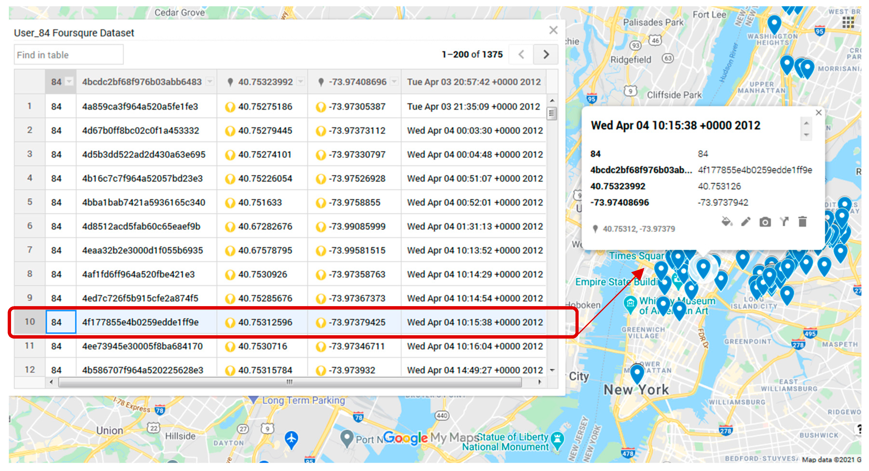
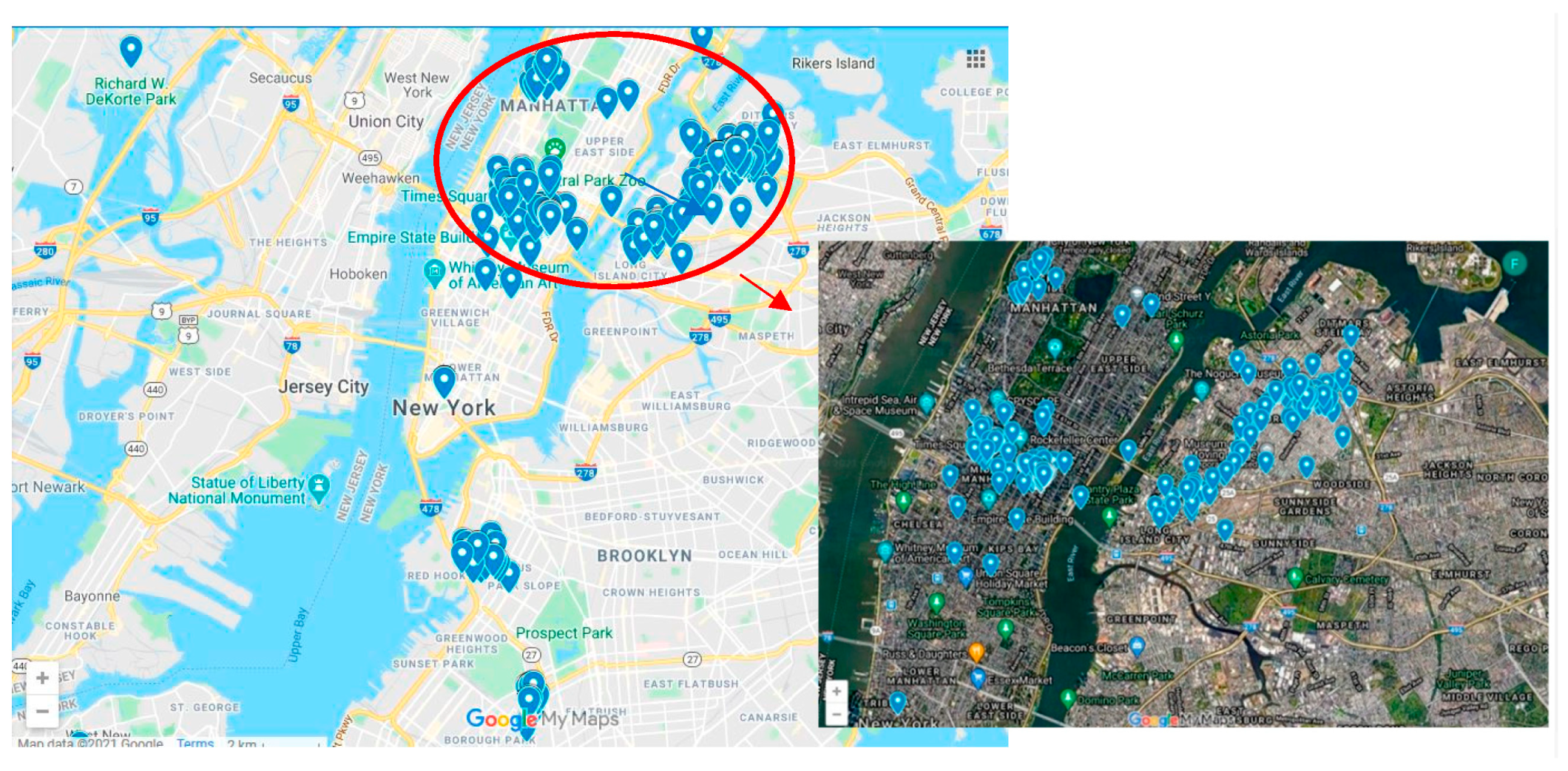
The features of the dataset used in this research are the same for each check-in record in the dataset. These are the user ID, geographic coordinates (longitude and latitude), location ID, and timestamp, which are considered to be static CIs of the movement path. For example, the features of the 1811th check-in of the user with ID 2 in the Gowalla dataset and the features of the 10th user location record with ID 84 in the Foursquare dataset displayed on the map through the Google Map service, which is shown in Figure 1 and Figure 2.

Moreover, the features of the time interval and the geographical distance between two consecutive check-ins are considered as dynamic CI of the movement trajectory.

In this research, we tried to simultaneously compare the effect of timestamp features, time interval, and geographical distance between two consecutive check-ins on the efficiency of the model. To pay attention to the effect of these features in the proposed model, three separate attention gates were used. In the first mode, the effect of all three features on the efficiency of the model was investigated together, and in the second through a fourth mode, the effect of the timestamp, geographical distance, and time interval was investigated by removing each of the attention gates in the model. The results of the experiments showed that the effect of geographical distance on increasing the efficiency of the model was greater than that of timestamp and time interval.

The primary notations utilized herein are listed in

Table 2. Notations and descriptions.

Notation	Description
u, l, v, t	user, location (longitude and latitude), venue or POI, timestamp
lat v, lng v	POI v’s latitude and longitude (geographical coordinates)
cu, v, t	user u-recorded check-in in POI v and timestamp t
Δg, Δt	geographical distance and time interval between two successive check-ins
Su	a set of all user u-generated check-ins
Us, V, T	set of users, POIs, and timestamps
vτu	POI visited by user u at timestamp $\mathsf{\tau }$
tτu, gτu	vector representations of time interval and geographical distance
tru	a sequence of chronologically ordered check-ins linked to u
ϕu, ϕv, ϕt	the latent factors of user u, POI v, and timestamp t
$\hat{\mathrm{h}}$, h	the hidden and candidate states of the EAGRU
zr, rr	update and reset gates of GRU
$\mathsf{\sigma }$	sigmoid function

.

3.2. The MF Method in the CF Approach

The goal of the CF method is to find patterns in a user’s past actions and make predictions for that user based on the preferences of other users [34]. Memory-based, model-based, and hybrid CF algorithms are used in this technique [19,35]. Through the use of memory-based algorithms and a similarity measure or some unique relationships, the target user’s preferences can be predicted by combining the scores of similar individuals, or POIs. Using model-based algorithms that calculate preferences that demonstrate the probability of different POIs being visited, users are recommended particular POIs [34]. MF and Bayesian probabilistic modeling are both included in this method [11]. Memory-based and model-based CF algorithms are combined in hybrid algorithms [35].

MF is the most commonly used model-based CF algorithm in recommender systems [11]. The MF method has been found to be the most precise approach to reducing high sparsity levels in recommendation system databases. In general, MF models map both items and users to a joint latent factor space of dimensionality d, where U-I interactions can be modeled as inner products. The item in the successive POI recommendation is the same POI or venue that the user chose during check-in. As a result, each venue v has a vector q_v ∈ R^d, while each user u has a vector p_u ∈ R^d.

It is worth mentioning, in particular, matrix-factorization-based (MF-based) approaches aim to approximate the matrix R by finding a decomposition of d into two lower-dimensional matrices, namely the latent factors of users (p_u) and venues (q_v). In other words, MF models map both users and venues to a joint latent factor space of dimensionality d, where user–venue interactions are modeled as inner products in that space (R^d). Accordingly, each venue v is associated with a vector q_v ∈ R^d, and each user u is associated with a vector p_u ∈ R^d [34,36].

The elements of q_v for a given venue v measure the degree to which the venue possesses negative or positive factors. The elements of p_u, for a given user u, measure the user’s interest level in venues that score well on the corresponding factors, which can be negative or positive. The obtained dot product, q_v^Tp_u, depicts the user’s u-venue v interaction—the overall interest of the user in the venue’s features. This comes close to how user u has rated venue v, r_uv, yielding the following estimate:

$${\hat{\mathrm{r}}}_{\mathrm{uv}}={\mathrm{p}}_{\mathrm{u}} {\mathrm{q}}_{\mathrm{v}}{}^{\mathrm{T}}$$

(1)

The goal is to minimize the loss function or prediction error in Equation (2), in which K is the set of (u, v) pairs of known ratings [34,36].

min∑_{(u,v)ϵ k} (r_uv − p_u q_v^T)²

(2)

Several methods [36,37] have been introduced to extend MF using RNN models to capture users’ dynamic preferences from a check-in sequence. MF was used to rank the successive POI for a user in our proposed architecture’s output layer. Our proposed EAGRU model is presented in the following section.

3.3. Recurrent Models in Deep Learning

The principal problem with the successive POI recommendations is the joint and efficient learning of user POI preferences as well as the sequential correlations between check-ins [4]. This problem is solved by utilizing hidden states to learn the sequential pattern of an input sequence [11,12,17,22]. Hidden states record the input sequence’s CI, or the sequential pattern.

As a result of the problems with exploding and vanishing gradients in RNN, it cannot capture long-term preferences [10,11]. Long short-term memory (LSTM) is suggested as a solution to these issues. This model employs a gate mechanism to capture long-term preferences [4,38,39]. Every LSTM block also has a cell state c_t as well as a hidden state h_t, which are used in an RNN. In addition, three gates control the information flow between LSTM cells: the input gate, the forget gate, and the output gate [16]. Because LSTM comprises three gates, it is slower to train and requires a lot of data. To address these issues, GRU was proposed [3,19,38]. In the GRU network, there is a reset gate and an update gate that handles each hidden state’s update degree, determining which information is required to be passed to the next state and which does not [22].

GRU only has two gates: the reset and update gates. When less training data exist, the GRU-based model is faster to train and outperforms the LSTM. GRU’s gates control each hidden state’s update degree, determining which data must be passed to the next state and which does not [11,22].

GRU computes the hidden state h_τ at a certain time $\mathsf{\tau }$ using the outputs of the update gate z_τ, the reset gate r_τ, the current input x_τ, the previously hidden state h_τ−1, and the reset gate, and calculates $\hat{\mathrm{h}}$ _τ and h_τ as follows:

z_τ = σ(W_zx_τ + U_zh_τ−1 + b_z)

(3)

r_τ = σ(W_rx_τ + U_rh_τ−1 + b_r)

(4)

ĥ_τ = tanh(Wx_τ + U (r_τ⊙ h_τ−1) + b_h)

(5)

h_τ =(1 − z_τ) ⊙ h_τ−1 + z_τ⊙ ĥ_τ

(6)

where ⊙ represents an elementary multiplication operation. Moreover, W and U denote weight matrices for network training. Here, a feed-forward neural network was applied to compute the alignment function so that a GRU model could be developed, which was inspired by [11,22]. Two attention gates were also proposed based on time intervals and the geographical distance between two successive check-ins.

4. Description of the Proposed Flexible Model

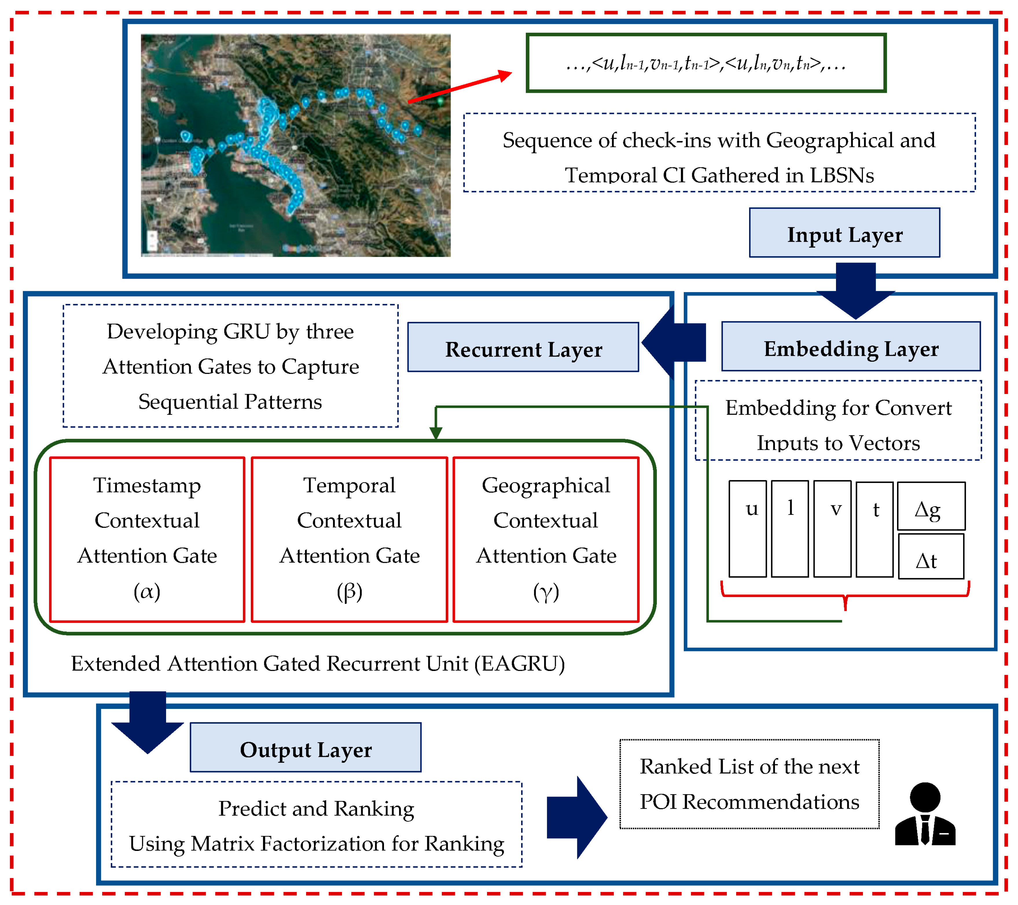
As mentioned above in Section 1, we proposed the EAGRU architecture in order to separately consider the influence of geographical and temporal CI on the next location prediction. The proposed architecture is depicted in Figure 3. Our proposed model architecture consists of input, output, embedding, and recurrent layers.

It should be noted that even though the authors in [3,11,22] also showed how their model grew from the GRU model using the gating mechanism, our proposed architecture is different in how the equations of the gates added to the GRU model are defined and how they affect the basic reset and update gates of the model as well as the hidden layer of the GRU.

4.1. The EAGRU Model Layers

The model inputs, including CI from user check-ins, are stored in the input layer. The proposed model includes a timestamp, user ID, geographical coordinates (longitude and latitude), and venue ID as CI. In addition, transition CI (e.g., the time interval (Δt) and geographical distance (Δg) between two successive check-ins) is provided. In the EAGRU model’s recurrent layer, transition CI is focused on in two proposed gates. The time interval and geographical distance are calculated in this layer as a result. Assuming a user u, a venue v₁, and a time t^τ at timestep τ, the time interval and geographical distance between the given venue v₁ and the venue v₂ visited previously at timestep τ − 1 are computed as Δt^τ = t_τ − t_τ−1 and Δg^τ = dist(lat v₁, lng v₁, lat v₂, lng v₂), respectively (Equation (7)) (Equation (7) is developed using the scikit-learn library, which is available at https://scikit-learn.org, (accessed on 2 October 2022)). The angular distance between the two given points over the surface of a sphere is known as the Haversine distance. The latitude is the first coordinate of each point, and the longitude is the second, measured in radians. With this in mind, two data dimensions are required (In general, the following equation is used to calculate the Haversine distance between samples in X and Y (x₁ and x₂ and y₁ and y₂ are the latitude and longitude of X and Y, respectively)).

D(x,y) = 2* arcsin[√(sin² ((x₁ – y₁)/2) + cos(x₁)cos(y₁) sin² ((x₂ – y₂)/2))]

(7)

Before going to the recurrent layer, the embedding layer is utilized to embed inputs from a sequence of check-ins. Users, POIs (or venues), and time latent factors are generated in this layer as ϕu_i ∈ U, ϕv^τ_i ∈ V, and time ϕt^τ ∈ T, respectively. Moreover, $\mathsf{\theta }$_e = {U, V, T} implies the embedding layer’s set of parameters. The venue ϕv^τ_j and the given time ϕ_t^τ latent factors, as well as the contextual transition features (Δg^τ and Δt^τ), are then passed to the recurrent layer for EAGRU training.

The GRU model was built with two attention gates in the recurrent layer. The present research proposes three attention gates, according to Manotumruksa et al. [11] and Kala et al. [22]: timestamp attention gate (α), temporal attention gate (β), and geographical attention gate (γ).

The input of β, which is the time interval between two successive check-ins, was used to specify more important time intervals in the sequence of historical check-ins of a user. The input of γ is the geographical distance between two successive check-ins applied to specify a more important geographical distance in the sequence of historical check-ins of a user. In other words, they regulate the impact of the earlier recurrent unit’s hidden state based on time intervals and geographical distances between check-ins. It is worth noting that CI affects users’ dynamic preferences differently. This layer’s output is the recurrent unit’s hidden state at timestamp τ, h_τ, as defined below:

h_τ = f (ϕv^τ_j, ϕt^τ,Δt^τ,Δg^τ;θ_r)

(8)

The following is a description of how to extend the traditional GRU to include absolute and CI. Considering the user’s check-in sequence Su and the user’s dynamic preference at timestamp τ, to estimate the hidden state h_τ, the update (z_τ) and reset r_τ) gates in the GRU model are used as follows:

z_τ = σ(W_zϕv^τ_j + U_zh_τ−1 + b_z)

(9)

r_τ = σ(W_rϕv^τ_j + U_rh_τ−1 + b_r)

(10)

ĥ_τ = tanh(Wϕv^τ_j + U (r_τ⊙ h_τ−1) + b_h)

(11)

h_τ= (1 − z_τ) ⊙ h_τ−1+ z_τ ⊙ ĥ_τ

(12)

In the above equations, ϕv^τ_j represents the venue’s latent factor visited by the user at timestamp $\mathsf{\tau }$. In addition, tanh() and $\mathsf{\sigma }$() denote the hyperbolic tangent and sigmoid functions, respectively. Moreover, U implies a recurrent connection weight matrix used to capture sequential signals between every two neighboring hidden states, namely h_τ and h_τ−1. This is performed by employing $\odot$, which indicates the element-wise product. In addition, W and b indicate the transition matrix between the venues’ latent factors and corresponding biases, respectively. Furthermore, θ_r = {W, U, b} represents the set of recurrent layer’s parameters.

The relevant CI must be examined separately to model the users’ check-ins in sequential order effectively. To address this problem, this study proposed gates, α, β, and, γ, which are attention gates that take into account the timestamp (ϕt^τ), time interval (Δt^τ), and geographical distance (Δg^τ) between two check-ins separately as follows:

α = σ(W_α,h h_τ−1 + W_α,ts ϕt^τ + b_α)

(13)

β = σ(W_β,h h_τ−1 + W_β,te Δt^τ + b_β)

(14)

γ = σ(W_γ,h h _τ−1 + W_γ,ge Δg^τ + b_γ)

(15)

When there is a short distance between the two check-ins, the impact of the hidden state h is unlikely to decrease if the time interval between them is long. Together, the attention gates α, β, γ, and the reset gate r_τ control the impact of the earlier hidden state step h_τ−1’s. These gates, as well as the traditional GRU’s update and reset gates, are integrated to find the next hidden state.

It should be noted that in our proposed model, the CIs of the movement path, which are the inputs (features), first pass through the attention gates of α, β, and γ before entering the basic gates of GRU. As stated, these CIs include the venue ID, timestamp, time interval, and geographical distance between two consecutive check-ins by the user. The output vectors of each of the α, β, and γ gates are considered as attention coefficients for timestamp, time interval, and geographical distance, respectively. Additionally, the weight vector of the update and reset gates mentioned in Equations (9) and (10) is multiplied by the features (inputs) of the problem. The candidate hidden layer, which according to Equation (8), is a function of the problem inputs, is rewritten using the product of the output vectors of the attention gates (α, β, and γ) and their corresponding features. Therefore, considering the features of the problem, Equations (9)–(11) are updated as Equations (16)–(18). With the proposed gates for the EAGRU architecture, the equations for the traditional GRU are updated as follows:

z_τ = σ[W_z (ϕv^τ_j + (α ⊙ ϕt ^τ) +(β ⊙ Δt^τ) + (γ ⊙ Δg^τ))+ U_z h_{τ −1} + b_z]

(16)

r_τ = σ[W_r (ϕv^τ_j + (α ⊙ ϕt ^τ) + (β ⊙ Δt^τ) + (γ ⊙ Δg^τ)) + U_rh_{τ −1} + b_r]

(17)

ĥ_τ = tanh[W ϕv^τ_j + (α ⊙ ϕt ^τ) + (β ⊙ Δt^τ) + (γ ⊙ Δg^τ)) + U (r_{τ ⊙} h_τ−1) + b_h]

(18)

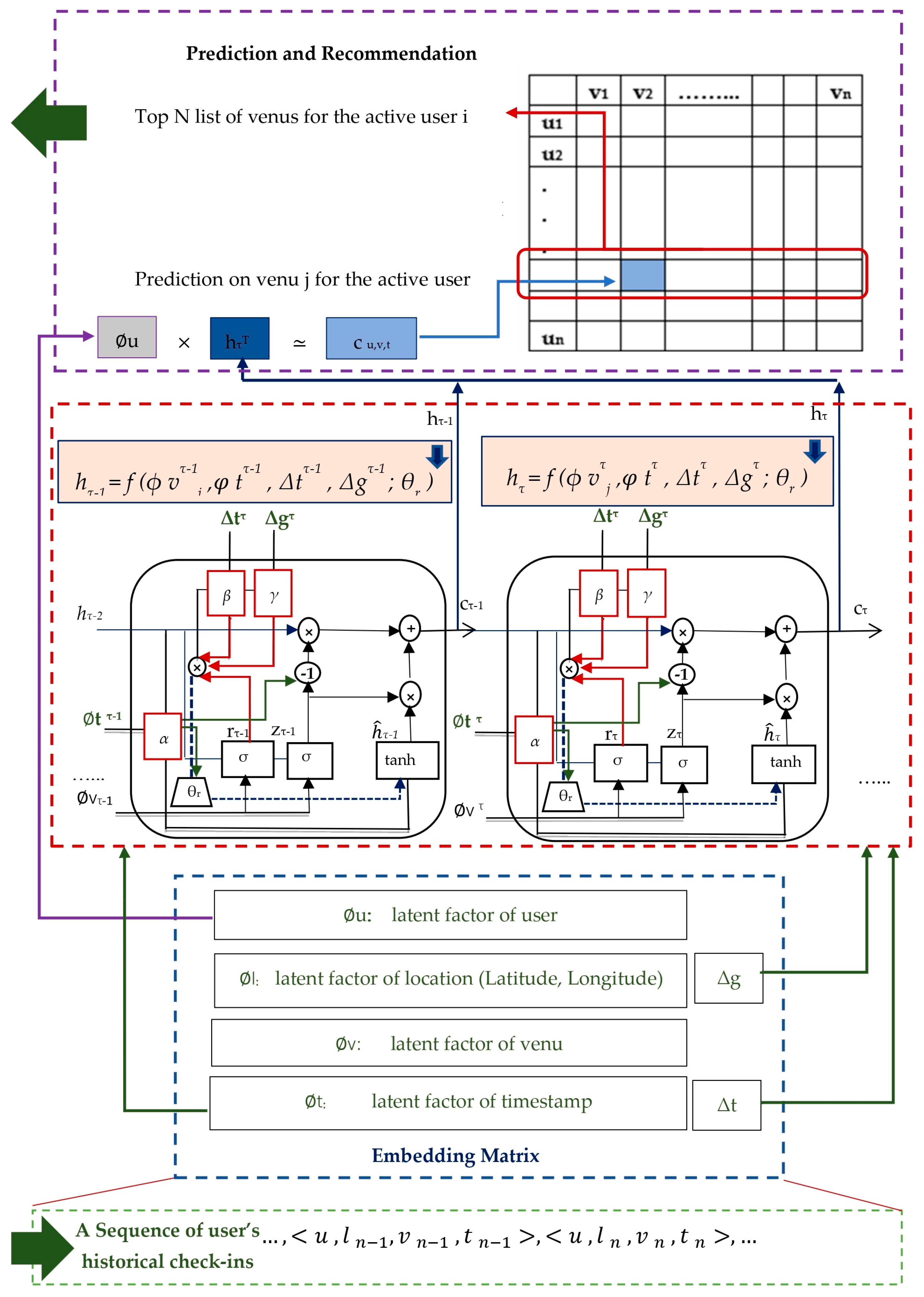
The hidden state h_τ is updated in the following steps, and it is the recurrent unit’s output at timestamp $\mathsf{\tau },$ as previously stated. The block diagram of the EAGRU recurrent layer with the three contextual attention gates is shown in Figure 4.

In the output layer of the EAGRU architecture, inspired by the assumption of the MF method in CF approaches, a ranked list of POI recommendations was provided for each user. It should also be noted that, in the next POI recommendations based on the MF approach, recommendations are mainly derived from a dot product of the latent factors of users U ∈ R^|U|×d and venues V ∈ R^|V|×d where d is the number of latent dimensions (i.e., $\hat{\mathrm{c}}$_i,j = ϕu_i ϕv_j^T) and ϕu_i and ϕv_j denote the latent factors of user i and venue j, respectively [11,21]. In the output layer, the preference of user u on venue v at timestamp $\tau$ is estimated using Equation (19):

ĉ_u,v,t = ϕu_u h^τT

(19)

According to previous studies [11,22,37,40], pairwise loss functions outperformed classification loss functions in learning patterns from sequential data. They also performed more efficiently in network training of recurrent-based recommender systems. According to [11,37,40], the pairwise BPR can estimate the recurrent and embedding layer parameters as well as the probability distribution across all venues considering the hidden state h^τ. The illustration of our proposed model with four layers is shown in Figure 5.

4.2. Developing the EAGRU Model

In this study, we aimed to compare the efficacy of geographical and temporal CI from check-in data in order to predict the location of LBSN users by changing the attention gates in the EAGRU architecture’s recurrent layer. Therefore, considering the main architecture (i.e., EAGRU), four types of architecture were proposed in this research: The first state includes three attention gates in the recurrent layer of the EAGRU architecture to consider the timestamp, geographical distance, and time interval between two successive check-ins. The second state includes two attention gates in the recurrent layer of the EAGRU architecture to consider the time interval and the time geographical distance between two successive check-ins. This removes α gate from our model and the presence of β and γ gates in the model. In this state, the Equations (16)–(18) are rewritten as follows:

z_τ = σ[W_z(Øv^τ_j + ϕt ^τ + (β ⊙Δt^τ) + (γ ⊙ Δg^τ)) + U_z h_{τ −1} + b_z]

(20)

r_τ = σ[W_r (Øv^τ_j + ϕt ^τ + (β ⊙Δt^τ) + (γ ⊙ Δg^τ)) +Øv^τ_j) + U_rh_{τ −1} + b_r]

(21)

ĥ_τ = tanh[W(Øv^τ_j + ϕt ^τ + (β ⊙Δt^τ)+(γ ⊙ Δg^τ))+ Øv^τ_j + U (r_τ ⊙ h_τ−1) + b_h]

(22)

The third state includes two attention gates in the recurrent layer of the EAGRU architecture to consider the timestamp and the time interval between two successive check-ins. This removes the γ gate from our model and the presence of α and β gates in the model. In this state, the Equations (16)–(18) are rewritten as follows:

z_τ = σ[W_z (Øv^τ_j + (α ⊙ ϕt ^τ) + (β ⊙ Δt^τ) + Δg^τ) + U_z h_{τ −1} + b_z]

(23)

r_τ = σ[W_r (Øv^τ_j + (α ⊙ ϕt ^τ) + (β ⊙ Δt^τ) + Δg^τ) + U_rh_{τ −1} + b_r]

(24)

ĥ_τ = tanh[W Øv^τ_j + U (r_τ ⊙ h_τ−1) + W((α ⊙ ϕt ^τ) + (β ⊙ Δt^τ) + Δg^τ) + b_h]
ĥ_τ = tanh[W(Øv^τ_j +(α ⊙ ϕt ^τ) + (β ⊙ Δt^τ) + Δg^τ) + U (r_τ ⊙ h_τ−1) + b_h]

(25)

The fourth state includes two attention gates in the recurrent layer of the EAGRU architecture to consider the timestamp and geographical distance between two successive check-ins. This removes the β gate from our model and the presence of α and γ gates in the model. In this state, the Equations (16)–(18) are rewritten as follows:

z_τ = σ[W_z (Øv^τ_j + (α ⊙ ϕt ^τ) + Δt^τ + (γ ⊙ Δg^τ))+ U_z h_τ−1 + b_z]

(26)

r_τ = σ[W_r (Øv^τ_j + (α ⊙ ϕt ^τ) + Δt^τ + (γ ⊙ Δg^τ)) + U_rh_τ−1 + b_r]

(27)

ĥ_τ = tanh[W (ϕv^τ_j + (α ⊙ ϕt ^τ) + Δt^τ +(γ ⊙ Δg^τ)) +U (r_τ ⊙ h_τ−1) + b_h]

(28)

4.3. Network Training

This research employed datasets made up of sampled triplets with one user and two POIs, one of which is positive (i.e., visited) and the other is negative (i.e., unvisited). As previously mentioned, the pairwise BPR was used to learn the embedding and recurrent layer parameters ($\mathsf{\Theta }$ = {$\mathsf{\theta }$_e,$\mathsf{\theta }$_r}) in this study. BPR considers the relative prediction order for POI pairs based on the underlying assumption that a user prefers the observed POIs over all unobserved ones [3,4]. EAGRU aims to maximize the probability [3,4,40] at each sequential position k in the BPR framework:

P(u, t, v > v’) = 1/(1 + e^−x) (o_u,t,v − o_u,t,v’)

(29)

where v and v′ denote positive (i.e., visited) and negative (i.e., unvisited) POIs, respectively. To solve the network’s objective function for the next POI recommendation, the regularization term and the loss function must be integrated, as shown below [40]:

$$\mathrm{J}=-{{\displaystyle \sum }}_{\left(\mathrm{v}, \mathrm{v}\prime \right)}\mathrm{lnP}(\mathrm{u},\mathrm{t},\mathrm{v}> \mathrm{v}\prime )+\mathsf{\lambda }/2 \left|\left|\mathsf{\Theta }\right|\right|{ }^2$$

(30)

where λ indicates the regularization power, and $\mathsf{\Theta }$ denotes the setoff parameters. Following [11] and [22], the dimensions of the EAGRU architecture’s hidden layers h_τ and latent factors d (d = 10) are set across the two datasets. Moreover, all the recurrent and embedding layers’ parameters can be initiated randomly using a Gaussian distribution. At the beginning, the batch size and learning rate are set to 256 and 0.001, respectively. The parameters of the model are optimized using the Adam optimizer. The EAGRU’s recurrent layer’s parameter set includes U, W, and b for the reset and α and β update gates, respectively. The EAGRU model produces a collection of scores for POIs that are similar to their chances of being the successive POI in each sequence. A summary of the learning algorithm of EAGRU is provided as Algorithm 1:

Algorithm 1: Training of EAGRU.
Input: Set of users Us and set of historical check-in sequences Su
	//construct training instances
1.	Initialize Du = ∅, Du is a set of check-in trajectory samples combined with negative POIs of u
2.	For each user u $\in$ Us do
3.	For each check-in sequence Su = {st1u, st2u,…, stnu } do
4.	Get the set of negative samples $\mathrm{v}\prime$
5.	For each check-in activity in Su do
6.	Compute the embedded vector vτu
7.	Compute the geographical contexts vector gτu
8.	Compute the temporal contexts vector tτu
9.	End for
10.	Add a training instance ({vτu, gτu, tτu },{$\mathrm{v}\prime$}) into Du
11.	End for
12.	End for
	//train the model
13.	Initialize the parameter set Θ
14.	While (exceed (maximum number of iterations) == FALSE) do
15.	For each user u in U do
16.	Randomly select a batch of instances Dnu from Du
17.	Find Θ minimizing the objective Equation (29) with Dnu
18.	End for
19.	End While
20.	Return the set of parameters Θ

5. Experimental Results

The experimental setup and empirical findings of this study are presented in this section. To validate the proposed method’s efficiency, empirical experiments were carried out on two public datasets in LBSNs. These experiments were designed to respond to the following research questions to address the issues raised in Section 1:

• RQ1: How can the EAGRU architecture be developed to compare the efficacies of geographical and temporal CI associated with the sequence of check-ins for location prediction?
• RQ2: Which CI, geographical distance or time interval, has the greatest effect on location prediction accuracy?
• RQ3: Does EAGRU, which leverages multiple types of CI, improve prediction by applying additional attention gates or, does it outperform the previous methods?

In this study, the tests were carried out to assess two publicly available LBSN datasets: Gowalla (https://snap.stanford.edu/data/loc-gowalla.html) accessed on 10 September 2022 and Foursquare (https://sites.google.com/site/yangdingqi/home/foursquare-dataset accessed on 1 August 2022). To reduce data sparsity and cold start problems, users with fewer than ten check-ins and POIs selected fewer than ten times were removed from the two datasets, as recommended by [11]. The statistics from the two datasets are summarized in

Table 3. Statistics of the two datasets.

Dataset	#Users	#Check-Ins	#POIs	Density
Gowalla	1047	614,340	5011	0.1170
Foursquare	615	108,195	19,245	0.0091

. A check-in record in this study is quadrupled and includes a user, a check-in timestamp, geographical check-in coordinates, and a location ID or POI. User sequences were created from the check-in history in the two datasets. For two datasets, the density formula is:

Density = (|check-ins|)/(|users| × |POIs|)

(31)

It should be noted that data density, according to Equation (31), is the ratio of the number of check-ins of users to the product of the number of users and the number of places visited by users in the dataset [41]. Dataset density can be a measure of the amount of the dataset selected for experiments from the entire dataset.

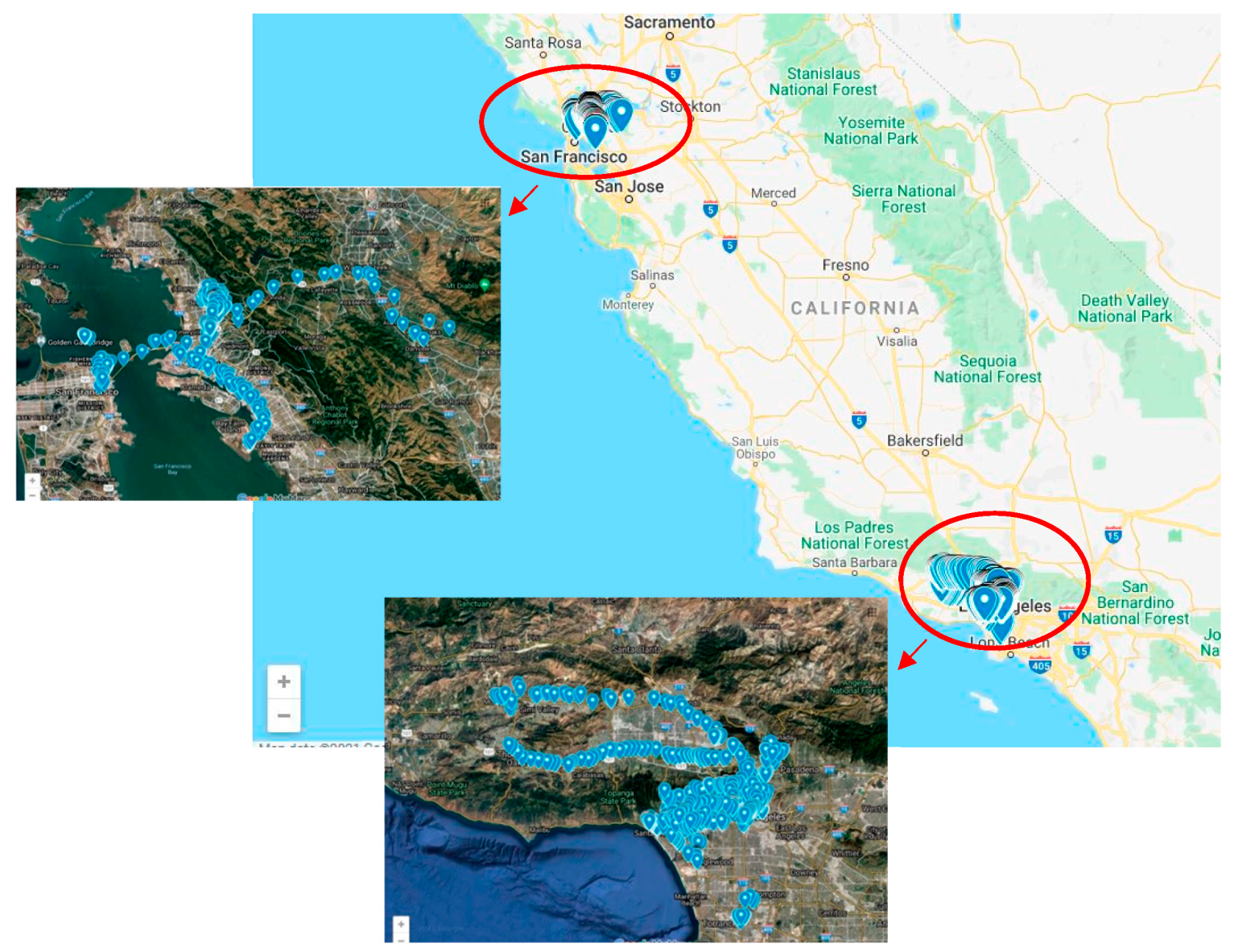
A visualization of the data in each dataset on the map, which is actually the distribution of the users’ positions, was performed in order to display the data more clearly. For this purpose, we selected a user from each of the Gowalla and Foursquare datasets and displayed the sequence of recording of his/her positions on the map through the Google Map service, which is shown in Figure 6 and Figure 7.

Figure 6 shows the check-ins of the user with ID 2 in the Gowalla dataset. The total number of check-ins for this user is 2100, and this sequence of check-ins includes 1870 places (POIs) that were visited by the user.

Figure 7 shows the check-ins of the user with ID 84 in the Foursquare dataset. The total check-ins for this user were 1376, and this sequence of checks included 334 POIs selected by the user. Figure 6 also shows the features of recording the 10th position of this user in the table.

Based on previous studies [11,22], the leave-one-out cross-validation methodology was used to assess the efficiency of the proposed EAGRU architecture: Each user’s most recent check-in was used as the basis, and 100 POIs that had not been visited previously were selected at random. They were the testing set, while the rest of the check-ins were the training set. The EAGRU’s task was to rank those 100 venues as preferred contexts for each user (based on timestamp, geographical distance, and time interval), with the most recent, ground truth check-in being ranked first. Following [11,22], the dimensions of the proposed EAGRU architecture’s hidden layers h_τ and latent factors d (d = 10) were set. As previously stated, the Gaussian distribution [13] was used to randomly initialize the parameters of the recurrent layer, and the Adam optimizer [42] was used for parameter optimization due to its faster convergence than the stochastic gradient descent (SGD) optimization, which sets the learning rate in each iteration. To avoid overfitting, the batch size and the dropout rate were set to 256 and 0.2, respectively.

To compare the efficacy of the temporal and geographical CI of check-in data in location prediction for LBSN users, we designed four sets of experiments obtained by changing the attention gates in our proposed architecture’s recurrent layer. We used the recall metric (Rec@k, k = 5, 10) to evaluate the above-mentioned methods’ performance and see if the ground truth location could be found in the top-k recommendation list. Equation (32) [3] defines Recall@ in general:

Recall@k = 1/N ∑ _{(u = 1)}^N((S_u(k)∩V_u)/(|V_u|)

(32)

where S_u(k) indicates the set of top- k POIs recommended for user u, and Vu implies the set of POIs actually visited by user u at the next timestamp in the test set.

5.1. Incorporation of the Four Experiment States

In this research we aimed to predict the location of users using the CI of the user’s movement path in LBSN. The dataset of social networks based on the location investigated in this research was collected using check-ins that users recorded along their trajectory. As mentioned, each check-in includes the user ID, venue ID, geographic coordinates, and timestamp of the check-in, which is the static CI of the user’s movement trajectory. These are also the features used in the tests. Moreover, the time interval and geographical distance between two consecutive check-ins were used as a dynamic CI of the user’s movement trajectory and are important features used in this research. The focus of this article is on the timestamp features, the time interval, and the geographical distance between two consecutive check-ins, and the authors intend to separately investigate the effect of each of these factors in increasing the accuracy of predicting the user’s location.

According to the studies conducted in the past, the effect of the set of effective factors in predicting the location was examined together, and how much each of the CIs separately affects the accuracy of the prediction was not included in the past models. Obviously, by knowing the factors (CIs) that have a greater impact than other factors in predicting the location of users, researchers can provide more effective solutions to improve location-based recommender systems. We consider this issue one of the most important research challenges and took advantage of it as an opportunity to present a preliminary model as well as an innovative design of our experiments.

To do this, we came up with a model that uses the flexibility of the GRU model and its development with the help of three content attention gates for each of the effective factors in predicting the location. This lets us look at the effect of each CI on the movement path separately. In the following, the authors describe how they innovatively designed the experiments on the model in four modes. In the first mode, the whole model was implemented with three attention gates. In the second, third, and fourth modes, the attention gates of each of the effective factors in predicting the location were removed according to the order of the gates (the timestamp, time interval, and geographical distance). This initiative is for the separate investigation of each of the effective factors in predicting the location of people.

The experiments are explained in four states:

First state, the EAGRU model with three contextual attention gates (α, β and, γ);

Second state, the EAGRU model with two contextual attention gates (β and γ);

Third state, the EAGRU model with two contextual attention gates (α and β);

Fourth state, the EAGRU model with two contextual attention gates (α and γ).

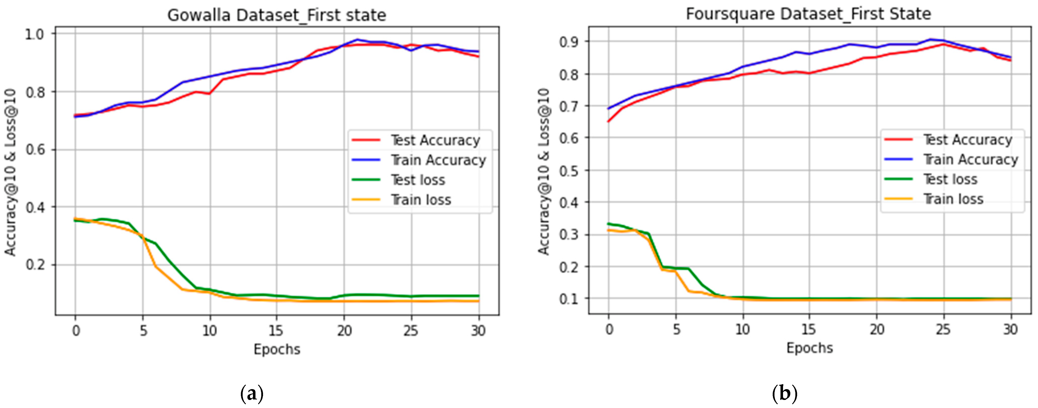
The first state includes three attention gates in the recurrent layer of the EAGRU architecture to consider the timestamp, geographical distance, and time interval between two successive check-ins. This state is our proposed model that is described in Section 4. Training and testing accuracy @10 and loss @10 for the Gowalla and Foursquare datasets vs. epoch in the EAGRU model are shown in Figure 8.

According to Figure 8, in the first state of the tests, in the 30 epochs of the train and test processes, the highest Recall@10 for prediction in the Gowalla dataset was observed in the 21st and 22nd epochs, respectively. In the Foursquare dataset, the highest Recall@10 for prediction was observed in the 25th epoch, and in each of the datasets, the prediction efficiency decreased from the mentioned periods onward. Moreover, in these 30 epochs, the lowest amount of loss was observed in the processes of training and testing in the Gowalla dataset in the 22nd and 18th epochs and in the 18th and 20th epochs in the Foursquare dataset. In each of the datasets, from the mentioned epochs onward, the error rate increased.

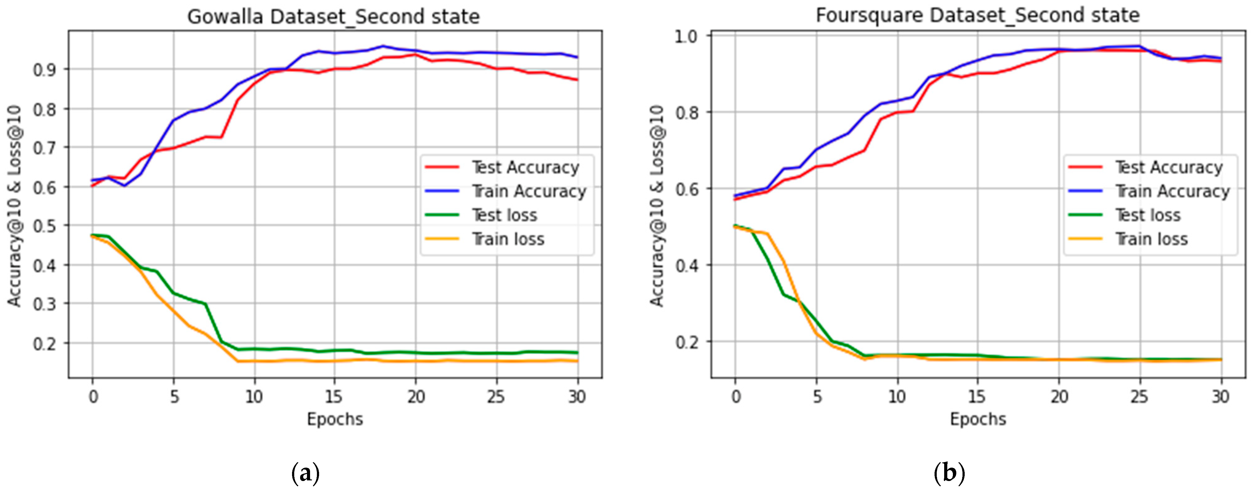
The second state includes two attention gates in the recurrent layer of the EAGRU architecture to consider the timestamp and the time interval between two successive check-ins. Training and testing accuracy @10 and loss @10 for the Gowalla and Foursquare datasets vs. epoch in the EAGRU model in the second state of experiments are shown in Figure 9.

According to Figure 9, in the second state of the tests, in the 30 epochs of the training and testing processes, the highest accuracy@10 for prediction in the Gowalla dataset was observed in the 18th and 20th epochs, respectively. In the Foursquare data, the highest accuracy@10 for prediction was observed in the 19th and 21st epochs, respectively. In each of the datasets, the prediction efficiency decreased from the mentioned periods onward. Moreover, in these 30 epochs, the lowest amount of loss was observed in the processes of training and testing in the Gowalla dataset in the 19th and 20th epochs, respectively, and in the Foursquare dataset in the 23rd and 20th epochs, respectively, and in each of the datasets of the mentioned epochs, the error rate increased from then.

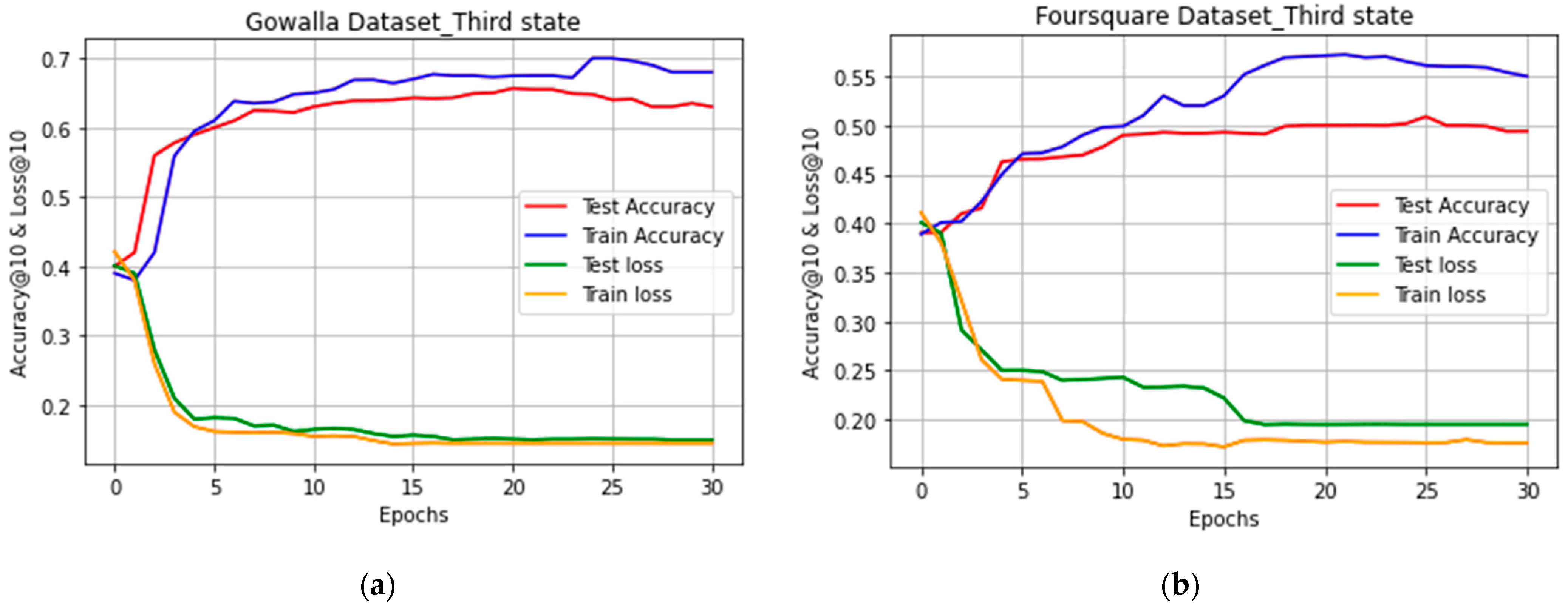
The third state includes two attention gates in the recurrent layer of the EAGRU architecture to consider the timestamp and the time interval between two successive check-ins. Training and testing accuracy @10 and loss @10 for the Gowalla and foursquare datasets vs. epoch in the EAGRU model in the third state of experiments are shown in Figure 10.

According to Figure 10, in the third state of the tests, in the 30 epochs of the train and test processes, the highest accuracy@10 for prediction in the Gowalla dataset was observed in the 24th and 20th epochs, respectively. In the Foursquare data, the highest accuracy@10 for prediction was observed in the 21st and 25th epochs, respectively. In each of the datasets, the prediction efficiency decreased from the mentioned periods onward. Moreover, in these 30 epochs, the lowest amount of loss was observed in the processes of train and test in the Gowalla dataset in the 14th and 16th epochs, respectively, and in the Foursquare dataset in the 15th and 17th epochs. In each of the datasets for the mentioned epochs, the error rate increased from then.

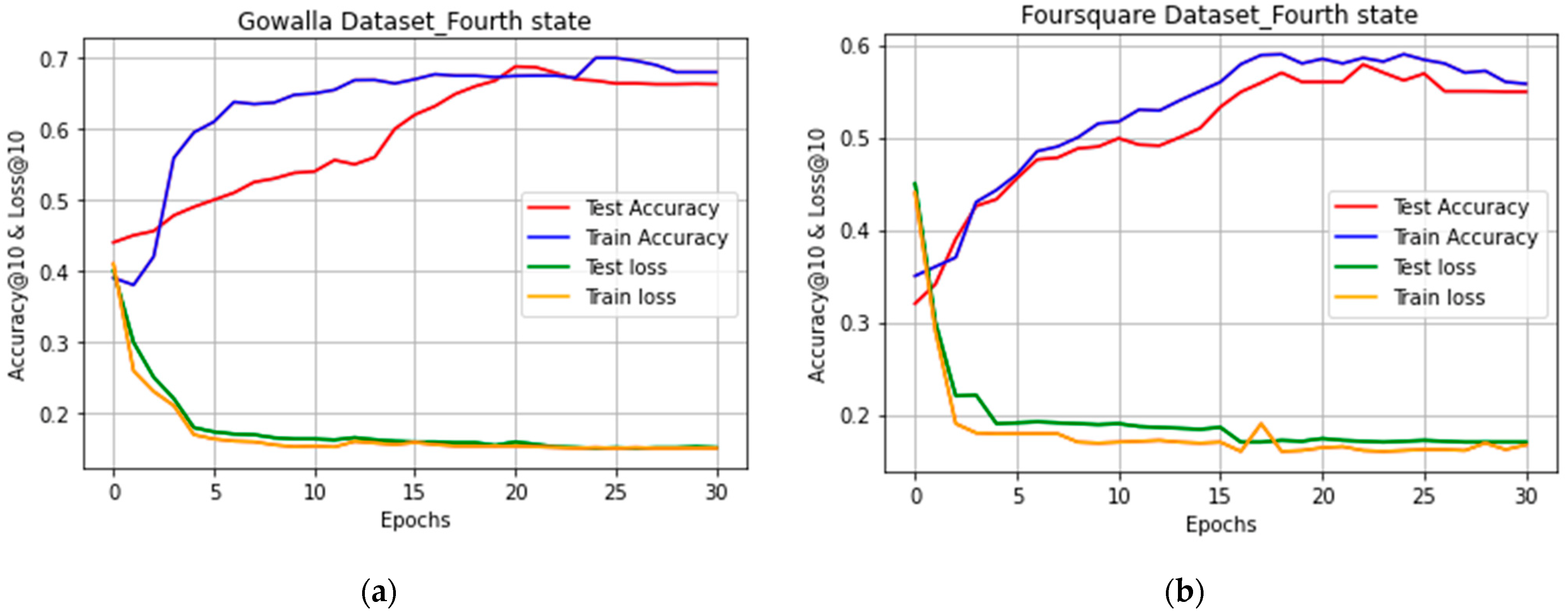
The fourth state includes two attention gates in the recurrent layer of the EAGRU architecture to consider the timestamp and geographical distance between two successive check-ins. Training and testing accuracy @10 and loss @10 for the Gowalla and foursquare datasets vs. epoch in the EAGRU model in the fourth state of experiments are shown in Figure 11.

According to Figure 11, in the fourth state of the tests, in the 30 epochs of the training and testing processes, the highest accuracy@10 for prediction in the Gowalla dataset was observed in the 24th and 20th epochs, respectively. In the Foursquare data, the highest accuracy@10 for prediction was observed in the 17th and 22nd epochs, respectively. In each of the datasets, the prediction efficiency decreased from the mentioned periods onward. Moreover, in these 30 epochs, the lowest amount of loss was observed in the processes of training and testing in the Gowalla dataset in the 23rd and 24th epochs, respectively, and in the Foursquare dataset in the 16th epoch. In each of the datasets for the mentioned epochs, the error rate increased from then.

The results of the comparison of the four states of experiments are shown in

Table 4. A comparison among four sets of experiments.

Recall
States	@k	Gowalla	Foursquare
First	5	0.7945	0.7033
	10	0.9063	0.8814
Second	5	0.7854	0.8312
	10	0.8940	0.9301
Third	5	0.4072	0.4178
	10	0.4275	0.4383
Fourth	5	0.5098	0.4987
	10	0.5451	0.5236

. It should be noted that Table 4 is presented with the aim of expressing the efficiency of each of the contextual attention gates. As stated in Section 4.2 of the original manuscript, the first state of the experiments was performed with the presence of three defined attention gates, and the second to fourth states were performed by removing the gates of timestamps, geographical distance, and time interval, respectively. The reduction in the value of the evaluation metric in each state shows the importance of the presence of the removed attention gate. As the evaluation metric decreases, it indicates that the attention gate removed from the model has a more significant impact on modeling the relationship between users’ check-ins and predicting their location.

Table 5. The performance of each CI attention gate.

			Percentage of Change
States	Removed Attention Gates	K	Gowalla (%)	Foursquare (%)
Second	α	5	−01.15	+18.19
		10	−01.36	+05.53
Third	γ	5	−48.75	−40.59
		10	−52.83	−50.27
Fourth	β	5	−35.83	−29.09
		10	−39.85	−40.59

displays the results of three states of experimentation on the influence of factors on predicting the user’s location. As can be seen, the removal of any attention gate in the second to fourth states of the experiments caused a change in the prediction accuracy. In other words, the larger the accuracy reduction, the greater the significance of the removed attention gate or, more generally, the CI associated with that attention gate.

In our set of experiments, the largest performance reduction was related to the γ gate; that is, the removal of the attention gate related to the CI of the geographical distance between consecutive users’ check-ins, and it is presented in bold as follows in Table 5. After the γ gate, the β and alpha α, respectively, have a significant impact in modeling the relationships between check-ins in predicting the user’s location.

5.2. Other Methods in Comparison

An evaluation of the EAGRU’s performance in predicting locations was conducted by comparing five of the most up-to-date methods. These models can be summarized as follows:

GT-SEER: The authors of [25] proposed the Geo-Temporal Sequential Embedding Rank (GT-SEER) approach using the Skip-Gram model for temporal POI embedding and BPR for pairwise POI ranking combined in a unified framework.

LSTPM: The authors of [20] proposed long- and short-term preference modeling (LSTPM) for the next POI recommendation, comprising a geo-dilated RNN for short-term preference learning and a non-local network for long-term preference modeling. They developed a geo-dilated RNN to take advantage of the geographical relations among non-successive POIs and overcome the limitations of RNNs in short-term user preference modeling.

ASTEM: The authors of [27] introduced the Attentive Spatio-Temporal Neural Model (ASTEM), a deep LSTM RNN model with an attention/memory mechanism for the sequential POI recommendation problem that captures both the sequential and temporogeographical features in its learned representations.

MCI-DNN: A multi-context integrated deep neural network model (MCI-DNN) was proposed by [21] for determining the next location. They integrated sequence/input contexts and user preferences into a unified framework. Their proposed model added many elements to the RNN model that could be found in each of the hidden layers. This was carried out to capture location-related context.

CARA: The authors of [11] proposed the Contextual Attention Recurrent Architecture (CARA) model, which captures users’ dynamic preferences by combining feedback sequences with CI linked to the sequences.

5.3. Results and Discussion

Table 6. A comparison between different methods for recommendation performance.

Methods	Recall
	Gowalla		Foursquare
	@5	@10	@5	@10
GT-SEER	0.0650	0.1200	0.1401	0.2001
LSTPM	0.2021	0.2510	0.3372	0.4091
ASTEM	0.1440	0.2660	0.3280	0.4140
MCI-DNN	0.3665	0.4396	0.2918	0.4006
CARA	-	0.7385	-	0.8851
EAGRU	0.7945	0.9603	0.7033	0.8814

compares the results of the five methods on the two datasets in terms of recommendation.

When the experimental results of the models in Table 6 were compared, it was discovered that failing to use RNN models (i.e., the GT-SEER model) reduced the prediction evaluation metric. This result highlights the importance of employing an RNN approach when modeling historical user check-in relationships. The LSTPM model simply utilizes the LSTM model for location recommendation, and it has a lower prediction evaluation metric than the ASTEM, MCI-DNN, and CARA models, despite taking temporal CI into account.

The ASTEM model considers the order in which previously visited venues were visited, and it employs an LSTM model to model the CI surrounding check-ins. The CARA model, which uses the GRU model, has a higher prediction evaluation.

Despite the fact that the MCI-DNN model takes into account GTCI, it does not employ the attention mechanism approach. It, too, employs the RNN model and has a lower evaluation metric than GRU-based models such as CARA. In spite of using the RNN model, the MCI-DNN model has a higher recall metric than the LSTPM model since it incorporates CI separately. However, when compared to the CARA model, it has a lower evaluation metric due to the absence of an attention mechanism. When compared to other models, the CARA model has a higher evaluation result.

It is worth noting that hybrid approaches (RNN, AM, and MF) outperform RNN or AM-based models. This means that having a good network architecture is not enough to achieve good results, and more geographical and temporal CI about human check-in behavior is needed.

Since GTCI is used separately, and RNN, attention, and factoring approaches are employed in combination, the CARA model’s Recall@10 metric is higher than the other compared models. We applied an attention gate to the GRU model to address the check-in timestamp to enhance the prediction performance of the next POI recommendation, which was inspired by the main idea behind this model.

Our proposed model employs two distinct attention gates, α and β, which take into account the time interval and geographical distance between successive check-ins, respectively, and the output of each of them influences the values of the GRU model’s reset and update gates separately. The proposed EAGRU architecture improves the Recall@10 metric, as shown in Table 6.

In response to RQ1, we defined four states that are obtained by changing the attention gates in the recurrent layer of the EAGRU architecture. These gates’ output influences the GRU reset/update gates’ values, and they are in charge of controlling the user’s trajectory data’s GTCI.

In response to RQ2, the experiments are conducted in four states. According to the experimental results in the four states that are shown in Table 5, we understand the CI of geographical distance and time interval are both important in predicting the location of LBSN users, because by removing attention gates related to them from the EAGRU model (third and fourth states), the recall of the prediction decreases. Moreover, according to our experiments, by comparing the third and fourth states, we find that the efficacy of the CI of the geographical distance (geographical CI) is greater than the CI of the time interval (temporal CI), because by removing the geographical distance attention gate (third state), the Recall@5, and @10 decreases more than when the time interval attention gate is removed (fourth state).

In response to RQ3, these results (Table 6) were found by comparing the EAGRU model’s Recall@10 metric with current architectures.

6. Conclusions

In this research, we proposed a novel architecture (that we named the EAGRU model) for the next POI recommendation, and among its advantages are the simplicity of the design and high flexibility for its development in order to consider more CI in the future. The effect of each CI on the user’s trajectory can be tested, and the innovative design of experiments in four states demonstrates the possibility of comparing the effectiveness of each CI in the model’s prediction accuracy. The comprehensive comparative experiments proposed in this study are a significant research innovation not seen in previous studies. Our proposed architecture was presented with the development of the GRU model using three attention gates named α, β, and, γ, in which, respectively, the timestamp, time interval, and geographical distance CI of the user trajectory data are considered separately, and it provides the possibility of examining their separate impact in increasing the forecasting accuracy. Moreover, the development of the model inspired by the AM makes CI more important in modeling sequential user data. POIs were scored to provide recommendations to a user based on his or her historical check-ins. Four comprehensive experiments were performed on two real-world, large-scale datasets, namely, Gowalla [23] and Foursquare [24], which have been widely used in related studies to predict user POI in LBSNs.

The goal was to assess the effectiveness of the geographical and temporal CI contained in check-in data separately in the location prediction of LBSN users. For this purpose, using the flexibility of our model, the experiment was designed in four states, with the second to fourth states executed by removing the α, β, and γ attention gates to determine their effect on the performance of the model. In this set of tests, except for the Foursquare dataset, which had a different behavior due to the different distribution of check-ins and its low density, in the Gowalla dataset, the highest accuracy was in the first state of the tests; that is, when all three attention gates were present in the model.

In the third state of the experiment, by removing the γ gate, which was related to the geographical distance CI, the greatest decrease in efficiency was observed. In the Gowalla dataset, for Recall@5 and @10, the efficiency reduction was 48.75 and 52.83%, respectively, and for the Foursquare dataset, the efficiency reduction for Recall@5 and @10 was 40.59 and 50.27, respectively. This is a sign of the greater effect of the CI of the geographical distance on the accuracy of our model. After that, the effect of the CI of the time interval is important in the prediction accuracy because in the fourth state, in the Gowalla dataset, for Recall@5 and @10, the efficiency reduction was 35.83 and 39.85%, respectively, and for the Foursquare dataset, the efficiency reduction for Recall@5 and @10 was 29.09 and 40.59, respectively. After the CIs of geographical distance and time interval, the CI of timestamp is important in forecasting accuracy because the removal of the attention gate related to it caused a slight decrease in the efficiency of the model. Of course, in the Foursquare dataset, as already said, and contrary to expectations, an increase in the efficiency of the model was observed. In the second state, in the Gowalla dataset, for Recall@5 and @10, the efficiency decreased by 1.15 and 1.36 percent, respectively, and for the Foursquare dataset, the efficiency increased by 18.19 and 5.53 percent.

Therefore according to our experiments, by comparing the third and fourth states, we find that the efficacy of the CI of the geographical distance (geographical CI) is greater than the CI of the time interval (temporal CI), because by removing the geographical distance attention gate (third state), the Recall@5 and @10 decreases more than when the time interval attention gate is removed (fourth state). Furthermore, the results revealed that the performance of EAGRU was higher than that of competitive baseline methods.

The EAGRU architecture could be expanded by adding the influence of each user’s social relationships with other users on LBSNs and even more by employing CI related to check-in data in the future. In future investigations, it may be possible to include additional CI, such as textual and visual information about users’ check-ins and the current weather at the registered location for check-ins. It is also possible to compare the impact of new context with the comprehensive experiments presented in this research. This study could also be applied to a larger scale of geographic prediction, but with more specific context involved, such as electric vehicle (EV) car drivers, and it provides the possibility of further research for those interested in this field. Experiments should be performed to find out more about the effect of data density and its factors, such as the number of check-ins, the number of users, and the number of places visited. Since it was found that geographic CI had a significant effect on performance in this study, this area can be focused on more by conducting experiments related to the distance calculation methods and by determining how the performance changes according to these methods in the future.

References

1. Fan, X.; Guo, L.; Han, N.; Wang, Y.; Shi, J.; Yuan, Y. A Deep Learning Approach for Next Location Prediction. In Proceedings of the 22th IEEE International Conference on Computer Supported Cooperative Work in Design (CSCWD), Nanjing, China, 9–11 May 2018. [Google Scholar]
2. Baral, R.; Li, T.; Zhu, X. CAPS: Context Aware Personalized POI Sequence Recommender System. arXiv 2018, arXiv:1803.01245. [Google Scholar]
3. Liu, C.; Liu, J.; Wang, J.; Xu, S.; Han, H.; Chen, Y. An Attention-Based Spatiotemporal Gated Recurrent Unit Network for Point-of-Interest Recommendation. ISPRS Int. J. Geo-Inf. 2019, 8, 355. [Google Scholar] [CrossRef] [Green Version]
4. Huang, L.; Ma, Y.; Wang, S.; Liu, Y. An Attention-based Spatiotemporal LSTM Network for Next POI Recommendation. IEEE Trans. Serv. Comput. 2019, 14, 1585–1597. [Google Scholar] [CrossRef]
5. Christoforidis, C.; Kefalas, P.; Papadopoulos, A.N.; Manolopoulos, Y. RELINE: Point-of-Interest Recommendations using Multiple Network Embeddings. J. Knowl. Inf. Syst. 2019, 63, 791–817. [Google Scholar] [CrossRef]
6. Yuan, Q.; Cong, G.; Ma, Z.; Sun, A.; Magnenat-Thalmann, N. Time-aware Point-of-interest Recommendation. In Proceedings of the 36th ACM SIGIR Conference on Research and Development in Information Retrieval, Dublin, Ireland, 28 July–1 August 2013. [Google Scholar]
7. Luan, W.; Liu, G.; Jiang, C.; Qi, L. Partition-based collaborative tensor factorization for POI recommendation. IEEE/CAA J. Autom. Sin. 2017, 4, 437–446. [Google Scholar] [CrossRef]
8. Maroulis, S.; Boutsis, I.; Kalogeraki, V. Context-aware Point-of-Interest Recommendation Using Tensor Factorization. In Proceedings of the IEEE International Conference on Big Data, Washington, DC, USA, 5–8 December 2016. [Google Scholar]
9. Gao, Q.; Zhou, F.; Trajcevski, G.; Zhang, K.; Zhong, T.; Zhang, F. Predicting Human Mobility via Variational Attention. In Proceedings of the World Wide Web Conference, San Francisco, CA, USA, 13–17 May 2019. [Google Scholar]
10. Huang, L.; Ma, Y.; Liu, Y.; He, K. DAN-SNR: A Deep Attentive Network for Social-Aware Next Point-of-Interest Recommendation. ACM Trans. Internet Technol. 2020, 21, 1–27. [Google Scholar] [CrossRef]
11. Manotumruksa, J.; Macdonald, C.; Ounis, I. A Contextual Attention Recurrent Architecture for Context-Aware Venue Recommendation. In Proceedings of the 41th International ACM SIGIR Conference on Research & Development in Information Retrieval, Ann Arbor, MI, USA, 8–12 July 2018. [Google Scholar]
12. Yao, D.; Zhang, C.; Huang, J.; Bi, J. SERM: A Recurrent Model for Next Location Prediction in Semantic Trajectories. In Proceedings of the ACM Conference on Information and Knowledge Management, Singapore, 6–10 November 2017. [Google Scholar]
13. Li, J.; Liu, G.; Yan, C.; Jiang, C. LORI: A Learning-to-Rank-Based Integration Method of Location Recommendation. IEEE Trans. Comput. Soc. Syst. 2019, 6, 430–440. [Google Scholar] [CrossRef]
14. Liu, Q.; Wu, S.; Wang, L.; Tan, T. Predicting the Next Location: A Recurrent Model with Geographical and Temporal Contexts. In Proceedings of the Conference on Artificial Intelligence (AAAI), Phoenix, AZ, USA, 12–17 February 2016. [Google Scholar]
15. Zhao, P.; Luo, A.; Liu, Y.; Xu, J.; Li, Z.; Zhuang, F.; Sheng, V.S.; Zhou, X. Where to Go Next: A Spatio-Temporal Gated Network for Next POI Recommendation. IEEE Trans. Knowl. Data Eng. 2020, 34, 2512–2524. [Google Scholar] [CrossRef]
16. Wang, P.; Wang, H.; Zhang, H.; Lu, F.; Wu, S. A Hybrid Markov and LSTM Model for Indoor Location Prediction. IEEE Access 2019, 7, 185928–185940. [Google Scholar] [CrossRef]
17. Zhang, Z.; Li, C.; Wu, Z.; Sun, A.; Ye, D.; Luo, X. NEXT: A Neural Network Framework for Next POI Recommendation. Front. Comput. Sci. 2017, 14, 314–333. [Google Scholar] [CrossRef] [Green Version]
18. Liu, Q.; Wu, S.; Wang, D.; Li, Z.; Wang, L. Context-aware Sequential Recommendation. In Proceedings of the IEEE 16th International Conference on Data Mining (ICDM), Barcelona, Spain, 12–15 December 2016. [Google Scholar]
19. Feng, J.; Li, Y.; Zhang, C.; Sun, F.; Meng, F.; Guo, A.; Jin, D. DeepMove: Predicting Human Mobility with Attention Recurrent Networks. In Proceedings of the International World Wide Web Conference Committee-IW3C2, Lyon, France, 23–27 April 2018. [Google Scholar]
20. Sun, K.; Qian, T.; Chen, T.; Liang, Y.; Nguyen, Q.V.H.; Yin, H. Where to Go Next: Modeling Long- and Short-Term User Preferences for Point-of-Interest Recommendation. In Proceedings of the Conference on Artificial Intelligence (AAAI), New York, NY, USA, 7–12 February 2020. [Google Scholar]
21. Liao, J.; Liu, T.; Liu, M.; Wang, J.; Wang, Y.; Sun, H. Multi-Context Integrated Deep Neural Network Model for Next Location Prediction. IEEE Access 2018, 6, 21980–21990. [Google Scholar] [CrossRef]
22. Kala, K.U.; Nandhini, M. Context Category Specific sequence aware Point of Interest Recommender System with Multi Gated Recurrent Unit. J. Ambient Intell. Humaniz. Comput. 2019. [Google Scholar] [CrossRef]
23. Cho, E.; Myers, S.A.; Leskovec, J. Friendship and mobility: User movement in location-based social networks. In Proceedings of the 17th ACM International Conference on Knowledge Discovery and Data (SIGKDD), San Diego, CA, USA, 21–24 August 2011. [Google Scholar]
24. Yang, D.; Zhang, D.; Zheng, V.W.; Yu, Z. Modeling User Activity Preference by Leveraging User Geographical Temporal Characteristics in LBSNs. IEEE Trans. Syst. Man Cybern. Syst. 2014, 45, 129–142. [Google Scholar] [CrossRef]
25. Zhao, S.; Zhao, T.; King, I.; Lyu, M.R. Geo-Teaser: Geo-Temporal Sequential Embedding Rank for Point-of-interest Recommendation. In Proceedings of the 26th International Conference on World Wide Web Companion, Perth, Australia, 3–7 April 2017. [Google Scholar]
26. Dai, G.; Ma, C.; Xu, X. Short-term traffic flow prediction method for urban road sections based on space–time analysis and GRU. IEEE Access 2019, 7, 143025–143035. [Google Scholar] [CrossRef]
27. Doan, K.D.; Yang, G.; Reddy, C.K. An Attentive Spatio-Temporal Neural Model for Successive Point of Interest. In Proceedings of the Springer Pacific-Asia Conference on Knowledge Discovery and Data Mining, Macau, China, 14–17 April 2019; pp. 346–358. [Google Scholar]
28. Liu, Y.; Song, Z.; Xu, X.; Rafique, W.; Zhang, X.; Shen, J.; Khosravi, M.; Qi, L. Bidirectional GRU networks-based next POI category prediction for healthcare. Int. J. Intell. Syst. 2020, 37, 4020–4040. [Google Scholar] [CrossRef]
29. Gui, Z.; Sun, Y.; Yang, L.; Peng, D.; Li, F.; Wu, H.; Guo, C.; Guo, W.; Gong, J. LSI-LSTM: An attention-aware LSTM for real-time driving destination prediction by considering location semantics and location importance of trajectory points. Neurocomputing 2021, 440, 72–88. [Google Scholar] [CrossRef]
30. Wang, X.; Liu, X.; Li, L.; Chen, X.; Liu, J.; Wu, H. Time-aware user modeling with check-in time prediction for next POI recommendation. In Proceedings of the IEEE International Conference on Web Services (ICWS), Chicago, IL, USA, 5–10 September 2021; pp. 125–134. [Google Scholar]
31. Liu, Y.; Pei, A.; Wang, F.; Yang, Y.; Zhang, X.; Wang, H.; Dai, H.; Qi, L.; Ma, R. An attention-based category-aware GRU model for the next POI recommendation. Int. J. Intell. Syst. 2021, 36, 3174–3189. [Google Scholar] [CrossRef]
32. Li, F.; Gui, Z.; Zhang, Z.; Peng, D.; Tian, S.; Yuan, K.; Sun, Y.; Wu, H.; Gong, J.; Lei, Y. A hierarchical temporal attention-based LSTM encoder-decoder model for individual mobility prediction. Neurocomputing 2020, 403, 153–166. [Google Scholar] [CrossRef]
33. Chen, Y.; Thaipisutikul, T.; Shih, T. A learning-based POI recommendation with spatiotemporal context awareness. IEEE Trans. Cybern. 2020, 52, 2453–2466. [Google Scholar] [CrossRef]
34. Bokde, D.; Girase, S.; Mukhopadhyay, D. Role of Matrix Factorization Model in Collaborative Filtering Algorithm: A Survey. Int. J. Adv. Found. Res. Comput. 2014, 1, 111–118. [Google Scholar]
35. Gan, M.; Gao, L. Discovering Memory-Based Preferences for POI Recommendation in Location-Based Social Networks. ISPRS Int. J. Geo-Inf. 2019, 8, 279. [Google Scholar] [CrossRef] [Green Version]
36. Bokde, D.; Girase, S.; Mukhopadhyay, D. Matrix Factorization Model in Collaborative Filtering Algorithms: A Survey. Procedia Comput. Sci. 2015, 49, 136–146. [Google Scholar] [CrossRef] [Green Version]
37. Manotumruksa, J.; Macdonald, C.; Ounis, I. A Deep Recurrent Collaborative Filtering Framework for Venue Recommendation. In Proceedings of the ACM Conference on Information and Knowledge Management, Singapore, 6–10 November 2017. [Google Scholar]
38. Islam, M.A.; Mohammad, M.M.; Sarathi Das, S.S.; Eunus Ali, M. A Survey on Deep Learning Based Point-Of-Interest (POI) Recommendations. arXiv 2020, arXiv:2011.10187. [Google Scholar] [CrossRef]
39. Semwal, V.B.; Gupta, A.; Lalwan, P. An optimized hybrid deep learning model using ensemble learning approach for human walking activities recognition. J. Supercomput. 2021, 77, 12256–12279. [Google Scholar] [CrossRef]
40. Rendle, S.; Freudenthaler, C.; Gantner, Z.; Schmidt Thieme, L. BPR: Bayesian Personalized Ranking from Implicit Feedback. In Proceedings of the 25th Conference on Uncertainty in Artificial Intelligence, Montreal, QC, Canada, 18–21 June 2009. [Google Scholar]
41. Yang, K.; Zhu, J. Next POI Recommendation via Graph Embedding Representation From H-Deepwalk on Hybrid Network. IEEE Access 2019, 7, 171105–171113. [Google Scholar] [CrossRef]
42. Kingma, D.P.; Ba, J.L. Adam: A Method for Stochastic Optimization. In Proceedings of the 3th International Conference for Learning Representations, San Diego, CA, USA, 7–9 May 2015. [Google Scholar]
Figure 1. Features of the 1811th check-in of the user with ID 2 in the Gowalla dataset.
Ijgi 12 00137 g001
Figure 2. Features of the 10th user location record with ID 84 in the Foursquare dataset.
Ijgi 12 00137 g002
Figure 3. EAGRU’s general architecture. Historical check-ins are collected in LBSNs and used as input in the proposed model. The proposed EAGRU’s output is a ranked POI list that might be interesting to a user in the future based on historical sequences of check-ins at time t.
Ijgi 12 00137 g003
Figure 4. EAGRU’s recurrent layer block diagram with three additional attention gates (α, β, and γ).
Ijgi 12 00137 g004
Figure 5. The illustration of our proposed model with four layers.
Ijgi 12 00137 g005
Figure 6. The sequence of check-ins recorded by the user with ID 2 in the Gowalla dataset.
Ijgi 12 00137 g006
Figure 7. The sequence of registered check-ins for the user with ID 84 in the Foursquare dataset.
Ijgi 12 00137 g007
Figure 8. Training and testing accuracy @10 and loss @10 for two datasets vs. epochs in the first state of experiments. (a) Gowalla dataset; (b) Foursquare dataset.
Ijgi 12 00137 g008
Figure 9. Training and testing accuracy @10 and loss @10 for two datasets vs. epochs in the second state of experiments. (a) Gowalla dataset; (b) foursquare dataset.
Ijgi 12 00137 g009
Figure 10. Training and testing accuracy @10 and loss @10 for two datasets vs. epochs in the third state of experiments. (a) Gowalla dataset; (b) foursquare dataset.
Ijgi 12 00137 g010
Figure 11. Training and testing accuracy @10 and loss @10 for two datasets vs. epochs in the fourth state of experiments. (a) Gowalla dataset; (b) foursquare dataset.
Ijgi 12 00137 g011