Assessing Regional Development Balance Based on Zipf’s Law: The Case of Chinese Urban Agglomerations

Abstract

With the deepening of urbanization in China, the coordinated development of cities in different regions is an important part of the sustainable development of the country, and the reasonable quantification of the unbalanced development of cities in different regions is an important issue facing the society nowadays. Previous studies usually use population data to analyze the power-law distribution law to quantify the imbalance of urban development in different regions, but China’s population data span a large number of years and numerous division criteria, and the results obtained from different population data are widely disparate and have obvious limitations. The paper starts from a fractal perspective and utilizes OpenStreetMap (OSM) data to extract national road intersections from 2015 to 2022, calculates critical distance thresholds for eight years using urban expansion curves, generates urban agglomerations in China, and quantifies the imbalance of urban development in different regions by calculating the urban agglomeration power-law index. The results indicate that (1) the critical distance threshold of urban expansion curves exhibits a slight overall increase and stabilizes within the range of 120–130 m, (2) the number of urban agglomerations in China has been increasing significantly year by year, but the power-law index has been decreasing from 1.49 in 2015 to 1.36 in 2022, and (3) the number of urban agglomerations and the power–law index of the Beijing–Tianjin–Hebei, Yangtze River Delta, Pearl River Delta, and Chengdu–Chongqing regions, which is consistent with the national scale trend, indicates that the scale distribution of urban agglomerations in China at this stage does not conform to Zipf’s law, and there is a certain Matthew effect among cities in different geographic areas with a large unevenness. The results of the study can provide new ideas for assessing the coordinated development of cities in different regions. It compensates for the instability of population and economic data in traditional studies.

1. Introduction

With the continuous development of urbanization, the gap between urban and rural areas in China is increasing, and the imbalance of regional development is becoming more and more serious [1]. From 1978 to 2019, China’s urban and rural per capita disposable input ratio increased from 2.57 to 3.20 [2]; this shows that the income gap between urban and rural residents in China is gradually widening. The urbanization rate has been increasing since the 21st century. The original small farmer economy has been seriously affected by the rapid urban expansion [3], and the gap between urban and rural areas has been increasing [4]. Achieving coordinated development of urban and rural areas is the key to solving the contradictions of sustainable national development [5]. The 13th Five-Year Plan proposes to coordinate the development between regions based on the overall regional development strategy [6]. However, it is a challenge to quantify the coordination of urban and rural regional development.

Cities are known to be complex systems that develop from the bottom up, and their size and shape exhibit fractal characteristics [7,8,9,10]. The intuitive result of urban development is usually expressed in terms of city size, which can be expressed as a power-law distribution between city size and the corresponding class [8]. Power-law distribution studies have a spatial mapping effect on national economic geography and have important implications for national economic development, social change, and resource environment [11,12,13]. Therefore, quantifying the power-law distribution relationship between urban and rural areas can be used as a basis for judging the coordination of urban and rural regional development.

With the rapid development of cities, the problems caused by urban expansion will become more and more serious. Some cities are expanding faster than the population growth [14]. Therefore, delineating urban territories is a prerequisite for studying the power-law distribution of cities, but there are differences in the urban territories obtained by different methods [15]. Urban territorial boundaries can be divided into three categories, namely administrative, functional, and physical territories. Among them, the physical territory best expresses the territorial scope of the city [16]. On this basis, many scholars have used various methods to try to identify the territorial extent of the city. Ma and Long constructed a national urban physical territory from the community scale [17], but the accuracy is low due to the lack of population data at small scales. Gong et al. used 30 m resolution Landsat images on the Google Earth Engine (GEE) platform to map the global artificial impervious area (GAIA) from 1985 to 2018 using night-light data, as well as Sentinel-1 radar data, with an overall accuracy of over 90% [18], but there is a large mixing of image elements of different features in cities and interactions between different buildings and land types, which affects the accuracy of remote sensing identification [19]. Li et al. developed an automated framework to generate global urban boundary (GUB) data [20]. Tan and Chen proposed a method based on the concept of spatial neighborhood association and applied it to remote sensing images to identify city boundaries [21]. Long defines a city as “a spatial cluster of at least 100 road intersections within 300 m” and applies a threshold of 500 m to extract city boundaries [22], but this approach is heavily dependent on subjectivity. In addition, Rozenfeld proposed the city clustering algorithm (CCA) [23]; Tannier et al. proposed applying the expansion curve method to detect principal curvature points and applying the critical distance threshold corresponding to the principal curvature points as the buffer radius to construct the urban entity territory [24]. The natural city concept proposed by Jiang et al. utilizes road intersection data and the scope of the natural city constructed in the United States [8]. Cities, as complex systems of spatial evolution, are influenced by multiple factors, often giving rise to multiple urban centers and resulting in a continuously changing fractal structure [25]. Different scholars use different methods to identify the territorial extent of cities from different perspectives, and the fractal dimension calculation is used to determine the fractal structure of the city [26]. But most of the above methods use remote sensing images, while medium- and low-resolution remote sensing images such as night-light data have strong spillover and low accuracy [27]; optical remote sensing is also susceptible to the influence of weather such as clouds and fog. Furthermore, the data of the above methods are not easy to obtain, and the experimental model is difficult. Compared to the top-down approach of extracting urban boundaries, a fractal-based method that generates urban agglomerations from internal urban features is more in line with the evolutionary patterns of cities [28]. Therefore, the urban agglomerations generated through the critical distance threshold can also reflect different stages of urban development [29].

Miao counted the population data of Chinese prefecture-level cities from 1990 to 2011 and summarized the characteristics of Chinese city sizes through probability density curves, city-size Engel curves, and city-size Gini coefficients and found that the city sizes of China’s prefecture-level cities do not satisfy Zipf’s law [30]. Sun et al. utilized multi-source data to assess the city sizes of 337 cities in the period from 2013 to 2018 and analyzed the reasons why Chinese city sizes do not satisfy Zipf’s law [13]. Chen et al. explored the potential of nighttime light remote sensing data for digital economy estimation using the data. Zipf’s law shows a better fit in the top 100 cities in China [31]. Chen used mathematical modeling and computational analysis to reveal the relationship between urbanization level and Zipf’s index [32]. Wan et al. revealed the reasons for the deviation of Chinese cities from Zipf’s law by studying the evolution of the urban system [33]. Most scholars used demographic data or economic data to measure city size when studying the relationship between city size and Zipf’s law [8,14,32,34,35,36]. However, these data do not provide a comprehensive picture of city size because there are significant differences in the power-law indices obtained using different demographic indicators, which may lead to completely opposite conclusions based on different results [37,38]. In addition, census data, while more representative, lacks the characteristics of a long time series due to its long span of time. As a result, some of the studies lacked long time-series analysis on a national scale, which is what needs to be further examined for accuracy [39,40]. Furthermore, the above studies validate Zipf’s law by restricting cities to administrative divisions [13,41], but in fact, the development of cities often transcends the administrative divisions at the level of governmental management, and cities in different regions eventually merge across the divisions [42].

For the above reasons, this paper is based on the fractal concept and starts from within the city by selecting road intersection data that is highly accurate and easily obtainable. Using the urban agglomerations approach avoids predefined critical distance thresholds and identifies the geographic extent of cities nationwide, away from the limits of administrative districts [15,41], to explore the power-law distribution law of urban agglomerations and reasonably quantify the unevenness of development in different regions, so as to provide a reference for solving the intensification of regional development differences and maintain coordinated regional development in the future.

2. Materials and Methods

2.1. Data Source

China is vast and varies greatly from region to region [4]. In recent years, the Chinese government has adopted various measures to narrow the gap between different cities [33], but in terms of economic aggregates, the gap between China’s cities at all levels is getting bigger and bigger [43]. In order to reasonably quantify the geographic scope of the city, the data were selected with the following conditions: first, a wide area of data coverage; second, the data span large annual periods with long time series; third, the accuracy and completeness of the data are high. Therefore, this paper selects OpenStreetMap (OSM) data as the data source, extracts the national road data from 2015 to 2022, performs preliminary processing of road data through the ArcGIS platform, eliminates road suspension points and duplicate points, and extracts road intersections as the base data. Although OSM data has high accuracy, its coverage and timeliness are relatively poor in remote areas far from cities.

2.2. Research Methods

2.2.1. Experimental Procedure

The range of human activity always revolves around the street, and the main human agglomerations are at the points where roads intersect with roads [8]. The density of road intersections can reflect to a certain extent the economy, population, and urban development of the area. As shown in Figure 1, the main steps are to (1) obtain national road data from OSM for a total of eight years from 2015 to 2022 (excluding Taiwan Province), (2) extract all road intersections in the country with the help of ArcGIS (Figure 2), (3) generate urban expansion curves at the national scale using Morpholim 1.5 software, calculate the principal curvature point, and obtain the critical distance thresholds, (4) generate national urban agglomerations and compare them with global artificial impervious area (GAIA) data after preliminary screening and finally calculate the power-law index of urban agglomerations at the national scale, (5) calculate the power-law index using global urban boundaries (GUB) data for comparison with this paper, and (6) calculate the power-law index based on the seventh national census data from 2020 and the national prefecture-level city GDP data from 2020 for comparison with this paper.

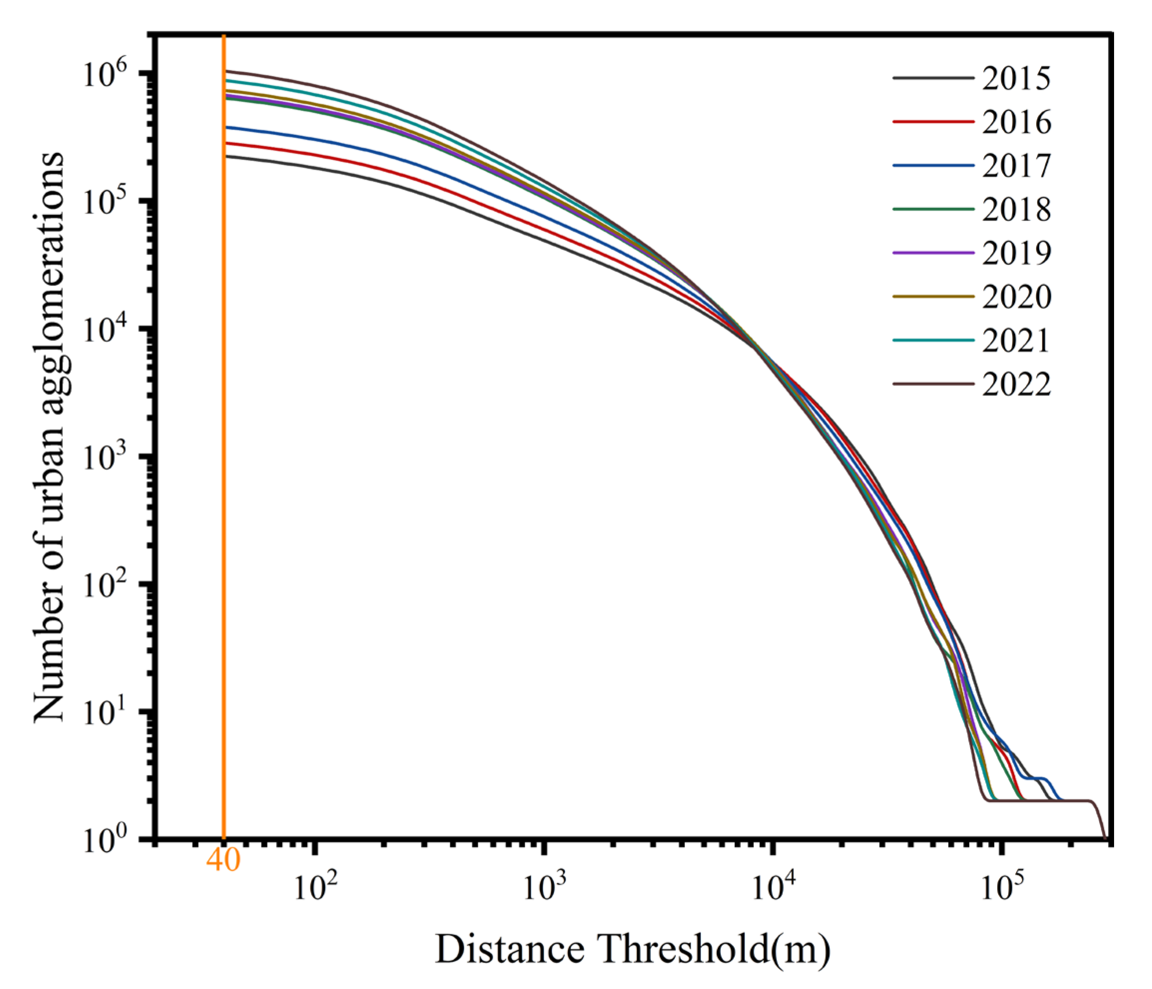
2.2.2. Urban Expansion Curve

Based on the road intersection data, the starting buffer radius is 40 m, and the radius is expanded by 1.1 times until the end. Based on Tannier’s fractal idea, the critical distance threshold corresponding to the extreme value point of curvature on the expansion curve is found to be the buffer radius of road intersections [24], and with the continuous expansion of urban agglomerations, the originally independent urban agglomerations will gradually merge and the number of urban agglomerations will gradually decrease until they become one [41]. Different stages of urban expansion curves represent different stages of urban agglomerations expansion, and a reasonable choice of critical distance thresholds for the corresponding stages is of great significance for portraying the territorial extent of cities. The curvature calculation formula is as follows:

$$\begin{array}{c}K=\frac{y^{″}}{{\left(1+{y^{\prime }}^2\right)}^{\frac{3}{2}}}\end{array}$$

(1)

where K is the curvature of each point of the curve, $y^{″}$ denotes the second-order derivative of the expansion curve, and $y^{\prime }$ denotes the first-order derivative of the expansion curve. By fitting a polynomial to the urban expansion curve, the fitted curve is used to replace the original urban expansion curve. The curvature values are then calculated, and the main curvature points (K) are selected from the extremal points of curvature. The buffering radius corresponding to the main curvature points is the critical distance threshold.

2.2.3. Zipf’s Law

Zipf’s law is described as a special relationship that exists between the size of a city and its corresponding class, a special case where the power-law index is equal to 1 [44]. Zipf’s law, as a tool for studying cities, can be used to study the impact of different factors on urban development at different macro and micro levels. In previous studies, population or economic data are usually used instead of city size, but in reality, there are few cases where the power-law index is strictly equal to 1. Zipf’s law is an ideal state to describe the relationship between city size and its rank. The power-law distribution is represented by the following equation:

$$R_i=A{x}^{-\alpha }$$

(2)

where $R_i$ denotes the city size class, $\alpha$ is a constant, $x$ denotes the city size, and in this paper, the city size is replaced by the area of urban agglomerations, and $\alpha$ is the power-law index. When Zipf’s law is satisfied, the second largest city is one-half the size of the first, the third largest is one-third the size of the first, and so on [45]. The larger the power-law index is, the more balance there is between cities. On the contrary, if the power-law index is less than 1, it means that the agglomerations effect between cities is relatively obvious, and the result is that the larger the large cities, the smaller the small cities. Finding the logarithm for Equation (2) yields the following expressions:

$$\ln (R_i)=\ln A-\alpha \ln x$$

(3)

Equation (3) is fitted using the least squares method, and the power-law index $\alpha$ is calculated. The $\alpha$ values are evaluated for each year, quantifying the development of urban agglomerations. If Zipf’s law is satisfied, the final result obtained is represented on the image as a straight line with slope equal to minus one.

3. Results

3.1. Urban Agglomerations

3.1.1. National-Scale Agglomeration Characteristics

As shown in Figure 3, urban expansion curves were generated for the years 2015 to 2022, and the correlation coefficients were all greater than 0.99 after the polynomial fit. Based on Tannier’s method, the critical distance threshold corresponding to the main curvature point in the urban expansion curve is found to be the buffer radius for generating national urban agglomerations [24].

Table 1. Critical distance thresholds for 2015 to 2022.

Year	Main Curvature Point (K)	Critical Distance Threshold (m)	R2
2015	0.176	121	0.99479
2016	0.333	123	0.99524
2017	0.118	119	0.99598
2018	0.103	117	0.996
2019	0.460	125	0.99441
2020	0.487	126	0.99418
2021	0.645	126	0.99393
2022	0.696	127	0.99376

and Figure 4 present the main curvature points and their corresponding critical distance thresholds from 2015 to 2022, respectively. The curvature extremal points exist within three different stages, where the curvature extremal points of each stage describe different phases of urban development. The first stage (1–100 m) signifies the initial phase of urban expansion, primarily depicting the process of initial integration of urban agglomerations in various central areas. The third stage (1000 m and above) represents the later stage of urban expansion, mainly describing the final phase of agglomerations merging and gradual normalization. However, neither stage represents the main period of urban expansion. Therefore, the curvature extremal points of the second stage (100–1000 m) are selected as the main curvature points [15]. From 2015 to 2022, both the main curvature points and critical distance thresholds increase annually and tend to stabilize.

In China’s urban development process, the construction of urban infrastructure is often faster than the actual population growth. As a result, there are some “Ghost Cities” with no actual population. However, based on the methodology of this paper, these areas are also recognized as urban agglomerations. In fact, the road density in these areas is low, and the distances between urban clusters are far and do not have agglomerations. Considering these reasons, this paper decides to discard this part of the urban agglomerations and only retains the urban agglomerations with an area greater than or equal to 2 buffer zones. A critical distance threshold was used as a buffer radius to generate nationwide urban agglomerations from 2015 to 2022 (Figure 5). Between 2015 and 2022, the number of urban agglomerations increases dramatically nationwide, with discrete, smaller urban agglomerations in distant suburbs integrated into the core areas of urban development and urban agglomerations growing in size [46,47]. On a national scale, the northern and eastern regions are dominated by plains and have a denser road network, which makes it easier for urban agglomerations to integrate, and urban agglomerations are more agglomerative; the southern and western regions are restricted by hills and mountains and have a less dense road network, which makes it less easy for urban agglomerations to integrate with each other, and urban agglomerations are less agglomerative.

The 13th Five-Year Plan proposes to accelerate the development of small and medium-sized cities [6], and from 2015 to 2022, the number of urban agglomerations will grow from 127,284 to 593,301, and the area of urban agglomerations nationwide will grow from 19,673.72 km² to 109,259.38 km². The growth rate of the number of urban agglomerations and the growth rate of the area show a simultaneous increase or decrease. As depicted in Figure 6A, the growth rate of the number of urban agglomerations and the growth rate of the area of urban agglomerations in the country increased sharply for each year, respectively, compared to 2015, and from 2018 onward, the gap between the two became wider, with the growth rate of the area of urban agglomerations being much higher than the growth rate of the number of urban agglomerations. Each year separately shows ups and downs in the number and area of urban agglomerations compared to the previous year until 2020 and a gradual slowdown in the development of urban agglomerations between 2020 and 2022, a period mainly affected by the epidemic, when economic development was severely hampered and urban construction began to slow down. It shows that as cities expand, more and more small and medium-sized urban agglomerations merge to form large urban agglomerations [42], reflecting the strengthening of agglomerations among urban agglomerations. In addition, with the increasing agglomeration effect of large cities, a significant influx of population into cities, continuous optimization of urban infrastructure, and the development and utilization of more suburban land, the growth rate of the urban agglomeration area has surpassed the growth rate of the number of urban agglomerations.

3.1.2. Regional-Scale Aggregation Characteristics

The geographical distribution of urban agglomerations is mainly in the Beijing–Tianjin–Hebei region, the Yangtze River Delta region, the Pearl River Delta region and the Chengdu–Chongqing region (

Table 2. Top five urban agglomerations by area, 2015–2022.

Year	Area (km2)	Cities	Year	Area (km2)	Cities
2015	211.23	Beijing	2019	399.02	Hong Kong, Shenzhen
	75.32	Shenzhen		305.08	Beijing
	70.00	Shanghai		216.90	Chengdu
	68.43	Shenzhen		167.78	Guangzhou
	64.49	Hong Kong		137.92	Shanghai
2016	226.64	Beijing	2020	409.44	Hong Kong, Shenzhen
	97.92	Guangzhou		344.07	Beijing
	92.68	Shenzhen		241.59	Chengdu
	80.73	Shenzhen		174.48	Guangzhou
	77.64	Shanghai		144.13	Shanghai
2017	223.18	Beijing	2021	450.41	Hong Kong, Shenzhen
	198.6	Shenzhen		411.53	Beijing
	106.96	Guangzhou		253.02	Chengdu
	80.01	Shanghai		190.58	Guangzhou
	72.49	Hong Kong		153.13	Shanghai
2018	348.27	Hong Kong, Shenzhen	2022	639.32	Beijing
	267.66	Beijing		602.97	Hong Kong, Shenzhen
	168.13	Chengdu		272.78	Chengdu
	136.35	Guangzhou		248.95	Suqian
	115.77	Shanghai		206.07	Guangzhou

) (Figure 5). The number of urban agglomerations in the Beijing–Tianjin–Hebei region increased from 8.10% in 2015 to 12.00% in 2018 and then decreased to 10.11% in 2022, with the number of urban agglomerations showing a trend of first growth and then decrease. The proportion of the number of urban agglomerations in the Yangtze River Delta region decreased from 25.71% in 2015 to 18.13% in 2022, and the proportion of the number of urban agglomerations showed a decreasing trend year by year. The number of urban agglomerations in the Pearl River Delta region decreased from 9.75% in 2015 to 6.19% in 2022, and the number of urban agglomerations also showed a decreasing trend year by year. The number of urban agglomerations in the Chengdu–Chongqing region grew from 4.62% in 2015 to 6.93% in 2022, and the number of urban agglomerations showed an increasing trend year by year.

The gradual decrease in the number of urban agglomerations as a percentage of the country indicates that different urban agglomerations are gradually merging to form larger urban agglomerations. This phenomenon mainly occurs in the Yangtze River Delta region and the Pearl River Delta region (Figure 7). The Yangtze River Delta region and the Pearl River Delta region are the regions where urban agglomerations were built earlier in China. With the continuous expansion of cities, different urban agglomerations are gradually integrated, resulting in a higher number of urban agglomerations from 2015 to 2017 and a lower number from 2017 to 2022. The Beijing–Tianjin–Hebei region and Chengdu–Chongqing region are relatively economically backward and have late development of urban agglomerations, resulting in a low percentage of urban agglomerations from 2015 to 2017 and a high percentage from 2018 to 2022. The numbers of urban agglomerations in the Beijing–Tianjin–Hebei region and the Chengdu–Chongqing region also start to decrease as a percentage from 2018 and 2022, respectively, indicating that urban agglomerations in the Beijing–Tianjin–Hebei region and the Chengdu–Chongqing region are gradually integrating as cities continue to expand.

The growth of urban agglomerations in China shows four regional distributions, and the five urban agglomerations with the largest areas are extracted for comparative analysis (Table 2), which can explore the reasons for the unevenness of development between different regions. In 2015, the largest difference in the area of the top five urban agglomerations was 146.74 km²; in 2022, the maximum difference grew to 433.25 km², which fully illustrates that as the urban agglomeration area continues to grow, the gap between the urban development of different regions is also increasing. In 2017, Shenzhen’s two separate urban agglomerations merged into one larger urban agglomeration; in 2018, the two larger urban agglomerations of Shenzhen and Hong Kong merged into one mega-urban agglomeration; in 2022, the scattered urban agglomerations of Suqian merged into one large urban agglomeration. These suggest that as cities continue to expand, discrete, smaller urban agglomerations located in suburban areas will eventually merge into existing clustered, larger urban agglomerations.

The main expansion areas of urban agglomerations in China are located in the Beijing–Tianjin–Hebei region, the Yangtze River Delta region, the Pearl River Delta region, and the Chengdu–Chongqing region (Table 2). The top five urban agglomerations in terms of area are all located in the four regions mentioned above. Beijing and Shenzhen have the highest number of occurrences between 2015 and 2022, at eight; this is followed by Guangzhou, Shanghai, and Hong Kong with seven occurrences; Chengdu and Suqian have the least number of occurrences with five and one, respectively. In the Beijing–Tianjin–Hebei region, Beijing is located on the North China Plain, with a dense road network and strong urban agglomerations; in the Yangtze River Delta region, Shanghai has the Huangpu River running through it, and the mega-urban agglomeration is divided into two independent, medium-sized urban agglomerations; Guangzhou, Hong Kong, and Shenzhen are located in the Pearl River Delta region, with urban agglomerations showing multicore expansion and strong intercity agglomerations [48]; Chengdu is located in the plain region, with high road network density and strong urban agglomerations. The development of road networks can reflect the expansion rate of cities from the side [49]. However, the rate of integration of urban agglomerations varies from region to region due to topographic influences.

3.2. Power-Law Index

There is a strong degree of mismatch between the spatial development of urban agglomerations and the administrative setting [22]. Compared with the administrative setting, using urban agglomerations to calculate the power-law index has less error and can quantitatively measure the unevenness of regional development.

Zipf’s law is a special case where the power-law index is equal to 1. However, not all urban agglomerations have a size distribution that exactly satisfies Zipf’s law. Therefore, it is necessary to evaluate the fitting effect of the estimated power-law index and calculate the confidence interval (

Table 3. Presents the power-law indices and their confidence intervals (at a 95% significance level) for the entire country and four regions.

Year	Beijing–Tianjin–Hebei	Yangtze River Delta	Pearl River Delta	Chengdu–Chongqing Region	Nationwide
2015	1.4780	1.4923	1.3078	1.4859	1.4934
	[1.4753,1.4807]	[1.4912,1.4933]	[1.3065,1.3092]	[1.4833,1.4886]	[1.4929,1.4940]
2016	1.4609	1.4612	1.2899	1.4728	1.4759
	[1.4586,1.4632]	[1.4604,1.4620]	[1.2888,1.2911]	[1.4699,1.4757]	[1.4754,1.4763]
2017	1.4499	1.5124	1.3073	1.4334	1.5005
	[1.4478,1.4520]	[1.5115,1.5133]	[1.3063,1.3083]	[1.4316,1.4351]	[1.5001,1.5009]
2018	1.3449	1.4810	1.2889	1.5308	1.4579
	[1.3433,1.3465]	[1.4801,1.4817]	[1.2882,1.2897]	[1.5295,1.5322]	[1.4576,1.4582]
2019	1.2606	1.4107	1.2425	1.4451	1.3917
	[1.2590,1.2622]	[1.4101,1.4113]	[1.2417,1.2433]	[1.4438,1.4465]	[1.3914,1.3920]
2020	1.2413	1.3842	1.2362	1.4416	1.3775
	[1.2398,1.2428]	[1.3836,1.3848]	[1.2354,1.2369]	[1.4404,1.4428]	[1.3772,1.3778]
2021	1.2302	1.3658	1.2520	1.4322	1.3718
	[1.2289,1.2316]	[1.3653,1.3664]	[1.2512,1.2528]	[1.4311,1.4333]	[1.3715,1.3721]
2022	1.2239	1.3407	1.2441	1.4181	1.3583
	[1.2223,1.2251]	[1.3402,1.3412]	[1.2433,1.2449]	[1.4171,1.4191]	[1.3580,1.3586]

). Benguigui proposed a subdimensional standard error, δ, as a criterion, and when δ is less than 0.04, the result is considered acceptable [50], but this method also has limitations. Chen proposed to correct the error by multiplying δ by the threshold of the T-statistic [51], and the confidence interval is calculated as follows:

$${\alpha }^{\ast }=\alpha \left(1\pm \sqrt{\frac{\frac{1}{R^2}-1}{n-2} }{T}_{\tau ,n-2}\right)$$

(4)

where ${\alpha }^{\ast }$ is the upper and lower bounds of the power-law index, $\alpha$ is the estimated power-law index, R² is the correlation coefficient, $\tau$ is the significance level, which is 0.05 in this paper, $n$ is the number of samples used for the estimation, $n-2$ denotes the degrees of freedom, and $T_{\tau ,n-2}$ denotes the statistical threshold.

The size of urban agglomerations in China conforms to a power-law distribution (Figure 8), with a general trend of decreasing year by year, first fast and then slow, except for a slight upward movement in 2017 (Figure 9). The power-law index decreases from 1.49 to 1.36 from 2015 to 2022, showing that the agglomeration of urban agglomerations in China strengthens, and regional unevenness shows a trend of widening.

The Chinese government proposed in 2016 to increase its efforts to develop small and medium-sized cities [6]. As a result, in 2017, the development of small and medium-sized cities strengthened, thus increasing the size of suburban or smallish cities, which made the gap between cities somewhat more even, leading to a high power-law index. While the decreasing power-law index indicates more agglomerations among cities, Beijing, Shanghai, Hong Kong, Guangzhou, and Shenzhen all belong to first-tier cities with earlier urban agglomeration development, while Chengdu belongs to the second-tier cities and Suqian belongs to the third-tier cities, with urban agglomeration area sizes only starting to enter the top five in 2018 and 2022, respectively. As a result, the development of small cities tends to lag behind that of large cities, and the gap between different urban agglomerations will further increase [40].

Chinese urban agglomerations are mainly distributed in the Beijing–Tianjin–Hebei region, Yangtze River Delta region, Pearl River Delta region, and Chengdu–Chongqing region; the above four regions play an important role in the development of Chinese cities, and based on this, this paper extracts the urban agglomerations of the above four regions to calculate the power-law index (Figure 9), and the results are as follows: the power-law indices of all four urban agglomerations show a decreasing trend, with the Beijing–Tianjin–Hebei region showing the largest decreasing trend from 1.48 in 2015 to 1.22 in 2022; the Yangtze River Delta region shows the next largest decreasing trend in the power-law index from 1.49 in 2015 to 1.34 in 2022; the Pearl River Delta region and Chengdu–Chongqing region have the flattest declines in the power-law index, with the Pearl River Delta region power-law index decreasing from 1.31 in 2015 to 1.24 in 2022 and the Chengdu-Chongqing region power-law index decreasing from 1.49 in 2015 to 1.42 in 2022. Among the four regions, the power-law indices of the urban agglomerations are smaller in the Beijing–Tianjin–Hebei region and the Pearl River Delta region, indicating that urban agglomerations are stronger in these two regions. In contrast, the power-law indices of urban agglomerations in the Yangtze River Delta region and the Chengdu–Chongqing region are larger, indicating that the larger urban agglomerations in these two regions are not sufficient to act as agglomerations. The Beijing–Tianjin–Hebei region is located on the North China Plain, with a more developed economy and sparsely distributed water systems, so that discrete, smaller urban agglomerations can easily merge into large urban agglomerations, with stronger urban agglomerations and a lower power-law index. The topography of the Yangtze River Delta region is flat and economically developed, and the gap between small urban agglomerations and large urban agglomerations is small. Urban agglomerations such as Shanghai, Nanjing, and Hangzhou are constrained by the water system, and the urban agglomerations cannot be fully integrated, making the urban agglomerations relatively average in size with a high power-law index. The Pearl River Delta region hosts large urban agglomerations, forming a strong concentration of urban areas. These agglomerations possess favorable conditions for integration and the formation of mega-urban agglomerations, resulting in a lower power-law index. In contrast, the Chengdu–Chongqing region is situated in the interior of the Sichuan basin, with cities scattered far apart. As a result, urban agglomerations in this region face challenges in integration and the formation of mega-urban agglomerations, leading to the highest power-law index.

4. Discussion

The territorial extent of a city is a fundamental property of a city [20], and the discussion of Zipf’s law presupposes the extraction of the territorial extent of a city. Ma and Long start from the community scale and use community data to construct a nationwide urban physical territory [17], but little community-scale administrative division data and population data can be found, and the study has low reproducibility. In addition, many scholars used the combination of remote sensing images and night-light data to identify the territorial extent of cities [31,36,52], but the accuracy of medium- and low-resolution remote sensing images is low, and the overflow of night-light data is strong, which results in large errors [53]. Based on this, the advantages of this study are, first, the low difficulty in obtaining data by using road intersection data to generate nationwide urban clusters; second, compared with the population size, the area of urban agglomerations better reflects the real urban development [39,40,54]; finally, the bottom-up generation of urban agglomerations is not restricted by administrative divisions.

The accuracy of urban territorial extent extracted based on the fractal idea is high in comparison with the results of this paper using the GAIA data mapped by Gong et al. [18]. GAIA data are based on remote sensing images to identify urban impervious surfaces, which are highly dependent on remote sensing image quality and method models and are less effective in identifying discrete urban agglomerations in areas far from urban space (Figure 10). The results of this paper show good identification for both urban areas and areas far from urban space. The suburbs of Beijing, Guangzhou, and Chongqing are all located in mountainous and hilly areas (Figure 10a,b,e–h), which are restricted by topography, and urban agglomerations show a discrete distribution with poor GAIA recognition; recognition is also poorer in areas where land and water meet in the city of Shanghai (Figure 10c,d), and more urban agglomerations are not identified.

Cities themselves are self-similar, and their sizes and outcomes follow many laws [7], with a macro-decentralized and micro-concentrated urban structure having greater development potential [55]. Therefore, the characteristics of cities in different directions, both macro and micro, can be mined on the basis of these laws. Using the population data of Chinese prefecture-level cities from 1990 to 2011, Miao summarized the characteristics of China’s city sizes and finds that the city size of Chinese prefecture-level cities does not satisfy Zipf’s law [30]. Influenced by the household registration system, China has many divisions based on household registration and floating population, and there are large-scale population movements in different cities. Power-law indices calculated using different demographic indicators are significantly different [13]. Other scholars have used multiple sources of data to calculate power-law indices within city administrative divisions [13], but this method still has a large impact on the results because of the connectedness between different cities that develop across administrative boundaries [22]. Gibson et al. mention that using different population divisions to calculate GDP per capita will exacerbate interprovincial inequality and that using different methods to delineate urban areas and calculate population numbers risks overestimating both urban land area and the population within that area [38]. In addition, with China’s rapid economic development, economic, and demographic indicators change frequently, but such changes are not usually easy to detect [37]. For these reasons, the limitations of using population or economic indicators to quantify urban development are clear [40,56]. Using population and GDP data to calculate the power-law index (Figure 11), it can be clearly observed that the power-law index calculated by population size has a large error, and only when the top 100 cities are extracted does the power-law index get a better fit [30], with a power-law index of 2.342. When extended to all cities, the power law fits poorly, with a power-law index of 0.630, which is a difference of more than 270%, and it is much more than the power-law index calculated based on the area of urban clusters, which indicates that assessing the unevenness of urban development from the size of urban population produces a relatively large error.

Cities are complex systems that operate from the bottom up, and the road network, as an internal structure of cities, also exhibits fractal characteristics [57]. Population distribution typically revolves around the road network, and the resulting agglomerations are also shaped by the road network [58]. Numerous smaller urban agglomerations merge to form larger ones, and the area and population density of urban agglomerations decrease as they move away from the road network. Compared to the limitations of population data, the irregular and self-similar fractal features of the road network are closely related to urban characteristics, making the analysis of urban agglomeration changes based on the road network more aligned with the essence of urban evolution. Therefore, exploring the spatiotemporal evolution and differentiation characteristics of the road network can also describe the process of urban expansion and reveal the patterns of urban morphological evolution [28].

Figure 12 shows the relationship between the GDP of prefecture-level cities in China in 2020 and the seventh national census data and the cluster area in the corresponding city administrative area extracted in this paper [59,60]. It can be observed that the urban agglomeration area extracted based on fractal principles exhibits a strong correlation with population and economic scale, with Pearson indices of 0.81 and 0.72, respectively. This indicates that the urban agglomerations generated using road intersections have a significant correlation with population and GDP (Figure 12). However, the correlation between agglomeration area and GDP is relatively weak, indicating that the extracted urban agglomerations can be utilized to quantify the development of cities instead of physical urban areas. Due to the population and economic scale not necessarily developing in tandem with the expansion of the physical urban areas, the speed of urban built-up area expansion is actually faster than the growth rates of the population and economy.

To validate the study’s findings, the GUB data established by Li et al. [20] based on GAIA data were extracted in this paper (Figure 13). The urban agglomerations power-law index is calculated for the whole country and the four regions based on the 2018 GUB data. Nationally, the power-law index is 0.86, indicating that China’s cities do not conform to Zipf’s law at this stage. Among the four regions, the power-law index of the Beijing–Tianjin–Hebei region is 0.97, the power-law index of the Yangtze River Delta and Pearl River Delta regions is 0.80, and the power-law index of the Chengdu–Chongqing region is 0.75. Except for the Beijing–Tianjin–Hebei region, the remaining regions also do not conform to Zipf’s law. The results obtained from the GUB data indicate that cities are more clustered, with larger disparities between different urban agglomerations. First, GUB data identifies the geographical area of the city based on GAIA data. In the urban periphery, GUB data include a large number of non-urban parcels, and the addition of these parcels will make the whole city area larger [15]. Second, in the Pearl River Delta region, the GUB data ignore the influence of topography and identify multiple cities as one urban agglomeration, merging otherwise discrete urban agglomerations (Figure 13e,f). Finally, the GUB data integrate the non-impervious areas within the urban agglomerations and exclude the non-impervious areas far from the urban territory [20], increasing the size of large urban agglomerations and decreasing the size of small and medium-sized urban agglomerations, leading to an increase in the urban agglomerations size gap, which eventually leads to a power-law index of less than 1 and an abnormal power-law index difference in different regions. The results of this paper show that the power-law index difference is smaller and the gap between different regions is more realistic. Compared with the officially delineated cities, the urban agglomerations generated by the urban expansion curve method through the fractal idea are more natural [8,22,61].

From 2015 to 2022, the power-law indices of China’s urban agglomerations all show a decreasing trend, and China’s urban agglomerations gradually conform to Zipf’s law, and the gap between large cities and small cities will further widen. First, due to the unevenness of economic development across regions, large cities have more opportunities and attract more people [48]. Second, due to topographic constraints, urban agglomerations are not easily integrated, and the number of medium and small urban agglomerations increases, resulting in a power-law index greater than 1. In addition, there are more administrative levels, and urban agglomerations are identified by the critical distance threshold set by the urban expansion curve in the geographic space from the provincial, city, and county levels to the township level, increasing the number of small urban agglomerations and making the city size more average in general, pulling up the power-law index. With the end of the COVID-19 pandemic, urban development will gradually accelerate and the urban agglomeration power-law index will decline more rapidly [48]. The decreasing power-law index also further indicates the increasing unevenness of geographical development in China.

There are also shortcomings in this study. The accuracy of the obtained critical distance threshold and urban agglomeration results based on OSM data depends on the precision of the OSM data. However, data timeliness is poorer in urban fringe areas [15]. Furthermore, on the northern plains of China, rural settlements exhibit strong agglomeration tendencies and often integrate with adjacent large urban agglomerations, reflecting greater subjective dependence on urban agglomeration choices away from urban areas. In this paper, we quantify urban development only through the change in the power-law index, but in fact, heavy-tailed graphs such as power-law, lognormal distribution, or exponential function can be used to quantify urban development [62]. Meanwhile, the patterns of urban expansion and population mobility are also potential factors contributing to the decrease in the power-law index. We will subsequently study the changes in Chinese urban agglomerations on longer time series, combining remote sensing imagery and utilizing a variety of statistical ideas, and continue to focus on the relationship between critical distance thresholds, urban power-law distributions, and urban structure. Taking into consideration the influences of different scale ranges, road hierarchy, and other factors, the critical distance threshold is determined to explore the variations in the fractal dimension and power-law index of cities across different scales, ranging from local urban areas to the entire urban region. This study aims to transcend the application of micro-level urban planning and delve into a broader perspective.

5. Conclusions

Overall, the critical distance threshold is closely related to the urban road network. Exploring the evolutionary patterns of the critical distance threshold and power-law index is beneficial for optimizing existing urban structures. Therefore, in this paper, we use the urban expansion curve method to identify the critical distance thresholds from 2015 to 2022 to construct the urban agglomerations in the country from the national scale. This method does not favor cities of scale and retains all urban agglomerations in a more objective way, which can be concluded as follows:

(1)

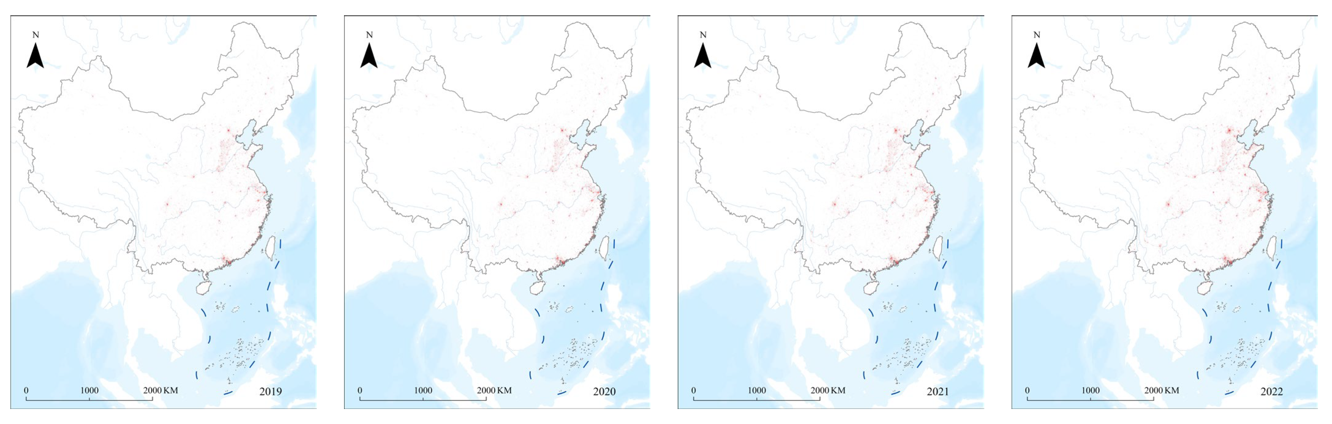
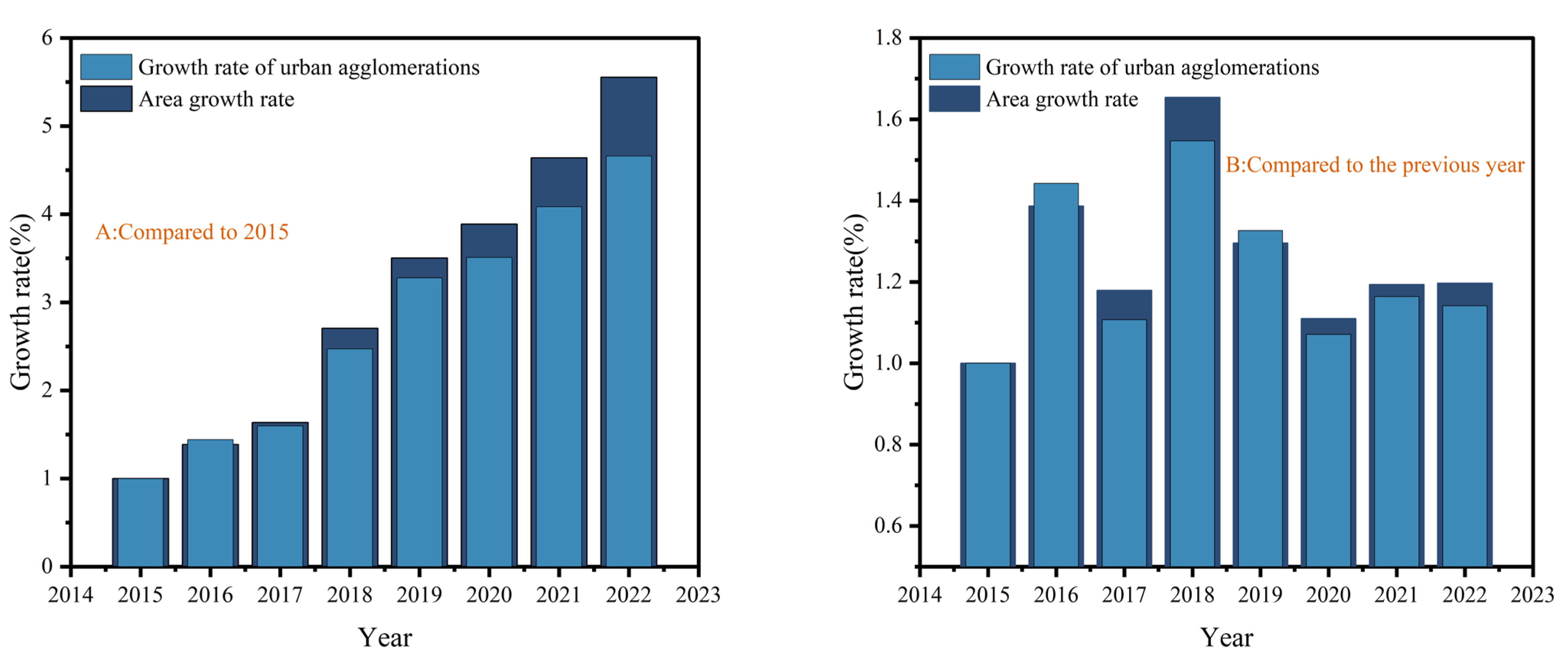
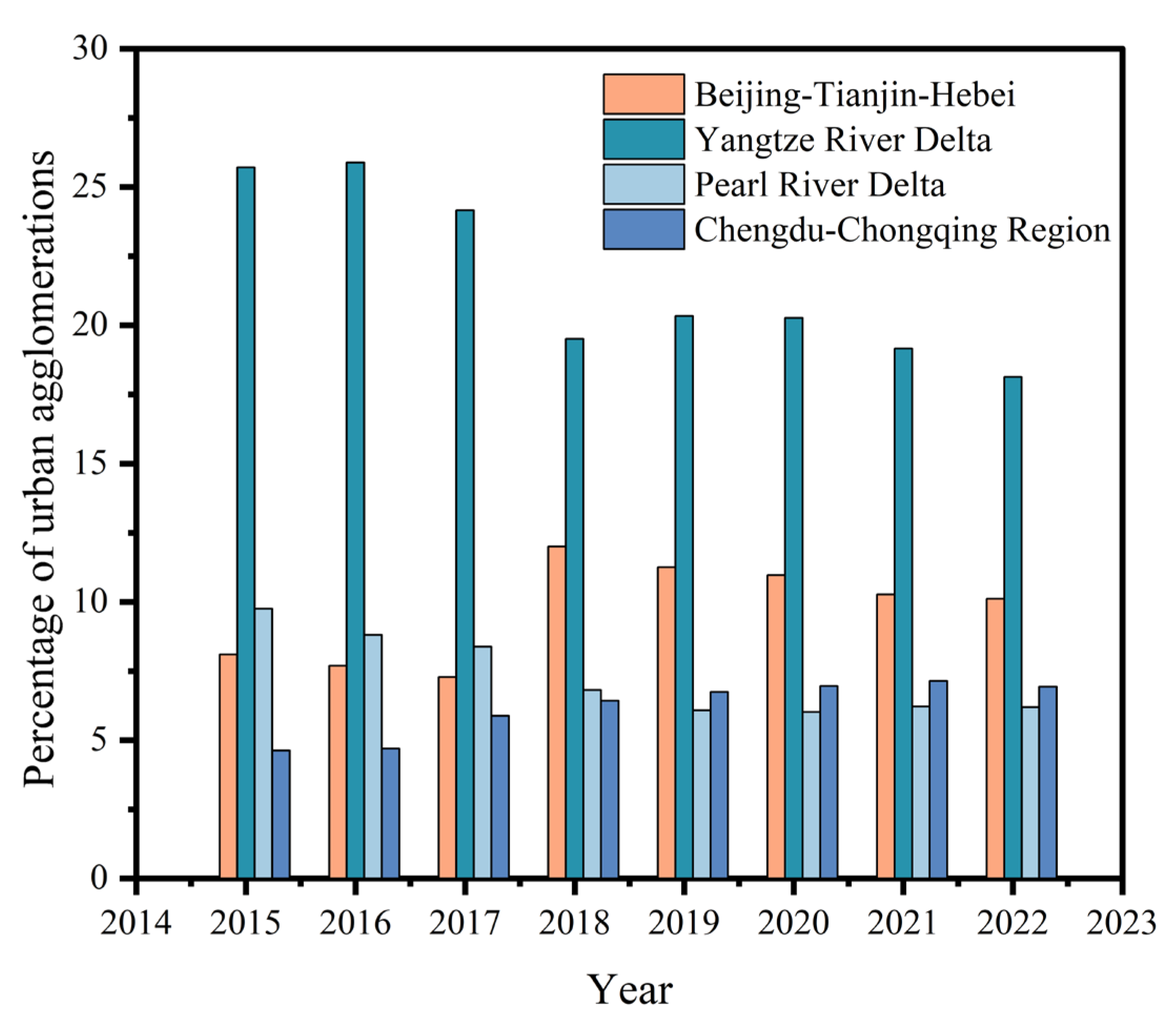
From 2015 to 2022, the growth rate of the number of urban agglomerations and the growth rate of the area in China show a simultaneous growth or decrease. The regions with the most significant growth of urban agglomerations in China are the Beijing–Tianjin–Hebei region, Yangtze River Delta region, Pearl River Delta region, and Chengdu–Chongqing region. The number of agglomerations in the Yangtze River Delta and Pearl River Delta regions decreases year by year, while the number of urban agglomerations in the Beijing–Tianjin–Hebei and Chengdu–Chongqing regions increases year by year. The regions with earlier urban development have a high proportion of urban agglomerations in the early stage and a low proportion in the later stage.

(2)

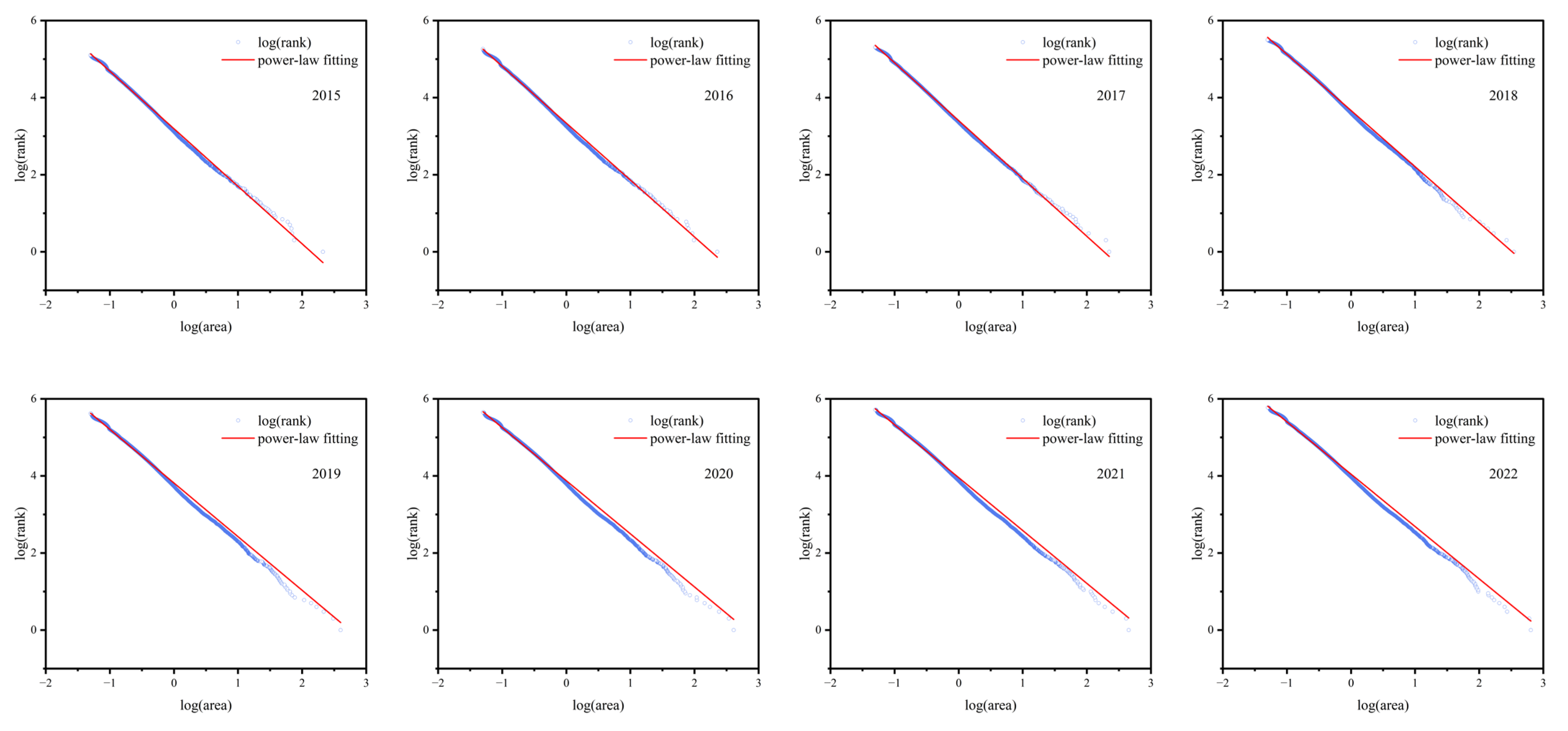
China’s urban agglomerations conform to the power-law distribution law and do not conform to Zipf’s law. From 2015 to 2022, the power-law index of national urban agglomerations decreases year by year, the agglomerations between cities increase, and the unevenness of regional development increases.

(3)

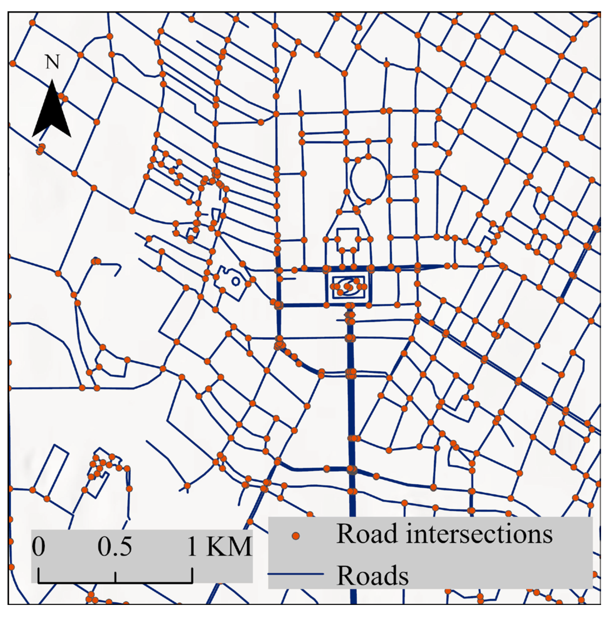
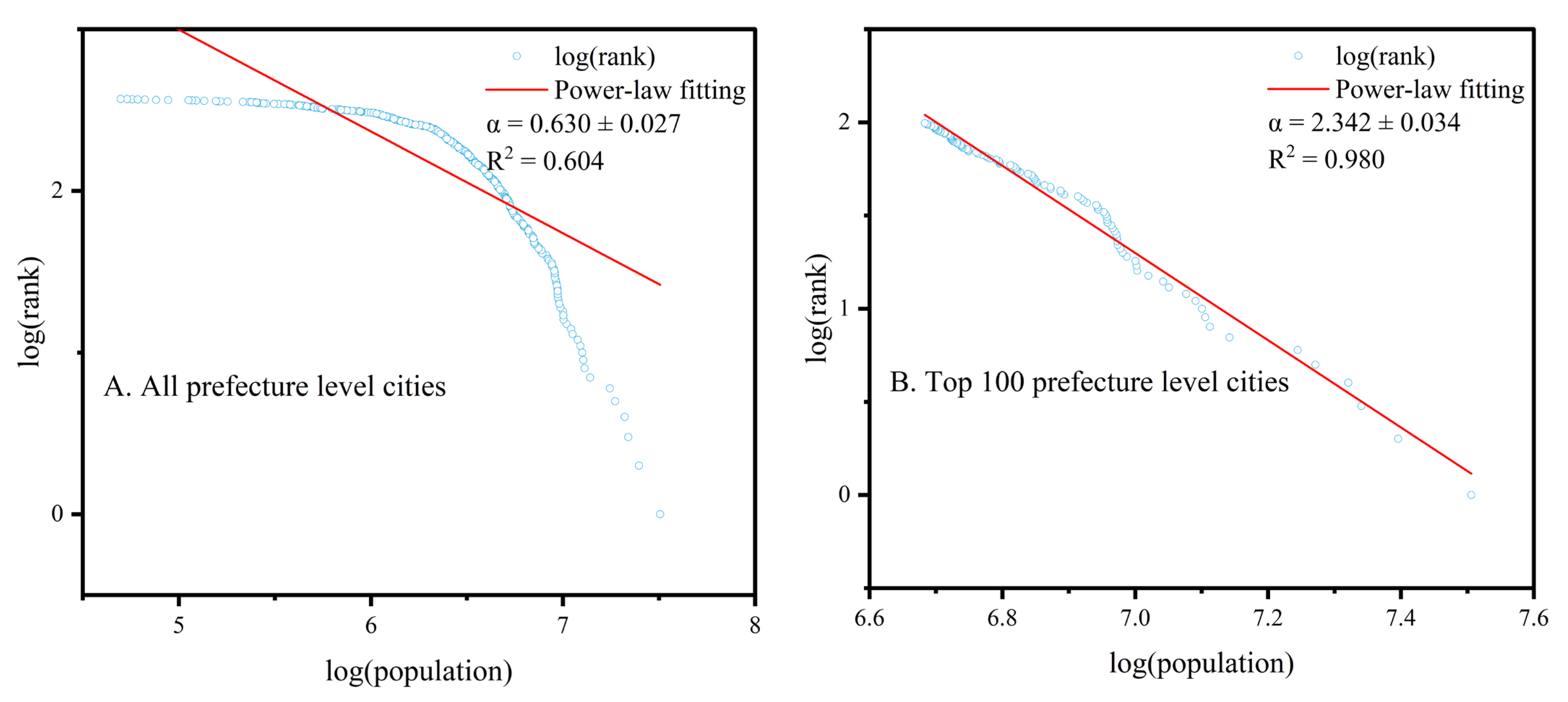
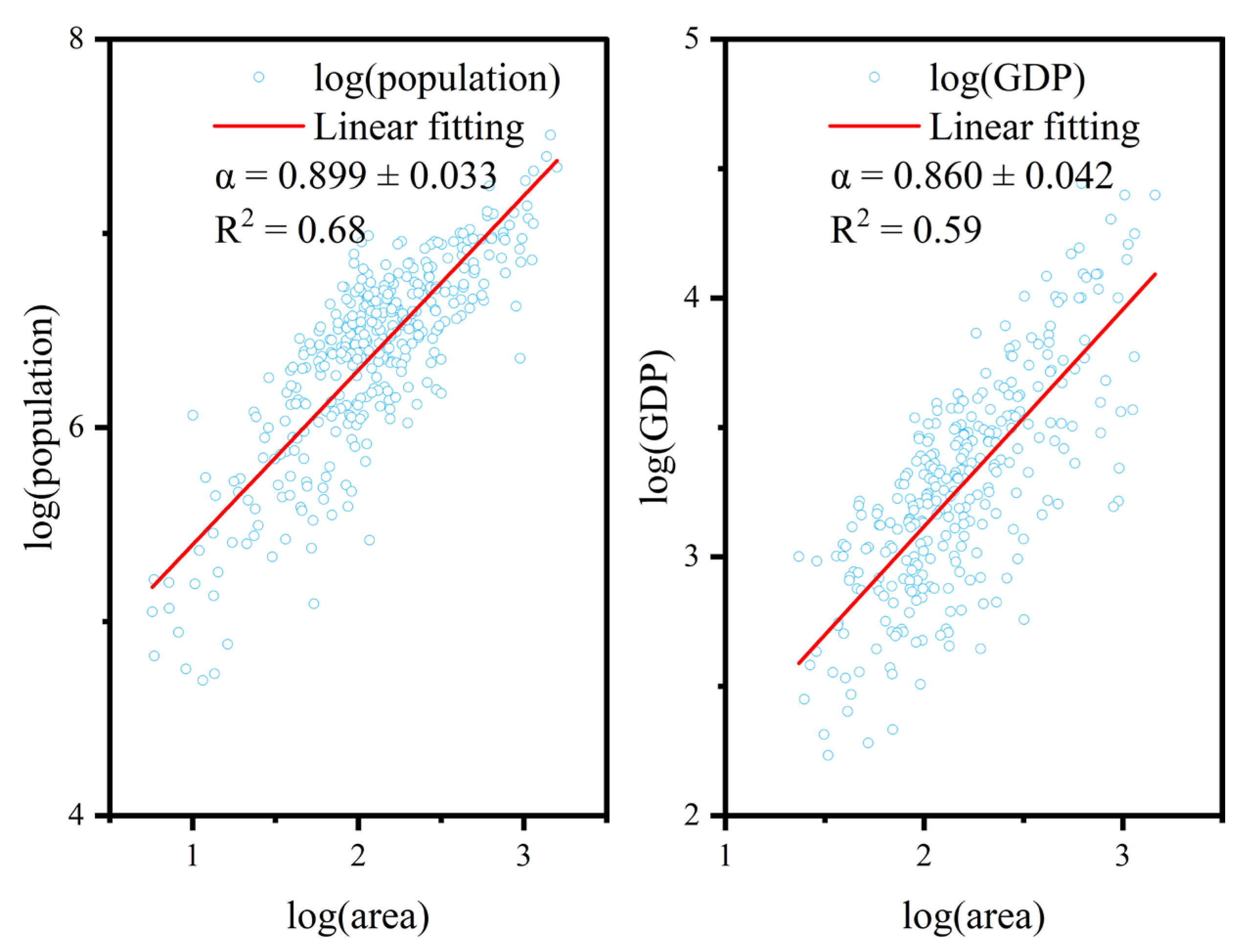
There is a significant correlation between the road network and population data. Chinese urban agglomerations extracted based on road intersections exhibit a linear relationship with officially published population and economic data, indicating that urban agglomerations are expanding faster than the population and economic growth rates.

References

1. Liu, Y.; Li, Y. Revitalize the world’s countryside. Nature 2017, 548, 275–277. [Google Scholar] [CrossRef]
2. Zhong, S.; Wang, M.; Zhu, Y.; Chen, Z.; Huang, X. Urban expansion and the urban–rural income gap: Empirical evidence from China. Cities 2022, 129, 103831. [Google Scholar] [CrossRef]
3. Zhang, X.; Pan, M. Emerging rural spatial restructuring regimes in China: A tale of three transitional villages in the urban fringe. J. Rural Stud. 2022, 93, 287–300. [Google Scholar] [CrossRef]
4. Qu, L.; Li, Y.; Feng, W. Spatial-temporal differentiation of ecologically-sustainable land across selected settlements in China: An urban-rural perspective. Ecol. Indic. 2020, 112, 105783. [Google Scholar] [CrossRef]
5. Li, L.; Ma, S.; Zheng, Y.; Xiao, X. Integrated regional development: Comparison of urban agglomeration policies in China. Land Use Policy 2022, 114, 105939. [Google Scholar] [CrossRef]
6. The Central People’s Government of the People’s Republic of China. Outline of the 13th Five Year Plan for National Economic and Social Development of the People’s Republic of China. Available online: http://www.gov.cn/xinwen/2016-03/17/content_5054992.htm (accessed on 8 April 2023).
7. Batty, M. The Size, Scale, and Shape of Cities. Science 2008, 319, 769–771. [Google Scholar] [CrossRef]
8. Jiang, B.; Jia, T. Zipf’s Law for All the Natural Cities in the United States: A Geospatial Perspective. Int. J. Geogr. Inf. Sci. 2010, 25, 1269–1281. [Google Scholar] [CrossRef]
9. Mori, T.; Smith, T.E.; Hsu, W.-T. Common power laws for cities and spatial fractal structures. Proc. Natl. Acad. Sci. USA 2020, 117, 6469–6475. [Google Scholar] [CrossRef]
10. Zhang, W.; Ma, Y.; Zhu, D.; Dong, L.; Liu, Y. Metrogan: Simulating urban morphology with generative adversarial network. In Proceedings of the 28th ACM SIGKDD Conference on Knowledge Discovery and Data Mining, Washington, DC, USA, 14–18 August 2022; pp. 2482–2492. [Google Scholar]
11. Overman, H.G.; Ioannides, Y.M. Cross-sectional evolution of the US city size distribution. J. Urban Econ. 2001, 49, 543–566. [Google Scholar] [CrossRef]
12. González-Val, R. The evolution of US city size distribution from a long-term perspective (1900–2000). J. Reg. Sci. 2010, 50, 952–972. [Google Scholar] [CrossRef]
13. Sun, X.; Yuan, O.; Xu, Z.; Yan, h.; Liu, Q.; Wu, L. Did Zipf’s Law hold for Chinese cities and why? Evidence from multisource data. Land Use Policy 2021, 106, 105460. [Google Scholar] [CrossRef]
14. Wang, H.; Ning, X.; Zhang, H.; Liu, Y. Urban Expansion Analysis of China’s Prefecture Level City from 2000 to 2016 using High-Precision Urban Boundary. In Proceedings of the IGARSS 2019—2019 IEEE International Geoscience and Remote Sensing Symposium, Yokohama, Japan, 28 July–2 August 2019; pp. 7514–7517. [Google Scholar]
15. Kong, L.; He, Z.; Chen, Z.; Luo, M.; Du, Z.; Zhu, F.; He, L. Spatial Distribution and Morphological Identification of Regional Urban Settlements Based on Road Intersections. ISPRS Int. J. Geo-Inf. 2021, 10, 4. [Google Scholar] [CrossRef]
16. Zhou, Y.; Shi, Y. Toward establishing the concept of physical urban area in China. Acta Geogr. Sin. 1995, 50, 289–301. [Google Scholar]
17. Ma, S.; Long, Y. Identifying Spatial Cities in China at the Community Scale. J. Urban Reg. Plan. 2019, 11, 37–50. [Google Scholar]
18. Gong, P.; Li, X.; Wang, J.; Bai, Y.; Zhou, Y. Annual maps of global artificial impervious area (GAIA) between 1985 and 2018. Remote Sens. Environ. 2019, 236, 11510. [Google Scholar] [CrossRef]
19. Qin, Y.; Xiao, X.; Dong, J.; Chen, B.; Liu, F.; Zhang, G.; Zhang, Y.; Wang, J.; Wu, X.J.I.J.o.P.; Sensing, R. Quantifying annual changes in built-up area in complex urban-rural landscapes from analyses of PALSAR and Landsat images. ISPRS J. Photogramm. Remote Sens. 2017, 124, 89–105. [Google Scholar] [CrossRef]
20. Li, X.; Gong, P.; Zhou, Y.; Wang, J.; Bai, Y.; Chen, B.; Hu, T.; Xiao, Y.; Xu, B.; Yang, J. Mapping global urban boundaries from the global artificial impervious area (GAIA) data. Environ. Res. Lett. 2020, 15, 094044. [Google Scholar] [CrossRef]
21. Tan, X.; Chen, Y. Urban boundary identification based on neighborhood dilation. Prog. Geogr. 2015, 34, 1259–1265. [Google Scholar]
22. Long, Y. Redefining Chinese city system with emerging new data. Appl. Geogr. 2016, 75, 36–48. [Google Scholar] [CrossRef]
23. Rozenfeld, H.D.; Rybski, D.; Gabaix, X.; Makse, H.A. The Area and Population of Cities: New Insights from a Different Perspective on Cities. Am. Econ. Rev. 2011, 101, 2205–2225. [Google Scholar] [CrossRef]
24. Tannier, C.; Thomas, I.; Vuidel, G.; Frankhauser, P. A fractal approach to identifying urban boundaries. Geogr. Anal. 2011, 43, 211–227. [Google Scholar] [CrossRef]
25. Zhang, H.; Lan, T.; Li, Z. Fractal evolution of urban street networks in form and structure: A case study of Hong Kong. Int. J. Geogr. Inf. Sci. 2022, 36, 1100–1118. [Google Scholar] [CrossRef]
26. Agostinho, F.; Costa, M.; Coscieme, L.; Almeida, C.M.; Giannetti, B.F. Assessing cities growth-degrowth pulsing by emergy and fractals: A methodological proposal. Cities 2021, 113, 103162. [Google Scholar] [CrossRef]
27. Li, D.; Li, X. An Overview on Data Mining of Nighttime Light Remote Sensing. Acta Geod. Cartogr. Sin. 2015, 44, 591–601. [Google Scholar]
28. Chen, S.; Zhang, H.; Ou, X. Study on the spatial-temporal differentiation of road network density and its relationship with urban form in Greater Bay Area of Guangdong, Hong Kong and Macao. In Proceedings of the 3rd International Conference on Internet of Things and Smart City (IoTSC 2023), Chongqing, China, 24–26 March 2023; pp. 310–319. [Google Scholar]
29. He, B.; Guo, R.; Li, M.; Jing, Y.; Zhao, Z.; Zhu, W.; Zhang, C.; Zhang, C.; Ma, D. The fractal or scaling perspective on progressively generated intra-urban clusters from street junctions. Int. J. Digit. Earth 2023, 16, 1944–1961. [Google Scholar] [CrossRef]
30. Miao, H. Analysis of the evolutionary characteristics of city size distribution of prefecture-level cities in China. Inq. Econ. Issues 2014, 113–121. [Google Scholar] [CrossRef]
31. Chen, Z.; Wei, Y.; Shi, K.; Zhao, Z.; Wang, C.; Wu, B.; Qiu, B.; Yu, B. The potential of nighttime light remote sensing data to evaluate the development of digital economy: A case study of China at the city level. Comput. Environ. Urban Syst. 2022, 92, 101749. [Google Scholar] [CrossRef]
32. Chen, Y. Exploring the level of urbanization based on Zipf’s scaling exponent. Phys. A Stat. Mech. Appl. 2020, 566, 125620. [Google Scholar] [CrossRef]
33. Wan, G.; Zhu, D.; Wang, C.; Zhang, X. The size distribution of cities in China: Evolution of urban system and deviations from Zipf’s law. Ecol. Indic. 2020, 111, 106003. [Google Scholar] [CrossRef]
34. Holmes, T.J.; Lee, S. Cities as Six-by-Six-Mile Squares: Zipf’s Law? In Agglomeration Economics; Glaeser, E.L., Ed.; The University of Chicago Press: Chicago, IL, USA, 2010; Volume 3, pp. 105–131. [Google Scholar]
35. Arshad, S.; Hu, S.; Ashraf, B.N. Zipf’s Law, the Coherence of the Urban System and City Size Distribution: Evidence from Pakistan. Phys. A Stat. Mech. Appl. 2019, 513, 87–103. [Google Scholar] [CrossRef]
36. Cao, W.; Dong, L.; Wu, L.; Liu, Y. Quantifying urban areas with multi-source data based on percolation theory. Remote Sens. Environ. 2020, 241, 111730. [Google Scholar] [CrossRef]
37. Holz, C.A.J.S.E.J. Chinese Statistics: Classification Systems and Data Sources. SSRN Electron. J. 2013, 54, 532–571. [Google Scholar]
38. Gibson, J.; Li, C. The erroneous use of china’s population and per capita data: A structured review and critical test. J. Econ. Surv. 2017, 31, 905–922. [Google Scholar] [CrossRef]
39. Nitsch, V. Zipf zipped. J. Urban Econ. 2005, 57, 86–100. [Google Scholar] [CrossRef]
40. Kosmopoulou, G.; Buttry, N.; Johnson, J.; Kallsnick, A. Suburbanization and the rank-size rule. Appl. Econ. Lett. 2007, 14, 1–4. [Google Scholar] [CrossRef]
41. Wang, D.; Kong, L.; Chen, Z.; Yang, X.; Luo, M. Physical Urban Area Identification Based on Geographical Data and Quantitative Attribution of Identification Threshold: A Case Study in Chongqing Municipality, Southwestern China. Land 2023, 12, 30. [Google Scholar] [CrossRef]
42. Hu, T.; Huang, X.; Li, X.; Liang, L.; Xue, F. Toward a better understanding of urban sprawl: Linking spatial metrics and landscape networks dynamics. In Computational Urban Planning and Management for Smart Cities; Springer: Cham, Switzerland, 2019; pp. 163–178. [Google Scholar]
43. National Bureau of Statistics. China Statistical Yearbook. Available online: http://www.stats.gov.cn/sj/ndsj/ (accessed on 8 April 2023).
44. Bettencourt, L.; Zünd, D. Demography and the Emergence of Universal Patterns in Urban Systems. Nat. Commun. 2020, 11, 4584. [Google Scholar] [CrossRef]
45. Eeckhout, J. Gibrat’s Law for (All) Cities. Am. Econ. Rev. 2004, 94, 1429–1451. [Google Scholar] [CrossRef]
46. Dietzel, C.; Herold, M.; Hemphill, J.J.; Clarke, K.C. Spatio-temporal dynamics in California’s Central Valley: Empirical links to urban theory. Int. J. Geogr. Inf. Sci. 2005, 19, 175–195. [Google Scholar] [CrossRef]
47. Bosch, M.; Jaligot, R.; Chenal, J. Spatiotemporal patterns of urbanization in three Swiss urban agglomerations: Insights from landscape metrics, growth modes and fractal analysis. Landsc. Ecol. 2020, 35, 879–891. [Google Scholar] [CrossRef]
48. Yin, C.; Meng, F.; Yang, X.; Yang, F.; Fu, P.; Yao, G.; Chen, R. Spatio-temporal evolution of urban built-up areas and analysis of driving factors—A comparison of typical cities in north and south China. Land Use Policy 2022, 117, 106114. [Google Scholar] [CrossRef]
49. Wei, W.; Shi, P.J.; Zhou, J.J.; Xie, B.B. The Road Network Density and Spatial Dependence Analysis Based on Basin Scale—A Case Study on Shiyang River Basin. Appl. Mech. Mater. 2014, 505–506, 750–754. [Google Scholar] [CrossRef]
50. Benguigui, L.; Czamanski, D.; Marinov, M.; Portugali, Y.J.E. When and where is a city fractal? Environ. Plan. B:Plan. Des. 2000, 27, 507–519. [Google Scholar] [CrossRef]
51. Chen, Y. Approaches to estimating fractal dimension and identifying fractals of urban form. Prog. Geogr. 2017, 36, 529–539. [Google Scholar]
52. Jing, W.; Yang, Y.; Yue, X.; Zhao, X. Mapping Urban Areas with Integration of DMSP/OLS Nighttime Light and MODIS Data Using Machine Learning Techniques. Remote Sens. 2015, 7, 12419–12439. [Google Scholar] [CrossRef]
53. Imhoff, M.L.; Lawrence, W.T.; Elvidge, C.D.; Paul, T.; Levine, E.; Privalsky, M.V.; Brown, V. Using nighttime DMSP/OLS images of city lights to estimate the impact of urban land use on soil resources in the United States. Remote Sens. Environ. 1997, 59, 105–117. [Google Scholar] [CrossRef]
54. Gabaix, X. Zipf’s law for cities: An explanation. Q. J. Econ. 1999, 114, 739–767. [Google Scholar] [CrossRef]
55. Feng, W.; Li, B.; Chen, Z.; Liu, P. City size based scaling of the urban internal nodes layout. PLoS ONE 2021, 16, e0250348. [Google Scholar] [CrossRef]
56. Arcaute, E.; Hatna, E.; Ferguson, P.; Youn, H.; Johansson, A.; Batty, M. Constructing cities, deconstructing scaling laws. J. R. Soc. Interface 2015, 12, 20140745. [Google Scholar] [CrossRef]
57. Sahitya, K.S.; Prasad, C. Urban road network structural analysis and its relation with human settelements using geographical information systems. Suranaree J. Sci. Technol. 2021, 28, 010084. [Google Scholar]
58. Ji, W.; Wang, Y.; Zhuang, D.; Song, D.; Shen, X.; Wang, W.; Li, G. Spatial and temporal distribution of expressway and its relationships to land cover and population: A case study of Beijing, China. Transp. Res. Part D Transp. Environ. 2014, 32, 86–96. [Google Scholar] [CrossRef]
59. National Bureau of Statistics. Major Figures on 2020 Population Census of China. Available online: http://www.stats.gov.cn/sj/pcsj/rkpc/d7c/ (accessed on 9 August 2023).
60. National Bureau of Statistics. China Statistical Yearbook 2020. Available online: http://www.stats.gov.cn/sj/ndsj/2020/indexch.htm (accessed on 9 August 2023).
61. Tannier, C.; Thomas, I. Defining and characterizing urban boundaries: A fractal analysis of theoretical cities and Belgian cities. Comput. Environ. Urban Syst. 2013, 41, 234–248. [Google Scholar] [CrossRef]
62. Wang, J.; Lu, F.; Liu, S. A classification-based multifractal analysis method for identifying urban multifractal structures considering geographic mapping. Comput. Environ. Urban Syst. 2023, 101, 101952. [Google Scholar] [CrossRef]
Figure 1. Experimental procedures.
Ijgi 12 00472 g001
Figure 2. Local road intersections in 2015.
Ijgi 12 00472 g002
Figure 3. Urban expansion curve from 2015 to 2022.
Ijgi 12 00472 g003
Figure 4. The curvature variation of urban expansion curve in China from 2015 to 2022.
Ijgi 12 00472 g004aIjgi 12 00472 g004b
Figure 5. National urban agglomerations distribution map from 2015 to 2022.
Ijgi 12 00472 g005aIjgi 12 00472 g005b
Figure 6. Growth rate of urban agglomerations in number and area: (A) is compared to 2015; (B) is compared to the previous year.
Ijgi 12 00472 g006
Figure 7. Percentage of the number of urban agglomerations in the four regions.
Ijgi 12 00472 g007
Figure 8. A power-law fit to the national urban agglomeration sizes from 2015 to 2022.
Ijgi 12 00472 g008
Figure 9. National and four regional power-law index changes.
Ijgi 12 00472 g009
Figure 10. Comparison with GAIA data: Beijing (a,b), Shanghai (c,d), Guangzhou (e,f), and Chongqing (g,h).
Ijgi 12 00472 g010
Figure 11. Power-law fit based on the seventh census data.
Ijgi 12 00472 g011
Figure 12. Urban agglomerations size in relation to population and GDP.
Ijgi 12 00472 g012
Figure 13. Comparison of GUB data: Beijing (a,b), Shanghai (c,d), Guangzhou (e,f), and Chongqing (g,h).
Ijgi 12 00472 g013