Batch Simplification Algorithm for Trajectories over Road Networks

Abstract

The steady increase in data generation by GPS systems poses storage challenges. Previous studies show the need to address trajectory compression. The demand for accuracy and the magnitude of data require effective compression strategies to reduce storage. It is posited that the combination of TD-TR simplification, Kalman noise reduction, and analysis of road network information will improve the compression ratio and margin of error. The GR algorithm is developed, integrating noise reduction and path compression techniques. Experiments are applied with trajectory data sets collected in the cities of California and Beijing. The GR algorithm outperforms similar algorithms in compression ratio and margin of error, improving storage efficiency by up to 89.090%. The combination of proposed techniques presents an efficient solution for GPS trajectory compression, allowing to improve storage in trajectory analysis applications.

1. Introduction

In the current landscape of the geospatial information age, the steady increase in data generation by global positioning systems (GPS) poses unprecedented challenges in terms of efficient information management and storage. The massive collection of location data, driven by the proliferation of GPS devices and related applications, has led to the creation of vast data sets that require innovative solutions in terms of compression and processing. As mobile devices, vehicles and other systems incorporate location technologies, the amount of data generated grows exponentially, which in turn requires ingenious approaches to reduce the storage footprint without compromising the quality and accuracy of the information.

The GPS trajectory simplification field is still a subject of ongoing research. As location technology evolves and is applied in various domains, challenges arise in efficiently processing geospatial data. Simplifying trajectories becomes more challenging due to increasing complexity, which is caused by factors such as traffic and mobility patterns. Furthermore, agile approaches are required to handle real-time data dynamics. These improvements are crucial for optimizing the handling of geospatial data in various applications, from personalized navigation to urban planning [1]. Therefore, the research on simplification algorithms optimizes not only the volume of data but also enables more efficient pattern extraction, benefiting various disciplines that depend on geospatial information [2]. Nevertheless, the documentary analysis identified common deficiencies in trajectory simplification algorithms. These shortcomings negatively impact the efficacy of simplification algorithms.

Therefore, the following research questions are posed: How to increase the data compression ratio in GPS trajectory preprocessing? How does the incorporation of a noise reduction component influence GPS trajectory simplification? What is the impact of using road network analysis in the GPS trajectory simplification process? These questions will be answered at the end of this study. In this context, the objective of the research is to develop a GPS trajectory simplification algorithm in order to increase the data compression ratio, based on noise reduction, trajectory simplification and road network information.

This paper proposes a GPS vehicle trajectory simplification algorithm that considers noise reduction, point simplification and road network information analysis.

This article is organized as follows: Section 1 contains an introduction where the problem is identified, Section 2 contains related works that were identified in the literature and present different solutions to the problem are analyzed, Section 3 describes the proposed algorithm, Section 4 presents the obtained results, Section 5 discusses the results and finally Section 6 contains the conclusions and lines of future work.

2. Related Work

The volume of generated data by global positioning systems (GPS) around the world is resulting in ever-increasing information storage requirements. Studies [3,4,5,6] have shown that, without compression and at 10-s collection intervals, 100 megabytes (MB) are stored for every 400 objects in a single day. Longer-term studies highlight that if you collect movement data from 10,000 users based on their geographic position every 15 s, you generate more than 50 million data per day and approximately 20 trillion data per year [7,8,9].

Data compression forms a crucial part of the data preparation and analysis phase [10]. Compression algorithms can be classified into two categories, lossless and lossy compression algorithms. Lossless compression algorithms perform a more accurate reconstruction of the original data without loss of information. In contrast, lossy compression algorithms exhibit inaccuracies compared to the original data [11].

The main advantage of lossy compression is that it can drastically reduce storage requirements while maintaining an acceptable degree of error [12,13]. If an acceptable error range can be maintained, lossy compression is effective when dealing with large volumes of data.

A trajectory is represented as a discrete sequence of geographic coordinate points [4]. An example of trajectories are vehicular trajectories that are composed of thousands of points, since the stretches traveled in cities are usually long and with many stops, which implies a greater emission of coordinates generated from GPS devices.

There are currently active research related areas to GPS trajectories [14,15]. Among them is the area of trajectory pre-processing which studies trajectory simplification techniques and algorithms. The trajectory simplification algorithms eliminate some subtraces of the original trajectory [16]; which decreases the data storage space and the data transfer time [17,18,19]. A framework where these areas are observed is proposed in this paper [20].

Reducing the size of the data in a trajectory facilitates the acceleration of the information extraction process [12,21]. There are several path simplification methods and algorithms that are suitable for different types of data and yield different results [22]; but they all have the same principle in common: simplify the data by removing the redundancy of the data in the source file [23,24,25,26]. Meratnia et al. [27] define data compression as substantially reducing the amount of data without significant loss.

As can be seen, both terms have points of contact, so it is considered that in the consulted literature so far, the terms compression and simplification of GPS trajectories are used interchangeably to refer to the elimination of data redundancy. In the present work the term simplification is adopted when it refers to the elimination of redundancy of points of the original trajectory.

GPS trajectory simplification algorithms can be classified into: online algorithms and batch algorithms [28]. Online algorithms do not need to have the entire trajectory ready before starting the simplification, and are suitable for compressing trajectories in mobile device sensors [29,30,31,32]. Online algorithms not only have good compression ratios and deterministic error bounds, but are also easy to implement. They are widely used in practice, even for freely moving objects without the constraint of road networks [29,32,33,34].

Batch algorithms require all points in the trajectory before starting the simplification, which allows them to perform better processing and analysis of these [35]. The advantages of some of the analyzed algorithms [36] are:

• Douglas-Peucker: Performs point simplification accurately in terms of the spatial error metric. By taking a parameter error threshold, it ensures that the error of the simplified trajectory is within the bounds of the target application [37];
• TD-TR: By using the synchronous Euclidean distance for the calculations, this allows you to guarantee both a maximum spatial distance and a maximum temporal error distance;
• Window opening algorithm: Processing time is very low;
• ST-Trace: Uses the velocity and orientation of the trajectory points in the simplification step [38].

The noisy nature of GPS data is an important element to take into account, however, in the consulted literature there are few examples of GPS trajectory simplification algorithms that take this aspect into account. An example of this is proposed by Gomez et al. [39], where a Kalman filter is used to improve the accuracy of low-cost readers. That work shows that the use of a filtering technique, as a prior step, in the GPS trajectory simplification algorithm significantly improves the results of the simplification process. Data filtering is an important preliminary step to take into account and is one of the limitations of the currently proposed algorithms, which do not take into account the level of noise that a trajectory may have.

Two types of noises to which GPS trajectories are exposed and simplification algorithms do not take into account are exposed by Corcoran et al. [4]. The two types are:

• Trajectories may contain outliers;
• The points of a trajectory may have a localization error.

Ivanov [40] presented an online GPS trajectory simplification method, which explicitly states that it does not take into account the presented noise by the trajectory and therefore cannot be used for navigation.

The GPS trajectories obtained from the sensors on vehicles traveling on the road network contain information from this same network expressed in the form of geographic coordinates [41]. Several systems used to represent these trajectories (geographic information systems) contain among their layers the road network information layer. In this way it is possible to represent the trajectories on the map.

The GPS trajectory simplification algorithms proposed in the literature [42,43,44] only eliminate data that are considered redundant in the GPS trajectory in such a way that they do not affect its representation [45]. This process is performed without taking into account the information of the road network through which the traveled vehicle, however, the analysis of this information in the elimination of data resulting from the simplification process could be used to consider the relevance of keeping or eliminating a simplified data [46,47]. This analysis is not performed in the algorithms, described in the literature and there are works that use this information to improve the representation of simplified trajectories with the Douglas-Peucker algorithm [48].

Among the limitations of GPS trajectory simplification algorithms, described in the literature [36,42,49] are:

• Douglas-Peucker: Only performs spatial analysis of the data;
• Visvalingam: The compression ratio is reduced and only performs spatial analysis;
• TD-TR: It presents a smaller margin of error in the trajectory simplification process and an acceptable compression ratio. A limitation is the processing time;
• Lang: Its point elimination method is trivial, so it discards points considered significant, increasing its margin of error;
• Window Aperture: Its main disadvantage is the frequent elimination or misrepresentation of important points such as acute angles. A secondary limitation is that straight lines are still over-represented. It requires high hardware performance for proper operation;
• ST-Trace: Processing time is considerable and requires velocity information to characterize the trace.

From the documentary analysis performed, a set of common deficiencies in the aforementioned trajectory simplification algorithms were identified [50]. These deficiencies that undermine the effectiveness of the simplification algorithms are discussed below:

• None of the analyzed algorithms consider the noise present in the trajectory data, which reduces the possibility of eliminating points that are not significant during the simplification process;
• Only the Squish and Dots algorithms perform a rigorous analysis of the GPS trajectory decoding procedure, but do not consider the analysis of trajectory noise;
• Douglas Peucker, Visvalingam and Window opening only perform spatial analysis of the data. This removes temporal information that provides data of importance to achieve a better compression ratio;
• Visvalingam removes or misrepresents points, such as acute angles, so the resulting trajectory may lack important points for reconstructing a path;
• None of the algorithms consider network information in trajectory simplification, missing the opportunity to perform an analysis that allows more points of little significance to be discarded from the original trajectory.

A comparison of simplification methods proposed for trajectories used by other authors is presented in Table 1.

Table 1. Comparison of simplification methods proposed for trajectories used by other authors.

Article	Hypothesis	Used Method	Compression Behavior
A Trajectory Compression Algorithm Based on Non-uniform Quantization (2015)	Large volume of spatiotemporal trajectory data generates high overhead for data storage, transmission and processing.	An algorithm for trajectory compression based on non-uniform quantization is employed.	Improved compression ratio when processing large-scale trajectory data and in a geographical context.
Improvement of OPW-TR Algorithm for Compressing GPS Trajectory Data (2017)	A compression algorithm can reduce the size of trajectory data and minimize information loss.	An improved algorithm for open window time ratio (OPW-TR).	The errors of the algorithm are smaller than existing algorithms in terms of SED.
A Heading Maintaining Oriented Compression Algorithm for GPS Trajectory Data (2019)	Compression of trajectory data considering heading up to a maximum spatial error achieves more accurate approximation.	A heading-oriented trajectory compression algorithm takes into account position and heading information.	The algorithm can guarantee some effect on heading information and is more flexible.
Simplified Algorithm of Moving Object Trajectory Based on Interval Floating (2022)	Simplified Algorithm of Moving Object Trajectory Based on Interval Floating.	Techniques such as angular deviation, the sum of angular deviations, threshold evaluations.	The algorithm has an improved simplification rate with some simplification error.
AIS Trajectories Simplification Algorithm Considering Topographic Information (2022)	A novel algorithm that simplifies AIS trajectories considering topographic information is proposed.	Improved Douglas-Peucker algorithm using quadtree of random polygon maps.	Simplified trajectories without intersections were produced with superior computational efficiency.

This paper proposes a GPS vehicle trajectory simplification algorithm that considers noise reduction, point simplification and road network information analysis. For this purpose, an area to be processed is selected according to the position of the GPS records within a road network. The area is delimited at the beginning of the process and its size depends on the number of identified outlier points and the zones to which they belong because they will be excluded from the area to be processed. Then, using a batch simplification technique that considers the temporal dimension, each GPS point of the trajectory is processed to reduce the noise present in the trajectory and an analysis is performed with the corresponding road network information to decide whether or not the GPS point is part of the final simplified trajectory. This algorithm can be used, along with other tools, for data compression methods that will allow intelligent transportation systems to improve the processing and storage of these large volumes of data. The proposed algorithm was used to process areas corresponding to GPS trajectories from two public datasets: Geolife and Mobile Century.

3. Materials and Methods

From the literature review, a set of common shortcomings in trajectory simplification algorithms have been identified. One of the main limitations is that these algorithms do not take into account the nature of the data and present compression ratio rates that can be improved. To improve the compression ratio rates, and based on a spatio-temporal batch simplification algorithm, the reduction of noise present in the trajectory and the simplification of points can be included with the analysis of road network information.

In this paper, a new GPS trajectory simplification algorithm called “GR Simplification” is proposed which considers noise reduction, point simplification and road network information analysis.

3.1. Noise Reduction

The main objective of noise reduction is the elimination of outliers by correcting the points of the trajectory from an initial state, as the author of this work demonstrates by Reyes et al. [51]. For this purpose, the Kalman noise reduction logic is applied, which takes into account the characteristics of the problem to be treated. Initially, a model is constructed, closely related to the data of the trajectories to be analyzed in order to adjust the filter. The definition used in this article is supported by Lin et al. [52] because it makes use of the mathematical model for a 4-wheel vehicle.

The modeling of the motion problem for the Kalman filter logic is defined in this paper by the equations of motion (Equations (1) and (2)):

$$x_k=x_{k-1}+v_{k-1}\ast \delta t$$

(1)

$$y_k=y_{k-1}+v_{k-1}\ast \delta t$$

(2)

where, for each point $P(x_k,y_k)$ to be estimated, the previous point $P(x_{k-1},y_{k-1})$ is used, $v_{k-1}$ represents the velocity of the previous point and $\delta t$ is the time difference between the point to be estimated and the previous point.

For the modeling of the problem to be solved, the type of data and the conditions of the problem must be taken into account. In the present work the a priori data are known and the GPS trajectories are composed basically of: velocity (which is calculated from the distance and time), time and position in the form of $(x,y)$ coordinates. Once the initial time has been established, the problem has been properly modeled and the equations of motion have been established, the data is filtered using the Kalman filter, which consists of five main processes listed below:

• Prediction of the next state of the system;
• A priori covariance update;
• Kalman gain calculation;
• Estimation of the current state;
• Update of the a posteriori covariance.

A flow chart for noise reduction is shown in Figure 1.

Figure 1. Flowchart of the GR Simplification algorithm for noise reduction.

Brief Description of Kalman Filter Application for Noise Reduction

For the application of this filter, in the present work, the input data is defined as the initial state or state variables which contains the components of latitude, longitude and velocity present in the dynamics of the motion (Equation (3)).

$$X_k=\left[\begin{array}{c}x\\ \dot{x}\\ y\\ \dot{y}\end{array}\right]$$

(3)

The covariance matrix is defined as the matrix C (Equation (4)):

$$C=\left[\begin{array}{cccc}1& 0& 0& 0\\ 0& 1& 0& 0\\ 0& 0& 1& 0\\ 0& 0& 0& 1\end{array}\right]$$

(4)

The state matrix or transition matrix $ME$ is defined in which the time variation between the previous state and the current state is represented together with the direction of the motion (Equation (5)):

$$ME=\left[\begin{array}{cccc}1& \delta t& 0& 0\\ 0& 1& 0& \delta t\\ 0& 0& 1& 0\\ 0& 0& 0& 1\end{array}\right]$$

(5)

The covariance matrix of the observed noise or observation matrix is obtained (Equation (6)).

$$R=\left[\begin{array}{cccc}C{0}_1& 0& 0& 0\\ 0& C{0}_2& 0& 0\\ 0& 0& C{0}_3& 0\\ 0& 0& 0& C{0}_i\end{array}\right]$$

(6)

where $C0$ represents the covariance of the observations. This covariance is calculated using the Equation (7):

$$C0=\frac{{\sum }_{(x_i-x_{prom})(y_i-y_{prom})}}{n-1}$$

(7)

where, $x_i$ and $y_i$ are individual values of longitudes and latitudes respectively, $x_{prom}$ and $y_{prom}$ are the means of the data sets, n is the number of elements in the data sets. So the prediction state is represented by the Equation (8):

$$X_{k+1}=ME\ast X_k$$

(8)

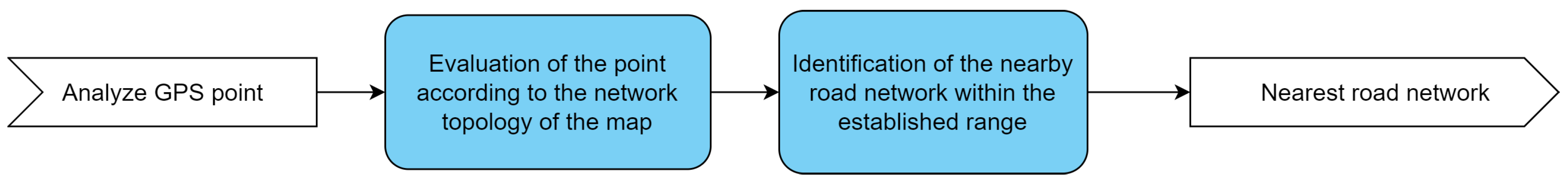
3.2. Road Network Information

The road network information uses the topology of points and polygons connected by vectors for the spatial analysis of GPS points over vehicular road networks in the areas where the data are being analyzed [47], as evidenced by the author of the present research [53]. For the calculation of the distance between the GPS coordinates and the network information it is proposed to use the great circle distance. A flow chart for network analysis is shown in Figure 2.

Figure 2. Flowchart of the GR Simplification algorithm for network analysis.

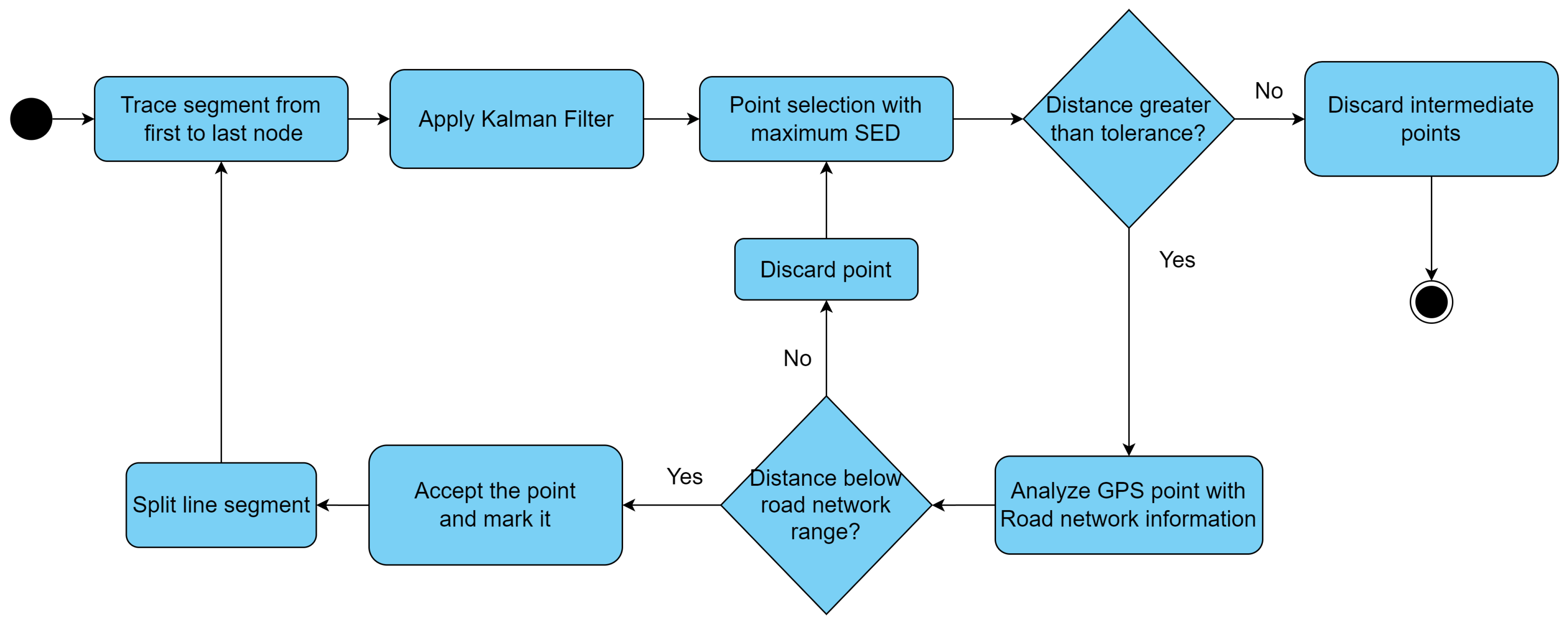
3.3. Simplification of GPS Points

The simplification is based on the simplification logic of the TD-TR algorithm, the Kalman noise reduction and the analysis of the road network information, in a hybrid way, to improve the presented results in the literature on the GPS trajectory simplification process. As a starting point, the simplification logic of Top Down Time Ratio is taken, a line is drawn between the first and last point of the trajectory and the Equations (9) and (10) are used to calculate the proposed intermediate points in the simplification logic.

$$x_i^{\prime }=x_s+\frac{t_i-t_s}{t_e-t_s}(x_e-x_s)$$

(9)

$$y_i^{\prime }=y_s+\frac{t_i-t_s}{t_e-t_s}(y_e-y_s)$$

(10)

For the calculation of the Synchronous Euclidean Distance (SED), the Equation (11).

$$SED=\sum _{i=1}^n\sqrt{{(x_{ti}-x_{ti}^{\prime })}^2+{(y_{ti}-y_{ti}^{\prime })}^2}$$

(11)

In the above expression, $(x_{ti},y_{ti})$ and $(x_{ti}^{\prime },y_{ti}^{\prime })$ represent the coordinates of a moving object in time $ti$ in the uncompressed and compressed traces respectively. In addition, n represents the total number of points considered.

The maximum distance point is selected, marked to hold, and compared with a threshold value. If the point is greater than the threshold value it is evaluated considering the network information. For this purpose the author of this paper proposes the evaluation of this point with the network information. This evaluation consists of comparing the distance between this point with the neighboring points that are part of the road network information, selecting the point with the greatest distance. If the distance from this point to the line segment is greater than the defined tolerance, the point is accepted; otherwise, if it is less, all points that are not marked are discarded. The simplification is executed as long as there are unanalyzed GPS trajectory points and as a result the simplified GPS trajectory is obtained. Figure 3 shows the simplification flowchart.

Figure 3. Flowchart of the GR Simplification algorithm for point simplification.

Brief Description of the Application of Point Simplification with Road Network Analysis

The simplification process of the proposed algorithm performs the application of the Kalman filter to the trajectory or segment being analyzed to then proceed to the simplification of the points. The points simplification process uses the logic of the TD-TR algorithm, which was selected as the basis for the proposal after performing an initial diagnosis in conjunction with other algorithms considered relevant by the author of this work; the logic of the TD-TR simplification process is taken as a basis in conjunction with the analysis of network information to reduce the number of points of the filtered trajectory and validate that these points are correct in the context of a vehicular road network. Simplification begins by plotting the segment, to which the Kalman filter will be applied to smooth the initial line segment between the first and last point. It then calculates by means of the synchronous Euclidean distance, the distances of all points to the line segment and identifies the point furthest from the line segment (or the maximum distance) and marks it to be kept. For this process, a obtained tolerance from the average of distances from one point to the next within the same trajectory has been selected. If the distance from the selected point to the line segment is less than the defined tolerance, all unmarked points are discarded, otherwise it selects the marked point to evaluate it with the network information and continues dividing the line segment with this point as shown in the Figure 4a. This procedure is executed recursively until the value is less than the tolerance or the line segment can no longer be divided.

Figure 4. Simplification process components: (a) Simplification of points using synchronous Euclidean distance. (b) Evaluation of a point with network information. (c) Network information associated with the street intersection.

In case the point is marked, it is evaluated with the network information to decide whether or not it can be added to the final simplified trajectory. To evaluate a marked point, the distance from the great-circle of the point to all points in the network is calculated using the Equation (12):

$$cos▵\sigma =(sin{b}_{1}sin{b}_2)+(cos{b}_{1}cos{b}_{2}cos\left|c\right|)$$

(12)

Two points $P_1(a_1,b_1)$ and $P_2(a_2,b_2)$ are used in the equation. Where $a_{1,2}$ and $b_{1,2}$ represent the longitudes and latitudes respectively in degrees and c represents the absolute value of the difference of the longitude axes $(a_1-a_2)$ between the respective coordinates. The above formula expresses the result as a difference of angles, so to obtain the distance with respect to the circumference of the planet the Equation (13) is used:

$$d=r▵\sigma$$

(13)

where d is the calculated arc length, r corresponds to the radius of the sphere representing the planet Earth and $▵\sigma$ is the central angle between two points.

A graphical representation of the simplification of the marked points and the evaluation with the points of the road networks is shown in Figure 4b.

The road network information is used to discard points that are not within a lane on a road, a lane width of 4.5 m has been considered for this work. As shown in Figure 4c the points of the trajectory $P_2$ and $P_3$ are eliminated keeping those that are in the lane width, thus keeping only the necessary points to trace the trajectory of a vehicle without affecting its correct representation.

The greater the width of the lane, the greater the possibility of accepting more points. The use of the great-circle distance in the analysis of network information allows more accurate calculations, since the distance between two points in Euclidean space is the length of a straight line between them, but on the sphere there are no straight lines. In spaces with curvature, straight lines are replaced by geodesics. Geodesics on the sphere are circles on the sphere whose centers coincide with the center of the sphere, and are called great circles [54].

The computational complexity in the proposed approach is $O\left(n^2\right)$. This is because the TD-TR algorithm is derived from the original Douglas-Peucker algorithm, and unlike an $O\left(nlo{g}_n\right)$ implementation improvement that can be applied to Douglas-Peucker, this improvement cannot be employed in TD-TR due to its particular geometric properties.

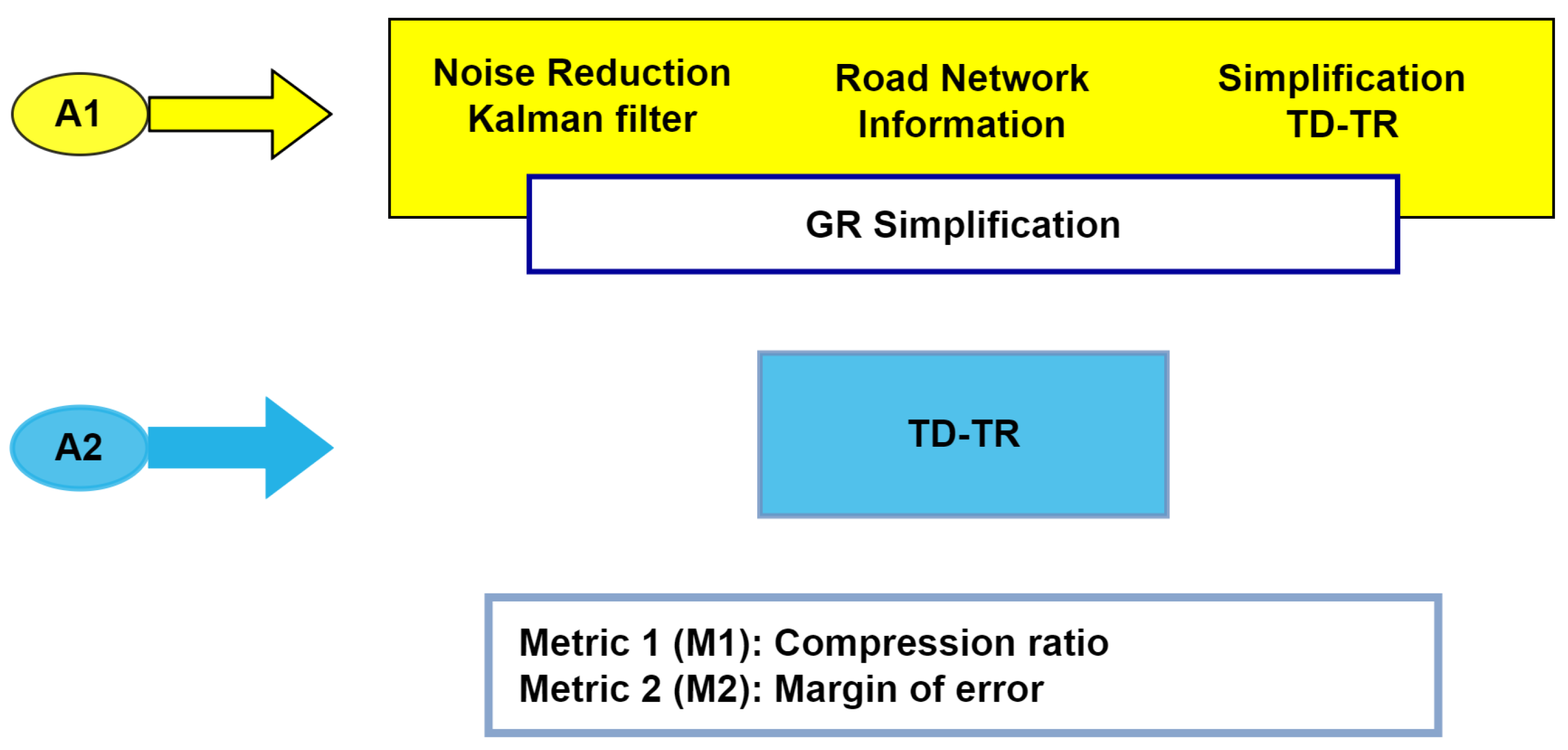
3.4. Initial Experiment

In this experiment a trajectory with 8067 points is taken, to check the changes in the data from the application of the phases of the GR algorithm.

As inputs in this experiment we have a GPS trajectory and as output we obtain the compressed trajectory. Initially the data is filtered in the simplification phase by applying noise reduction to deal with the noise present in the trajectory. This means a change in the input data due to the decrease of the noise present in the trajectory or segment. Subsequently the filtered data are analyzed with the network information to discard redundant points and select the ones that are going to be part of the simplified trajectory. Table 2 shows the results obtained from the application of the algorithm.

Table 2. Results of the initial experiment for the stages of the GR algorithm.

Phases	Description	Number of Points	Size in Disc of the Trajectory Result
Original trajectory	Trajectory without any processing	8067	668 kb
Simplification phase	Simplification, Kalman filter and road network information	578	47 kb

The original trajectory has 8067 points and occupies 668 kb of disk space. After applying the GR algorithm the number of end points of the path is 578, occupying only 47 kb of disk space. The compression ratio for this case is 92.84%.

The implementation of the proposed algorithm in a controlled environment is available from a public repository (Source code available at https://github.com/gary-reyes-zambrano/Algoritmo-de-simplificacion-GR (accessed on 22 August 2022)).

4. Results

4.1. Used Data

4.1.1. Geolife

The “Geolife (Microsoft Research Asia)” dataset [55] consists of information from 182 users over a period of more than three years from April 2007 to August 2012. The GPS trajectories of this dataset contains the information of: “latitude”, “longitude”, “altitude”, “time” of each user record. The time is taken considering the GMT standard. This dataset contains 17.621 trajectories with a total distance of about 1.2 million km and a total duration of more than 48.000 h. These trajectories were recorded by different GPS loggers and GPS phones, and have a variety of sampling rates.

4.1.2. Mobile Century

The data set used “Mobile Century” data [56] collected on 8 February 2008 between 10 a.m. and 6 p.m. on Interstate 880, CA as part of a joint UC Berkeley-Nokia project funded by the Department of Transportation to support exploration of the use of GPS-enabled sensor phones to monitor traffic. This data consists of individual “trips” in one direction on Interstate 880. Northbound trips are in the “NB_veh_files” folder and southbound trips are in the “SB_veh_files” folder. Each file contains the following five columns: “unixtime”, “latitude”, “longitude”, “postmile” and “speed”.

4.2. Initial Diagnostics of Batch GPS Trajectory Simplification Algorithms

To evaluate the simplification algorithms in terms of processing time, compression ratio and margin of error, the author of this paper used two significant samples of GPS trajectory databases as follows:

From the “Mobile Century” dataset a sample of 100,169 spatial coordinates is used, which represent 10.95% of the original database data. A sample of 340 trajectories was used out of a total of 2977 trajectories. For the selection of the sample, an area of approximately 24.51 × 24.45 km was delimited and the systematic sampling technique was used.

A sample of 417,056 spatial coordinates is used from the “Geolife Trajectories” dataset, which represents 1.68% of the original base size. A sample of 376 trajectories was used out of a total of 18,549 trajectories. For the selection of the sample, an area covering approximately 148.45 × 137.85 km was delimited, the same area where there is the highest concentration of trajectories, which would allow discarding many trajectories containing atypical points, and the systematic sampling technique was used.

For the initial diagnosis, the algorithms considered relevant by the author of this work were selected after the literature review; the algorithms were run on the samples obtained for the two data sets. A summary is shown in Table 3, showing the mean of the results obtained for each algorithm.

Table 3. Average of the results of the initial diagnosis of the simplification algorithms on the selected samples.

Algorithm	Processing Time (Seconds)	Compression Ratio (Percentage)	Margin of Error (Kilometers)
Douglas-Peucker	15,011.75	91.60	13.88
Lang	3159.65	76.19	4.75
Visvalingam	214.70	67.07	0.09
TD-TR	13,852.44	86.01	0.80

The obtained results in the initial diagnostic study led to the conclusion that:

• The Visvalingam algorithm shows the worst compression ratio rates, being a very unstable algorithm in its behavior before different data sets;
• The TD-TR algorithm is the second algorithm with the best compression ratio rate with an average of 86.01;
• Douglas-Peucker obtains the best results in terms of compression ratio, however the processing time is longer than TD-TR and the margin of error is also higher, being 13.88 km while TD-TR presents 0.80 km;
• The TD-TR algorithm is proposed in the literature as an improvement to the Douglas Peucker algorithm and presents better results in terms of margin of error and processing time.

As a result of the initial diagnosis in the present work, the TD-TR simplification logic is selected as the basis for the elaboration of the proposal. The author of the present work considers that it is the best option of the four algorithms analyzed, since it reported the second best compression ratio, the second best margin of error, considering that it is the only one that performs a spatio-temporal analysis and that the applicability of the present work is not based on the analysis of real-time trajectories, which are more focused on obtaining better times. The used metrics to perform the measurements to the “GR Simplification” algorithm, considering the application scenario in road networks and disconnected (batch) environments, are the compression ratio rate and the margin of error [28,57,58]. For the comparison of the “GR Simplification” algorithm and TD-TR, the margin of error formula found in this paper [59] is used.

4.3. Obtained Results from the GR Simplification Algorithm for GPS Trajectory Simplification

To perform the measurements, the proposed algorithm “GR Simplification” was implemented in R language, which uses Kalman filtering logic, TD-TR simplification logic and road network information.

From the Datasets two samples are chosen whose trajectories are selected systematically, each sample uses the data corresponding to the GeoLife and Mobile Century datasets, with the following characteristics:

• Sample 1 (Geolife): three hundred and seventy-six trajectories, each containing between 1 and 18.924 points;
• Sample 2 (Mobile Century): three hundred and forty trajectories, each containing between 17 and 8.067 points.

In the two samples, the trajectories are selected systematically.

The calculations of the compression ratio and margin of error metrics were performed and a comparison is established with the obtained results by the TD-TR algorithm, as shown in Figure 5.

Figure 5. Comparison: GR Simplification vs. TD-TR.

After performing the measurements in which the “GR Simplification” (denoted A1) and “TD-TR” (denoted A2) algorithms are executed, obtaining the values of compression ratio (metric 1) and margin of error (metric 2) for both algorithms, the average of the results, for the two samples, are shown in the Table 4. The obtained results are validated using the corresponding statistical tests.

Table 4. Comparison of the average obtained results between the TD-TR and GR algorithms.

	Compression Ratio (Percentage)		Margin of Error (Meters)
	TD-TR	GR	TD-TR	GR
Sample 1 (Geolife)	85.485	90.214	14.22	6.47
Sample 2 (Mobile Century)	92.787	93.395	3.69	2.77
Average	89.136	91.804	8.955	4.62

The values presented in the Table 5 compare the execution times between GR algorithm and TD-TR algorithm, on two geospatial datasets: Geolife and Mobile Century. On both datasets, GR proves to be competitive in terms of run time, with results varying by dataset. This suggests that the GR algorithm offers an efficient solution for geospatial data simplification in various scenarios.

Table 5. Comparison of simplification algorithm execution times (times are expressed in seconds).

Algorithms	Geolife	Mobile Century
TD-TR	6982.980	1734.965
GR	4074.080	1666.680

5. Discussion

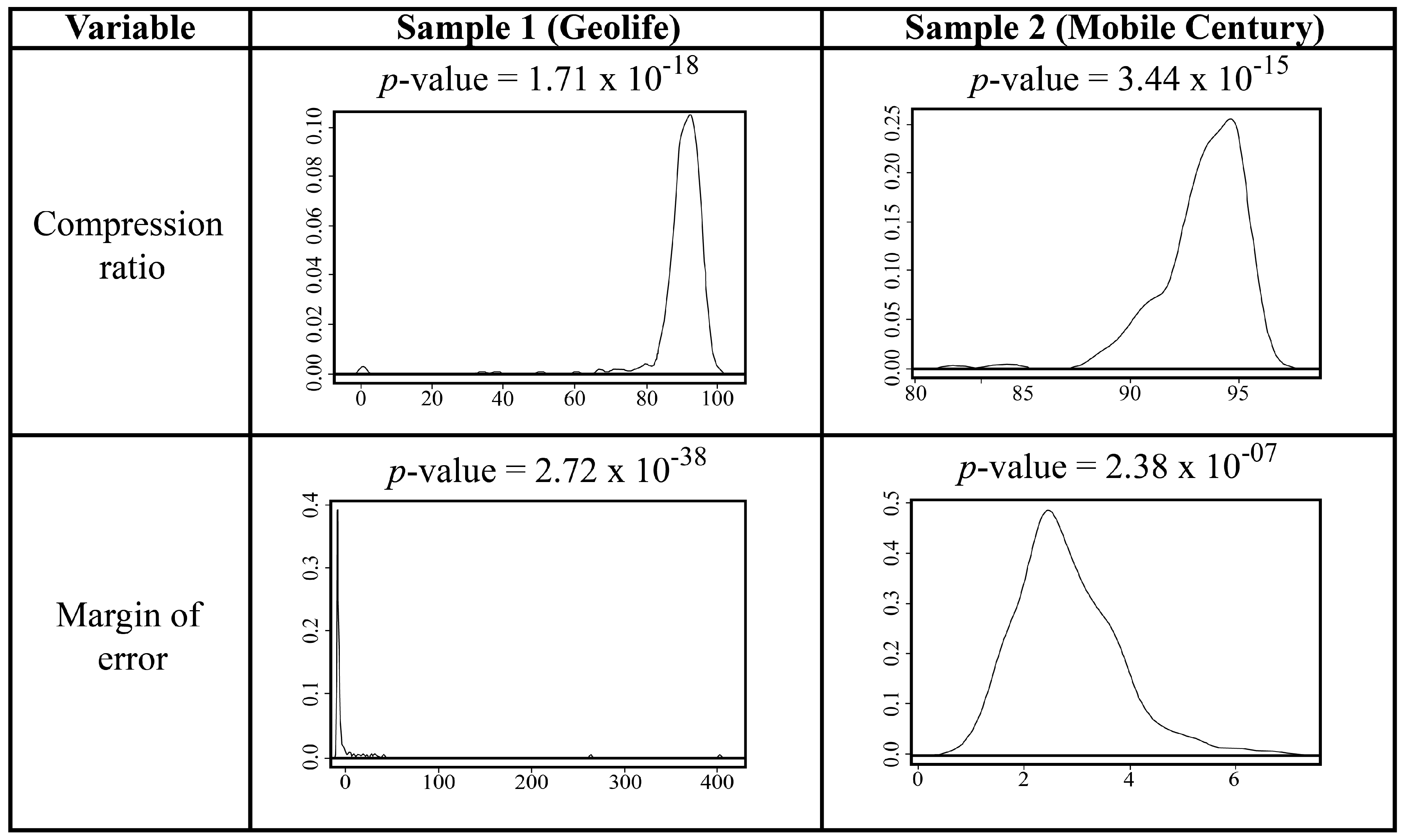
5.1. Assumption of Normality

There are several methods for testing the fit to the normal distribution, among the best known are the Kolmogorov-Smirnov and Shapiro-Wilk’s test [60]. The latter, in the author’s opinion, is widely recommended and is used in the present work.

The null hypothesis ($H_0$) for validation is defined as “the groups of samples fit a normal distribution”, so that if the test yields a significant difference there is no fit to the normal distribution.

The Table 6 shows the obtained results after performing two tests to check the assumption of normality, both for the compression ratio metric and the margin of error metric.

Table 6. Shapiro-Wilk’s test results for the selected samples.

Tests	GR (Ratio of Compression)	GR (Margin of Error)	TD-TR (Ratio of Compression)	TD-TR (Margin of Error)
Sample 1 (Geolife)	Rejected $H_0$	Rejected $H_0$	Rejected $H_0$	Rejected $H_0$
Sample 2 (Mobile Century)	Rejected $H_0$	Rejected $H_0$	Rejected $H_0$	Rejected $H_0$

When performing the Shapiro-Wilk’s test on the vectors, to check the assumption of normality of the obtained results in the compression ratio metric, it is evident that the values do not conform to a normal distribution; therefore, the null hypothesis ($H_0$) is rejected. In the same way it is observed that when performing the test to check the assumption of normality for the margin of error, it is evident that the values of the sample do not conform to a normal distribution, therefore the null hypothesis ($H_0$) is rejected. This can be seen visually by observing the p-value values and the density plots in Figure 6 and Figure 7.

Figure 6. Density plot of the obtained results with the GR algorithm.

Figure 7. Density plot of the obtained results with the TD-TR algorithm.

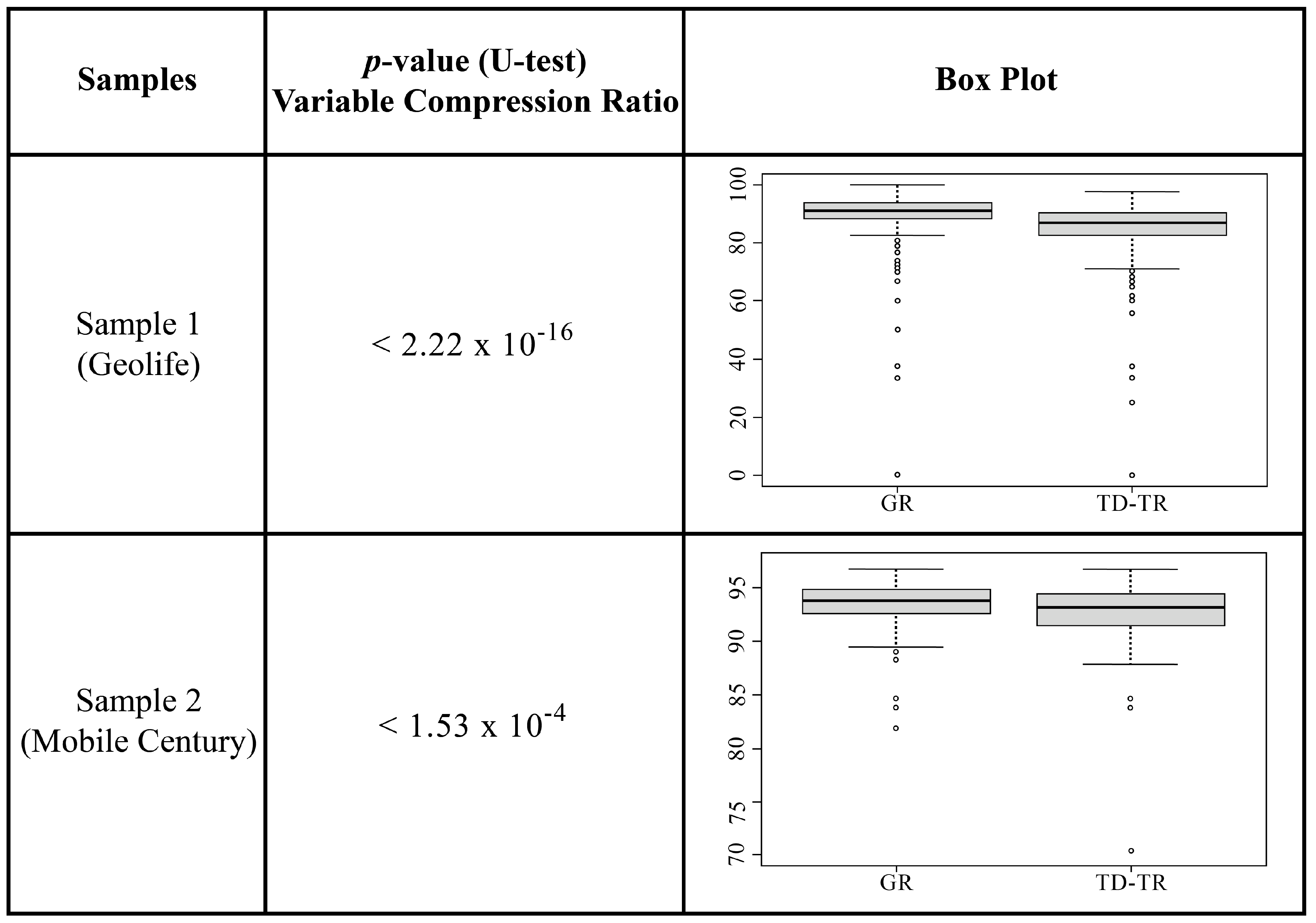
5.2. Analysis of Results for Compression Ratio Metric

The Mann-Whitney test is a nonparametric test that allows comparison of two independent samples that do not conform to a normal distribution, as is the case for measurements made for the compression ratio in the two samples of the data sets. Three researchers, Mann, Whitney and Wilcoxon, separately refined a very similar nonparametric test that can determine whether samples can be considered identical or not on the basis of their ranges [61,62].

The result of applying this test to the two samples with respect to the compression ratio can be seen in Figure 8.

Figure 8. Mann-Whitney test results for compression ratio.

It is observed that all the values (p-values) are less than 0.05, which means that there are significant differences according to the test applied with a 95% confidence level, a obtained result for the two samples. Visual inspection shows that the median values are higher for the GR Simplification.

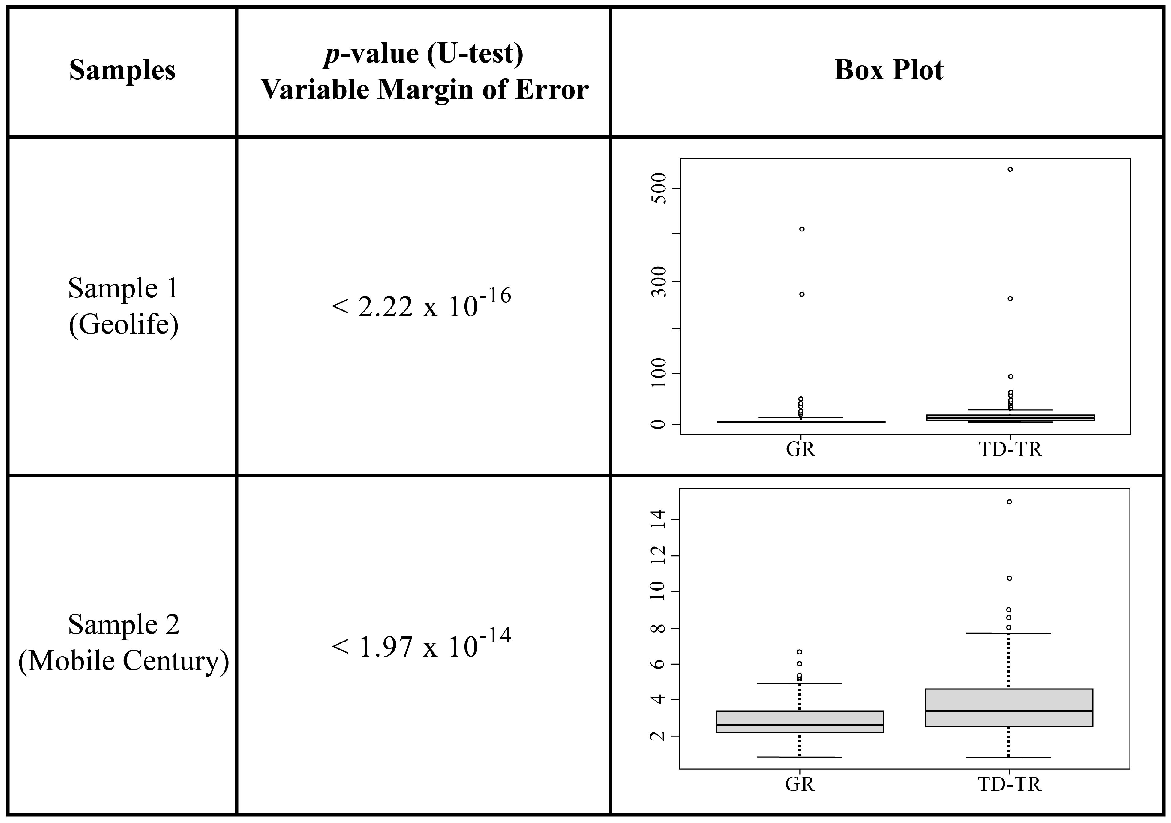
5.3. Analysis of Results for the Margin of Error Metric

To check whether the samples are identical, the nonparametric Mann-Whitney test (U-test) is applied. This test is applied in the present work to check that the samples are identical and thus verify the veracity of the results. The result of the application of this test for the two samples with respect to the margin of error can be seen in the Figure 9.

Figure 9. Results of Mann-Whitney tests for margin of error.

It is observed that all the values (p-values) are less than 0.05, which means that there are significant differences according to the applied test with a 95% confidence, obtained result for the two samples. Visual inspection shows that the median values are lower for the GR Simplification.

After performing the validation and hypothesis test on metric 1: compression ratio, it can be seen that there are significant differences between the “GR Simplification” and “TD-TR” algorithms. The box plots show that the median values are higher for “GR Simplification”. After performing the validation and hypothesis test on metric 2: margin of error, it is found that the means of the groups being compared have significant differences. The box plots show that the median values are lower for the “GR Simplification”. All tests are performed for 95% confidence.

It is evident that the compression ratio of the GR Simplification is better with respect to the TD-TR simplification. It is evident that the margin of error is lower, comparing the GR Simplification with respect to the TD-TR simplification.

6. Conclusions

The algorithm “GR Simplification” developed as a result of the present work, allows the simplification of GPS trajectory points, based on noise reduction, trajectory simplification and network information, increasing the data compression ratio compared to the TD-TR algorithm.

The measurements performed show that the GR trajectory simplification algorithm, based on noise reduction, trajectory simplification and network information proposed in this research, presents a higher compression ratio and even improves the margin of error with respect to its similar ones analyzed in the literature.

The validation of the obtained results through statistical tests allowed verifying that there is an increase in the compression ratio.

The results obtained from the “GR Simplification” algorithm show that it can be used in the processing of vehicle trajectories that have available information from the road network, allowing GPS trajectory analysis applications to optimally manage their storage space.

Specific targeting of each component leads to promising opportunities in fields such as logistics, fleet tracking, urban planning, and environmental monitoring. Enhancing data compression and accuracy has the potential to optimize resources in these strategic areas, and this algorithm could play a crucial role in doing so.

To boost results and research efficiency, key practices are suggested. Improving data quality through data cleaning and preprocessing, such as the use of routing techniques for correction of trajectories with anomalous points, can increase accuracy. Exploring varied and representative data sets will provide a more complete view of algorithm applicability. Adopting optimization and parallelization techniques will reduce processing times and allow large sets to be handled. Together, these strategies will enrich the research and increase the quality of the results obtained.

Despite the advances of the “GR Simplification” algorithm, it is crucial to note its current limitations. The implementation may face constraints in terms of processing time when dealing with large data sets. Accuracy is linked to the quality of road network data. Although the algorithm is effective compared to others, its usefulness depends on the context and type of GPS trajectories analyzed.

In addition, it is important to note that the data utilized in this study were obtained more than 10 years ago, which may limit the relevance of the factors analyzed. It is recommended to utilize more up-to-date datasets to reflect current conditions and more accurately capture characteristic patterns.

As lines of future work, it is proposed to improve the processing time of the GR Simplification algorithm, through a new implementation that considers a parallel processing approach of several trajectories. We also propose an implementation that includes the Kalman filter logic and the use of networks for online GPS trajectory simplification algorithms, considering the use of a temporary storage memory.

References

1. Wang, H.; Wu, Z.; Chen, J.; Chen, L. Evaluation of road traffic noise exposure considering differential crowd characteristics. Transp. Res. Part D Transp. Environ. 2022, 105, 103250. [Google Scholar] [CrossRef]
2. Chen, J.; Xu, M.; Xu, W.; Li, D.; Peng, W.; Xu, H. A Flow Feedback Traffic Prediction Based on Visual Quantified Features. IEEE Trans. Intell. Transp. Syst. 2023, 24, 10067–10075. [Google Scholar] [CrossRef]
3. Muckell, J.; Patil, V.; Ping, F.; Hwang, J.H.; Lawson, C.T.; Ravi, S.S. SQUISH: An online approach for GPS trajectory compression. In Proceedings of the 2nd International Conference and Exhibition on Computing for Geospatial Research & Application, Washington, DC, USA, 23–25 May 2011; pp. 1–8. [Google Scholar] [CrossRef]
4. Corcoran, P.; Mooney, P.; Huang, G. Unsupervised trajectory compression. In Proceedings of the 2016 IEEE International Conference on Robotics and Automation (ICRA), Stockholm, Sweden, 16–21 May 2016; pp. 3126–3132. [Google Scholar] [CrossRef]
5. Rana, R.; Yang, M.; Wark, T.; Chou, C.T.; Hu, W. Simpletrack: Adaptive trajectory compression with deterministic projection matrix for mobile sensor networks. IEEE Sens. J. 2015, 15, 365–373. [Google Scholar] [CrossRef]
6. Trajcevski, G. Compression of Spatio-temporal Data. In Proceedings of the 2016 17th IEEE International Conference on Mobile Data Management (MDM), Porto, Portugal, 13–16 June 2016; pp. 4–7. [Google Scholar] [CrossRef]
7. Chen, Y.; Yu, P.; Chen, W.; Zheng, Z.; Guo, M. Embedding-Based Similarity Computation for Massive Vehicle Trajectory Data. IEEE Internet Things J. 2022, 9, 4650–4660. [Google Scholar] [CrossRef]
8. Bashir, M.; Ashraf, J.; Habib, A.; Muzammil, M. An intelligent linear time trajectory data compression framework for smart planning of sustainable metropolitan cities. Trans. Emerg. Telecommun. Technol. 2022, 33, e3886. [Google Scholar] [CrossRef]
9. Wang, Y.; Zhang, Z.; Liu, D. An optimization model for the transportation network with hierarchical structure: The case of China Post. J. Ambient. Intell. Humaniz. Comput. 2019, 12, 167–182. [Google Scholar] [CrossRef]
10. Richter, K.F.; Schmid, F.; Laube, P. Semantic trajectory compression: Representing urban movement in a nutshell. J. Spat. Inf. Sci. 2012, 4, 3–30. [Google Scholar] [CrossRef]
11. Souza, J.C.S.D.; Assis, T.M.L.; Pal, B.C. Data Compression in Smart Distribution Systems via Singular Value Decomposition. IEEE Trans. Smart Grid 2017, 8, 275–284. [Google Scholar] [CrossRef]
12. Muckell, J.; Olsen, P.W.; Hwang, J.H.; Lawson, C.T.; Ravi, S.S. Compression of trajectory data: A comprehensive evaluation and new approach. GeoInformatica 2014, 18, 435–460. [Google Scholar] [CrossRef]
13. Nibali, A.; He, Z. Trajic: An Effective Compression System for Trajectory Data. IEEE Trans. Knowl. Data Eng. 2015, 27, 3138–3151. [Google Scholar] [CrossRef]
14. Alowayr, A.D.; Alsalooli, L.A.; Alshahrani, A.M.; Akaichi, J. A review of trajectory data mining applications. In Proceedings of the 2021 International Conference of Women in Data Science at Taif University, WiDSTaif 2021, Taif, Saudi Arabia, 30–31 March 2021. [Google Scholar] [CrossRef]
15. Mazimpaka, J.D.; Timpf, S. Trajectory data mining: A review of methods and applications. J. Spat. Inf. Sci. 2016, 2016, 61–99. [Google Scholar] [CrossRef]
16. Ji, Y.; Liu, H.; Liu, X.; Ding, Y.; Luo, W. A comparison of road-network-constrained trajectory compression methods. In Proceedings of the 2016 IEEE 22nd International Conference on Parallel and Distributed Systems (ICPADS), Wuhan, China, 13–16 December 2016; pp. 256–263. [Google Scholar] [CrossRef]
17. Ouyang, Z.; Xue, L.; Ding, F.; Li, D. PSOTSC: A Global-Oriented Trajectory Segmentation and Compression Algorithm Based on Swarm Intelligence. ISPRS Int. J. Geo-Inf. 2021, 10, 817. [Google Scholar] [CrossRef]
18. Chen, H.; Chen, X. A Trajectory Ensemble-Compression Algorithm Based on Finite Element Method. ISPRS Int. J. Geo-Inf. 2021, 10, 334. [Google Scholar] [CrossRef]
19. Song, J.; Miao, R. A Novel Evaluation Approach for Line Simplification Algorithms towards Vector Map Visualization. ISPRS Int. J. Geo-Inf. 2016, 5, 223. [Google Scholar] [CrossRef]
20. Zheng, Y. Trajectory data mining: An overview. ACM Trans. Intell. Syst. Technol. 2015, 6, 1–41. [Google Scholar] [CrossRef]
21. Wang, S.; Zhong, E.; Li, K.; Song, G.; Cai, W. A Novel Dynamic Physical Storage Model for Vehicle Navigation Maps. ISPRS Int. J. Geo-Inf. 2016, 5, 53. [Google Scholar] [CrossRef]
22. Amigo, D.; Pedroche, D.S.; García, J.; Molina, J.M. Review and classification of trajectory summarisation algorithms: From compression to segmentation. Int. J. Distrib. Sens. Netw. 2021, 17, 15501477211050729. [Google Scholar] [CrossRef]
23. Salomon, D. Data Compression: The Complete Reference, 4th ed.; Springer: Berlin/Heidelberg, Germany, 2014; pp. 1–1093. [Google Scholar] [CrossRef]
24. Gudmundsson, J.; Katajainen, J.; Merrick, D.; Ong, C.; Wolle, T. Compressing spatio-temporal trajectories. Comput. Geom. Theory Appl. 2009, 42, 825–841. [Google Scholar] [CrossRef]
25. Lv, C.; Chen, F.; Xu, Y.; Song, J.; Lv, P. A trajectory compression algorithm based on non-uniform quantization. In Proceedings of the 2015 12th International Conference on Fuzzy Systems and Knowledge Discovery (FSKD), Zhangjiajie, China, 15–17 August 2015; pp. 2469–2474. [Google Scholar] [CrossRef]
26. Liu, D.; Wang, T.; Li, X.; Ni, Y.; Li, Y.; Jin, Z. A Multiresolution Vector Data Compression Algorithm Based on Space Division. ISPRS Int. J. Geo-Inf. 2020, 9, 721. [Google Scholar] [CrossRef]
27. Meratnia, N.; Rolf, A.; ITC, E. A New Perspective on Trajectory Compression Techniques; International Society for Photogrammetry and Remote Sensing (ISPRS): Quebec City, QC, Canada, 2003; pp. 2–3. [Google Scholar]
28. Zheng, Y.; Zhou, X. Computing with Spatial Trajectories; Springer: Berlin/Heidelberg, Germany, 2011; pp. 1–306. [Google Scholar] [CrossRef]
29. Lin, X.; Ma, S.; Zhang, H.; Wo, T.; Huai, J. One-pass error bounded trajectory simplification. Proc. VLDB Endow. 2017, 10, 841–852. [Google Scholar] [CrossRef]
30. Feldman, D.; Sugaya, A.; Rus, D. An effective coreset compression algorithm for large scale sensor networks. In Proceedings of the 2012 ACM/IEEE 11th International Conference on Information Processing in Sensor Networks (IPSN), Beijing, China, 16–20 April 2012; pp. 257–268. [Google Scholar] [CrossRef]
31. Wang, Z.; Long, C.; Cong, G.; Zhang, Q. Error-Bounded Online Trajectory Simplification with Multi-Agent Reinforcement Learning. In Proceedings of the ACM SIGKDD International Conference on Knowledge Discovery and Data Mining, Singapore, 14–18 August 2021; pp. 1758–1768. [Google Scholar] [CrossRef]
32. Li, S.; Zhang, K.; Yin, H.; Yin, D.; Zu, H.; Gao, H. ROPW: An Online Trajectory Compression Algorithm. Lect. Notes Comput. Sci. 2021, 12680 LNCS, 16–28. [Google Scholar] [CrossRef]
33. Hendawi, A.M.; Khot, A.; Rustum, A.; Basalamah, A.; Teredesai, A.; Ali, M. A Map-Matching Aware Framework for Road Network Compression. In Proceedings of the 2015 16th IEEE International Conference on Mobile Data Management, Pittsburgh, PA, USA, 15–18 June 2015; Volume 1, pp. 307–310. [Google Scholar] [CrossRef]
34. Hussain, S.A.; Hassan, M.U.; Nasar, W.; Ghorashi, S.; Jamjoom, M.M.; Abdel-Aty, A.H.; Parveen, A.; Hameed, I.A. Efficient Trajectory Clustering with Road Network Constraints Based on Spatiotemporal Buffering. ISPRS Int. J. Geo-Inf. 2023, 12, 117. [Google Scholar] [CrossRef]
35. Song, R.; Sun, W.; Zheng, B.; Zheng, Y. A novel framework of trajectory compression in road networks. Proc. VLDB Endow. 2014, 7, 661–672. [Google Scholar] [CrossRef]
36. Hunnik, R.V. Extensive Comparison of Trajectory Simplification Algorithms. Master’s Thesis, Utrecht University, Utrecht, The Netherlands, 2017; pp. 1–22. [Google Scholar]
37. Lin, C.Y.; Hung, C.C.; Lei, P.R. A velocity-preserving trajectory simplification approach. In Proceedings of the 2016 Conference on Technologies and Applications of Artificial Intelligence (TAAI), Hsinchu, Taiwan, 25–27 November 2016; pp. 58–65. [Google Scholar] [CrossRef]
38. Kellaris, G.; Pelekis, N.; Theodoridis, Y. Trajectory Compression under Network Constraints; Springer: Berlin/Heidelberg, Germany, 2009; pp. 392–398. [Google Scholar] [CrossRef]
39. Gomez-Gil, J.; Ruiz-Gonzalez, R.; Alonso-Garcia, S.; Gomez-Gil, F.J. A Kalman filter implementation for precision improvement in Low-Cost GPS positioning of tractors. Sensors 2013, 13, 15307–15323. [Google Scholar] [CrossRef] [PubMed]
40. Ivanov, R. Real-time GPS track simplification algorithm for outdoor navigation of visually impaired. J. Netw. Comput. Appl. 2012, 35, 1559–1567. [Google Scholar] [CrossRef]
41. Chen, C.; Ding, Y.; Guo, S.; Wang, Y. DAVT: An Error-Bounded Vehicle Trajectory Data Representation and Compression Framework. IEEE Trans. Veh. Technol. 2020, 69, 10606–10618. [Google Scholar] [CrossRef]
42. Meratnia, N.; By, R.A.D. Spatiotemporal compression techniques for moving point objects. Lect. Notes Comput. Sci. 2004, 2992, 765–782. [Google Scholar] [CrossRef]
43. Whyatt, J.D.; Wade, P.R. The Douglas-Peucker line simplification algorithm. Bull. Soc. Univ. Cartogr. 1988, 22, 17–25. [Google Scholar]
44. Visvalingam, M.; Whyatt, J.D. Line generalisation by repeated elimination of points. Cartogr. J. 1993, 30, 46–51. [Google Scholar] [CrossRef]
45. Buchin, M.; Driemel, A.; Van Kreveld, M.; Sacristan, V. Segmenting trajectories: A framework and algorithms using spatiotemporal criteria. J. Spat. Inf. Sci. 2011, 3, 33–63. [Google Scholar] [CrossRef]
46. Bach, T.; Li, T.; Huang, R.; Chen, L.; Jensen, C.S.; Pedersen, T.B. Compression of Uncertain Trajectories in Road Networks. PVLDB 2020, 13, 1050–1063. [Google Scholar] [CrossRef]
47. Weiss, R.; Weibel, R. Road network selection for small-scale maps using an improved centrality-based algorithm. J. Spat. Inf. Sci. 2014, 31, 71–99. [Google Scholar] [CrossRef]
48. Koegel, M.; Baselt, D.; Mauve, M.; Scheuermann, B. A comparison of vehicular trajectory encoding techniques. In Proceedings of the 2011 The 10th IFIP Annual Mediterranean Ad Hoc Networking Workshop, Favignana Island, Italy, 12–15 June 2011; pp. 87–94. [Google Scholar] [CrossRef]
49. Lawson, C.T. Compression and Mining of GPS Trace Data: New Techniques and Applications. In Final Report: Region II University Transportation Research Center; City University of New York, University Transportation Research Center: New York, NY, USA, 2011; pp. 1–25. [Google Scholar]
50. Reyes, G. Algoritmo de Compresión de Trayectorias GPS Basado en el Algoritmo Top Down Time Ratio (TD-TR). In Proceedings of the 2017 V Congreso Científico Internacional, Tecnología Universidad Sociedad, Samborondón, Ecuador, 8–10 November 2017; pp. 194–204. Available online: https://www.ecotec.edu.ec/content/uploads/investigacion/tus/2017-memorias-TUS.pdf (accessed on 24 January 2022).
51. Reyes, G.; Estrada, V. Comparison Analysis On Noise Reduction In Gps Trajectories Simplification; Latin American and Caribbean Consortium of Engineering Institutions: Boca Raton, FL, USA, 2021. [Google Scholar] [CrossRef]
52. Lin, K.; Xu, Z.; Qiu, M.; Wang, X.; Han, T. Noise filtering, trajectory compression and trajectory segmentation on GPS data. In Proceedings of the 2016 11th International Conference on Computer Science & Education (ICCSE), Nagoya, Japan, 23–25 August 2016; pp. 490–495. [Google Scholar] [CrossRef]
53. Reyes, G.; Crespo, C.; León-Granizo, O.; Bazán, W.; Horta, R. Propuesta de método de extracción de ubicaciones georreferenciales de una red de carreteras para el análisis de trayectorias GPS Proposal for a method to extract georeferenced locations from a road network for the analysis of GPS trajectories. Investig. Tecnol. Innov. 2022, 14, 1–15. [Google Scholar]
54. Fenn, R. Spherical Geometry. In Geometry; Springer: London, UK, 2001; pp. 253–285. [Google Scholar] [CrossRef]
55. Zheng, Y.; Zhang, L.; Xie, X.; Ma, W.Y. Mining Interesting Locations and Travel Sequences From GPS Trajectories. In Proceedings of the 2009 Proceedings of the 18th International Conference on World Wide Web, Madrid, Spain, 20–24 April 2009; pp. 791–800. [Google Scholar] [CrossRef]
56. Herrera, J.; Work, D.; Herring, R.; Ban, X.; Jacobson, Q.; Bayen, A. Evaluation of traffic data obtained via GPS-enabled mobile phones: The Mobile Century field experiment. Transp. Res. C Emerg. Technol. 2010, 18, 568–583. [Google Scholar] [CrossRef]
57. Reyes, G.; Maquilón, V.; Estrada, V. Relationships of Compression Ratio and Error in Trajectory Simplification Algorithms; Springer International Publishing: Cham, Switzerland, 2021; pp. 140–155. [Google Scholar]
58. Muckell, J.; Olsen, P.W.; Hwang, J.H.; Ravi, S.S.; Lawson, C.T. A framework for efficient and convenient evaluation of trajectory compression algorithms. In Proceedings of the 2013 Fourth International Conference on Computing for Geospatial Research and Application, San Jose, CA, USA, 22–24 July 2013; pp. 24–31. [Google Scholar] [CrossRef]
59. Liu, M.; He, G.; Long, Y. A Semantics-Based Trajectory Segmentation Simplification Method. J. Geovis. Spat. Anal. 2021, 5, 19. [Google Scholar] [CrossRef]
60. Tapia, C.; Flores, K. Pruebas para comprobar la normalidad de datos en procesos productivos: Anderson-Darling, Ryan-Joiner, Shapiro-Wilk y Kologórov-Smirnov. Soc. Rev. Cienc. Soc. Hum. 2021, 23, 83–97. [Google Scholar]
61. Saldaña, M.R. Contraste de Hipótesis Comparación de dos medias independientes mediante pruebas no paramétricas: Prueba U de Mann-Whitney - Dialnet. Rev. EnfermeríaTrab. 2013, 3, 77–84. [Google Scholar]
62. Guillen, A.; A Araiza, L.; Cerna, E.; Valenzuela, J.; Uanl, J.L.; Nicolás, S.; Coah, S. Métodos No-Paramétricos de Uso Común ( Non Parametric Methods of Common Usage ). DAENA Int. J. Good Conscienc. 2012, 7, 132–155. [Google Scholar]
Disclaimer/Publisher’s Note: The statements, opinions and data contained in all publications are solely those of the individual author(s) and contributor(s) and not of MDPI and/or the editor(s). MDPI and/or the editor(s) disclaim responsibility for any injury to people or property resulting from any ideas, methods, instructions or products referred to in the content.
Article Metrics
Citations
Article Access Statistics
Multiple requests from the same IP address are counted as one view.