Soft Integration of Geo-Tagged Data Sets in J-CO-QL⁺

Abstract

The possibility offered by the current technology to collect and store data sets regarding public places located on the Earth globe is posing new challenges, as far as the integration of these data sets is concerned. Analysts usually need to perform such an integration from scratch, without performing complex and long preprocessing or data-cleaning tasks, as well as without performing training activities that require tedious and long labeling of data; furthermore, analysts now have to deal with the popular JSON format and with data sets stored within JSON document stores. This paper demonstrates that a methodology based on soft integration (i.e., data integration performed through soft computing and fuzzy sets) can now be effectively applied from scratch, through the J-CO Framework, which is a stand-alone tool devised to process JSON data sets stored within JSON document stores, possibly by performing soft querying on data sets. Specifically, the paper provides the following contributions: (1) It presents a soft-computing technique for integrating data sets describing public places, without any preliminary pre-processing, cleaning and training, which can be applied from scratch; (2) it presents current capabilities for soft integration of JSON data sets, provided by the J-CO Framework; (3) it demonstrates the effectiveness of the soft integration technique; (4) it shows how a stand-alone tool able to support soft computing (as the J-CO Framework) can be effective and efficient in performing data-integration tasks from scratch.

1. Introduction

Integrating geo-spatial information has become a crucial task in the current world. In fact, in the era of Open Data and Big Data, a plethora of sources can provide both authoritative and non-authoritative data sets concerning places. The situation is further complicated by the fact that social media provide people with tools for describing places in a non-controlled way. For example, Facebook provides its users with the functionality to define a “page”; a specific category of the page describes a “public place”, such as restaurants, pubs, air dressers, universities, parks and so on; through its API (Application Programming Interface), pages could be queried, on the basis of their category, location, coordinates, and so on. Another interesting service is called Google Places: it is a sub-service of Google Maps; Google Places API can be used to query its corpus to find places of interest, on the basis of category, location, and so on; this corpus is built by Google Maps by integrating both authoritative and non-authoritative data, these latter ones given by users through the social interface provided by Google Maps.

In the current scenario, it is very easy to collect data sets from multiple sources, such that these data sets provide geo-tagged information about public places. Since current APIs of social media and Open-Data portals provide data as (possibly) geo-tagged JSON documents (JSON stands for JavaScript Object Notation, see [1]), JSON document stores are the natural storage where to save such data sets. Consequently, integrating geo-tagged data sets describing public places asks for suitable tools, which are able to work on JSON document stores. This is the reason why at University of Bergamo (Italy), we are devising [2,3,4,5] an innovative tool, called J-CO Framework, to perform the complex integration and querying of (possibly geo-tagged) JSON data sets.

Nevertheless, integrating geo-tagged data sets describing public places is not a novel problem; in general, traditional approaches rely on machine-learning techniques that require a preliminary training phase. In [6], the problem was addressed in a different way, because the context of “on-line” aggregation was considered; a fuzzy relation was defined, which provides an easy-to-compute metric that is suitable for on-line integration of data about public places; the experiments demonstrated that the approach is effective and comparable, in terms of effectiveness, with off-line classification techniques. However, the technique presented in [6] was hard-coded within the software prototype; this fact made us able to include some pre-processing steps on strings that were performed on the fly, immediately after place descriptors were acquired. However, the approach seems to be general and could be applied for integrating data sets in an off-line way too, with data sets stored within JSON stores. Paradoxically, this apparently small change of context constitutes a significant challenge: in fact, the straightforward solution could be to still hard-code the technique into a software tool, but this approach is not coherent with the world of JSON document stores. We think that exploiting a stand-alone tool able to query JSON stores is preferable, since it is transparent and comprehensible for analysts; however, a stand-alone tool for processing JSON data sets is necessarily less flexible than a programming language. Thus, the challenge is the following: is it possible to identify a stand-alone tool and adapt the integration technique presented in [6] to the case of off-line integration of geo-tagged JSON data sets from JSON stores?

The current evolution of J-CO-QL${}^{+}$, the query language of the J-CO Framework, provides constructs for evaluating membership of JSON documents to fuzzy sets [7,8,9]. Thus, the straightforward idea of checking the current capability of J-CO-QL${}^{+}$ for integrating JSON data sets describing public places has come out: specifically, since J-CO-QL${}^{+}$ is able to deal with complex soft querying of JSON data sets and the technique presented in [6] for on-line integration of data sets concerning public places is based on fuzzy relations, we had the intuition of mixing the two approaches. In other words, given two sets of place descriptors represented as JSON documents and stored within a JSON document store, in this paper, we experiment with the application of the fuzzy technique presented in [6] (to be precise, a slightly evolved version of it) by means of the J-CO Framework, in an off-line manner. The goal is to verify that this approach is suitable in an off-line context, without previous training activities and intervention by humans to label data sets for driving the learning phase (typical of classification techniques). Definitely, we want to demonstrate that the availability of a stand-alone tool such as the J-CO Framework, which is able to process JSON data sets by applying soft computing and fuzzy sets, indeed provides analysts with a powerful tool to address a problem faced by data analysts, in an effective and (possibly) efficient way.

Summarizing, the contribution of the paper is manifold: (1) Presenting a soft-computing technique for integrating data sets describing public places, without any preliminary pre-processing, cleaning and training, which can be applied from scratch; (2) presenting current capabilities for soft integration of JSON data sets, as they are provided by J-CO-QL${}^{+}$; (3) demonstrating the effectiveness of the soft integration technique in a harder context than that considered in [6]; (4) showing how a stand-alone tool able to support soft computing (as J-CO-QL${}^{+}$) can be effective and efficient in performing data-integration tasks from scratch.

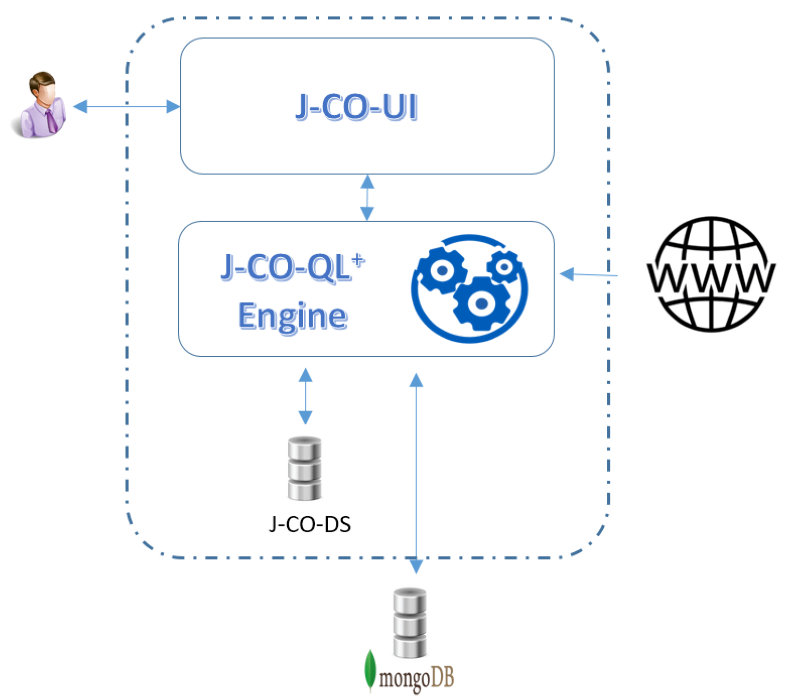
The paper is organized as follows. Section 2 presents relevant related work concerned with the paper. Section 3 provides a brief introduction to relevant concepts concerning fuzzy-set theory. Section 4 introduces the main features of the J-CO Framework. Section 5 precisely explains the addressed problem and introduces the methodology we follow, which relies on the concept of fuzzy relation. Section 6 presents and discusses the script written by means of J-CO-QL${}^{+}$, which practically applies the methodology presented in Section 5; each single instruction is explained, in order to illustrate how it behaves and its contribution within the script. Section 7 reports the results of an experimental evaluation, in which we evaluated effectiveness and, marginally, execution times. Finally, Section 8 draws the conclusions and possible future work.

2. Related Work

This paper embraces two different research lines: soft querying on databases in general and on JSON document stores in particular (Section 2.1), as well as the integration of data sets describing public places (Section 2.2).

2.1. Soft Querying on Databases

Providing data users with capabilities for flexibly querying databases is an old challenge. In particular, when selection conditions can rely on vague predicates, queries become “soft”, meaning that they are tolerant to thresholds (e.g., given a Boolean predicate price <= 30 to select cheap products, a product whose price is $30.45$ is not selected, while instead it could be of interest) and selected items could be ranked on the basis of their relevance to the selection condition. Fuzzy sets appeared as the formal framework to specify soft selection conditions [10]. Since relational-database technology dominated the panorama of database technology, many works were conducted to propose an extension of SQL (the standard query language for relational databases) towards soft querying based on fuzzy sets. Some popular proposals are SQLf [11,12] (for which we can mention an attempt to implement it [13]) and its extension named SQLf3 (which copes with constructs introduced in SQL3), as well as FQUERY for Access [14,15] (designed to operate on databases managed by Microsoft Access). Among all these proposals, SoftSQL [16,17,18] provided users with a statement to define non-trivial “linguistic predicates”, to be used in the extended SELECT statement to select table rows through linguistic predicates. The interested reader can find various surveys on the topic [19,20]; in particular, the work [21] is a very large handbook that summarizes all research work on this topic.

The advent of NoSQL (Not only SQL) databases [22], i.e., databases that do not rely on the classical relational model, has started a novel era in data management. In particular, the popularity obtained by the JSON (JavaScript Object Notation) format to represent any kind of complex data is facing the data engineer with the novel (with respect to relational databases) concept of “JSON document store”, i.e., a database which stores JSON documents in a native way. The most famous JSON document store is MongoDB [23], but many others are available (such as CouchDB [24], exploited within the block-chain platform called HyperLedger Fabric [25]). As a result, this novel scenario is revamping the topic of soft querying on databases, this time on NoSQL databases in general and on JSON document stores in particular.

An extension of MQL, the MongoDB query language, is proposed in [26]; in this extension, called “fMQL”, “fuzzy labels” can be used to query JSON documents, since they are equivalent to linguistic predicates; unfortunately, the work [26] does not provide any indication about how to define fuzzy labels. A further limitation of the proposal is that, for each single JSON document, only one membership degree is implicitly evaluated (in contrast, J-CO-QL${}^{+}$ allows for dealing with many membership degrees for each single document).

Finally, the work [27] proposes an approach for soft querying JSON documents: the corpus of JSON documents is preliminarily translated into fuzzy RDF triples [28]; then, the query is translated into fSPARQL [29], a fuzzy extension of SPARQL [30]. In our opinion, this approach is not suitable for processing JSON documents, because it does not work on the original documents, but on an alternative representation of them.

2.2. Integrating Data Sets Describing Public Places

The topic of aggregating information about public places coming from internet sources has been investigated in the last decade. Many different approaches have been followed.

For example, the work [31] adopts the DAS technique to integrate data about public places uniquely by exploiting string similarity on names, in particular by comparing the two strings without and with tokenization.

The work [32] compares different string-similarity metrics with various machine learning methods, to solve the problem of toponym matching. The results demonstrate that machine learning methods (in particular, classifiers) perform better than string-similarity metrics. Obviously, they cannot be applied from scratch, without preliminary labeling and training activities. Similarly, the work [33] exploits a neural network to perform “toponym matching”, i.e., pairing strings that represent the same location.

The work [34] addresses the problem of “geo-spatial data conflation” (the general name of the problem addressed in this paper) by adopting an entropy-based technique: the key idea is to use phonetic transcriptions, to compensate mistakes in writing names.

Another work that can be considered as related to this paper is [35], in which “semantic aligning” of heterogeneous geo-spatial data sets (GDs) is addressed. Specifically, it proposed an efficient similarity matching technique, which integrates various category systems simultaneously.

Finally, the closest work to this paper is [6]: this work could be considered the natural evolution of it. Specifically, a complex fuzzy relation is defined to perform public-place conflation in an on-line way. A comparison with a famous classification technique (i.e., “Random-Forest” classifiers) was performed, showing that the fuzzy approach is effective in a comparable way. Here, the definition of the fuzzy relation is improved to cope with not-cleaned names and addresses, as well as it is applied within the context of the J-CO Framework for the off-line integration of JSON data sets.

3. Basic Notions on Fuzzy Sets

In [36], Zadeh introduced the Fuzzy-Set Theory. It was rapidly clear that it had (and still has) an enormous potentiality to be successfully applied to many areas of computer science, such as decision making, control theory, expert systems, artificial intelligence, natural-language processing, and so on. Here, we report some basic concepts, which constitute the basis to understand the main contribution of this paper.

Definition 1.

Fuzzy Set. Consider a “universe set” U. A fuzzy set (or type-1 fuzzy set) A in U ($A\subseteq U$) is a mapping $A:U\to [0,1]$. The value $A\left(x\right)$ is referred to as the membership degree of the element x to the fuzzy set A. Alternatively, the notation ${\mu }_A\left(x\right)\in [0,1]$ can be used.

Clearly, given an item $x\in U$, if $A\left(x\right)=0$, this means that x does not belong at all to A; an intermediate value $0<A\left(x\right)<1$ means that x partially belongs to A (the greater the value, the higher its degree of membership); if $A\left(x\right)=1$, this means that the item x fully belongs to A.

Consequently, a fuzzy set is “empty” if and only if its membership function is identically zero for each $x\in U$.

Furthermore, given two fuzzy sets A in U and B in U, they are “equal” (denoted as $A=B$), if and only if $A\left(x\right)=B\left(x\right)$ (alternatively, ${\mu }_A\left(x\right)={\mu }_B\left(x\right)$) for all $x\in U$.

Operators on fuzzy sets can be easily defined, by extending the classical operators on traditional sets.

Definition 2.

Union, Intersection and Complement.Consider a universe U and two fuzzy sets A in U and B in U.

The union of two fuzzy sets A and B, denoted as $S=A\cup B$, generates a novel fuzzy set S whose membership function is $S\left(x\right)=max\left(A\right(x),B(x\left)\right)$, for each $x\in U$ (alternatively, ${\mu }_S\left(x\right)=max({\mu }_A\left(x\right),{\mu }_B\left(x\right))$).

The Intersection of two fuzzy sets A and B, denoted as $I=A\cap B$, generates a novel fuzzy set S whose membership function is $I\left(x\right)=min\left(A\right(x),B(x\left)\right)$, for each $x\in U$ (alternatively, ${\mu }_I\left(x\right)=min({\mu }_A\left(x\right),{\mu }_B\left(x\right))$).

The Complement of a fuzzy set A, denoted as $C=\overline{A}$, generates a novel fuzzy set C whose membership function is $C\left(x\right)=1-A\left(x\right)$, for each $x\in U$ (alternatively, ${\mu }_C\left(x\right)=1-{\mu }_A\left(x\right)$).

Classical logical operators are mapped onto operators on fuzzy sets: the OR operator is mapped onto the union; the AND operator is mapped onto the intersection; the NOT operator is mapped onto the complement.

Fuzzy sets are useful to represent vague concepts, which characterize many real-life application contexts. For example, if the universe is the set of people, we could think to divide them into “young” and “old”. However, is a person whose age is 40 actually young or old? He/she is a little bit young and a little bit old, neither fully young nor fully old.

Various other operators on fuzzy sets can be defined. In the following definition, we introduce the “weighted aggregation” operator.

Definition 3.

Weighted Aggregation. Given a universe U and two fuzzy sets A in U and B in U, the weighted aggregation operator $W=wa{g}_{\beta }(A,B)$ (with $\beta \in [0,1]$) generates a new fuzzy set W whose membership function is defined as $W\left(x\right)=\beta \times A\left(x\right)+(1-\beta )\times B\left(x\right)$ (alternatively, ${\mu }_W\left(x\right)=\beta \times {\mu }_A\left(x\right)+(1-\beta )\times {\mu }_B\left(x\right)$).

Example 1.

Through the membership degree, it is possible to denote partial membership of an item $x\in U$ to A; this way, vague linguistic concepts can be modeled. For example, given a public place p, its membership to the $PopularPlaces$ fuzzy set could be partial, denoting a place that is not so popular; thus, the membership degree measures its degree of popularity, for example on the basis of the number of likes obtained on social media.

Suppose that on the same universe of public places, we conceive the $CheapRestaurants$ fuzzy set, whose membership degree denotes the perception that a public place is cheap (this perception could be induced by analyzing menus published on social media).

We now illustrate how to aggregate the $PopularPlaces$ and the $CheapRestaurants$ fuzzy sets to obtain interesting places.

• If we are looking for “popularandcheap restaurants”, we could formulate the search as “$PopularPlaces$AND$CheapRestaurants$” (in terms of fuzzy sets, it is $I=PopularPlaces \cap CheapRestaurants$). Clearly, the lower membership degree determines the actual relevance of a place p.
• If we are looking for “popularorcheap restaurants”, we could formulate the search as “$PopularPlaces$OR$CheapRestaurants$” (in terms of fuzzy sets, it is $S=PopularPlaces \cup CheapRestaurants$). Clearly, the higher membership degree determines the actual relevance of a place p (a place could be not popular, but highly cheap).
• If we are looking for “popularand possiblycheap restaurants”, we could formulate the search as “70% $PopularPlaces$AND30% $CheapRestaurants$” (in terms of fuzzy sets, it is $W=wa{g}_{0.7}(PopularPlaces, CheapRestaurants)$). Clearly, the final membership degree is dominated by the degree of popularity, but a popular place that is also a cheap restaurant has a higher membership degree than a popular place that is not at all a cheap restaurant.

The three above-mentioned searches are examples of “soft queries”, where selection conditions are expressed in a vague way; the resulting membership degree denotes the “relevance” of an item to the soft query.

Furthermore, notice that when the names given to fuzzy sets linguistically characterize items in a proper way, these names can be used in soft conditions to linguistically express them.

Definition 4.

Fuzzy Relation. Consider two universes $U_1$ and $U_2$. A fuzzy relation R on $U_1$ and $U_2$, is defined as $R:U_1\times U_2\to [0,1]$. $R(x_1,x_2)\in [0,1]$, with $x_1\in U_1$ and $x_2\in U_2$, is the membership degree of the relation between $x_1$ and $x_2$; the meaning of the relation is linguistically expressed by the name of the relation.

Through the concept of fuzzy relation, it is possible to model the strength of a relation between two items $x_1\in U_1$ and $x_2\in U_2$. Nevertheless, notice that a fuzzy relation is a particular case of fuzzy set in the universe $U=U_1\times U_2$. Thus, we can reformulate the relation as $R:U\to [0,1]$, where $x=\langle x_1,x_2\rangle \in U$; consequently, we can write, in an equivalent way, either $R(x_1,x_2)$ or $R\left(\langle x_1,x_2\rangle \right)$.

In this paper, we work on the universe of JSON documents. So, given a document $d\in U$, the focus will be on the evaluation of its membership degrees to one or more fuzzy sets.

4. The J-CO Framework

The J-CO Framework is a suit of software tools able to process JSON data sets, in a way that is independent of the data source. In fact, it is able to obtain data sets both from JSON document stores (such as MongoDB) and from web sources. It is built around the J-CO-QL${}^{+}$ language and it contains various tools, as illustrated in Figure 1.

• The J-CO-QL${}^{+}$ Engine actually processes J-CO-QL${}^{+}$ queries. It obtains data to process from JSON document stores and from web sources; it is able to store results again into JSON document stores.
• J-CO-DS is a simplified JSON document store [37]: it is designed to provide users with the capability of storing large single JSON documents (usually, popular JSON document stores are not able to deal with very-large single JSON documents). J-CO-DS does not provide any internal computational capability, i.e., it does not provide a query language: in fact, it is part of the J-CO Framework, in which the component that provides computational capabilities is the J-CO-QL${}^{+}$ Engine.
• J-CO-UI is the user interface of the framework. It provides users with a graphical interface to interactively write J-CO-QL${}^{+}$ queries in a step-by-step way; users can also inspect intermediate results.

4.1. The Query Language

J-CO-QL${}^{+}$ is the current evolution of the original J-CO-QL (see [3,4,5]): as its predecessor, it is designed to provide high-level and declarative statements, which does not require programming skills to be used; by means of them, it is possible to specify complex procedures (scripts) that are able to retrieve, integrate, transform and save JSON data sets. With respect to its predecessor, J-CO-QL${}^{+}$ maintains the same approach, but revises syntax and semantics of statements, to improve their usability and effectiveness. Hereafter, we present its data model and its execution model.

4.1.1. Data Model

Here, we present the data model on which J-CO-QL${}^{+}$ relies.

• The basic item to process is a JSON document. A document is represented within a pair of braces “{” and “}”; it is a sequence of fields separated by commas.
  A field is a “name: value” pair, where “name” is the field name, while “value” is the value of the field; the name is always enclosed within double quotes (e.g., "name"); the value can be a number, a string (enclosed either within double quotes or single quotes), a Boolean value, a nested sub-document (enclosed within a pair of braces “{” and “}”) or an array (enclosed within square brackets “[” and “]”, whose items can be any kind of JSON value, separated by commas).
• J-CO-QL${}^{+}$ gives a special meaning to root-level fields whose name becomes with “~”; these names are compliant with JSON naming rules, but J-CO-QL${}^{+}$ considers some of them in a special way, as illustrated hereafter.

  -

  The root-level ~fuzzysets field is used to represent membership degrees of a d document to fuzzy sets. It works as a “key-value” map: given a field within ~fuzzysets, the field name is the name of the fuzzy set to which the membership degree has been evaluated; the value is a real number in the range $[0,1]$, which denotes the membership degree. This way, given a d document, it is possible to represent its membership to many fuzzy sets. 

  -

  The root-level ~geometry field represents geometries (also called “geo-tagging”) of spatial entities represented as JSON documents. In this paper, we do not make use of geometries (the interested reader can refer to [5]).

• A “collection” is an unordered multi-set of heterogeneous documents, i.e., it can contain multiple copies of the same document.

4.1.2. Execution Model

The execution model is the same presented in previous publications [5,7]. Hereafter, we briefly summarize it.

• A “query” $q=(i_1,i_2,\cdots ,i_n)$ is a sequence of instructions $i_j$, with $1\le j\le n$. A query is a “pipe of instructions”.
• Each instruction $i_j$ receives an input “query-process state” $s_{j-1}$ and generates a new query-process state $s_j$.
• A “query-process state” $s_j$ (with $0\le j\le n$) is a tuple $s_j=\langle tc,IR,DBS,FO,JSF\rangle$.

  -

  $tc$ is called “temporary collection”, since it is a collection of JSON documents that passes through the pipe of instructions, that contains temporary results of the query process. 

  -

  $IR$ is the “Intermediate-Results databaase”, i.e., a database that is exclusive for the query process, to store intermediate results to be used later. 

  -

  $DBS$ is the set of “database descriptors”, used to handle connections with external JSON document stores. 

  -

  $FO$ is the set of “Fuzzy Operators” defined within the query; they allows for evaluating membership degrees to fuzzy sets (see Section 6.2). 

  -

  $JSF$ is the set of user-defined “JavaScript Functions”; they are defined throughout the query to complete computational capabilities of the query language (see [38]).

• The initial query-process state is $s_0=\langle tc:\varnothing ,IR:\varnothing ,DBS:\varnothing ,FO:\varnothing ,JSF:\varnothing \rangle$. Each instruction possibly modifies one member of the query-process state.

5. Problem and Methodology

In this section, we discuss the premises from which the paper has originated and introduce the problem we addressed as a case study (Section 5.1). Then, we present the methodological framework, which this work relies on (Section 5.2).

5.1. Premises and Problem

In [6], a fuzzy method for the on-line aggregation of POIs (Points of Interest) is presented. The problem addressed in that paper can be summarized as follows: if a web application has to integrate descriptors of public places (or POIs) caught on the fly from external services, the decision whether two descriptors actually describe the same public place or not must be taken in real time: techniques that require off-line work cannot be used.

In [6], it was proved that the technique can obtain very high levels of accuracy, absolutely comparable with off-line techniques; consequently, here, we argue that the same technique could be effectively adopted to integrate two data sets describing public places, in an off-line way. In particular, the novel support for soft querying [7] provided by J-CO-QL${}^{+}$ (the query language of the J-CO Framework) has modified the scenario: in fact, the J-CO Framework is a stand-alone tool designed for manipulating and querying collections of JSON data sets. Consequently, it is straightforward to explore the possibility to exploit it for applying the fuzzy technique presented in [6] for integrating two collections of public-place descriptors coming from two different sources, by adopting a database approach (querying data by means of a query language) instead of hard coding the methodology with a programming language.

Hereafter, we present the problem. Then, Section 5.2 presents an improved formulation of the fuzzy technique presented in [6] that will be applied in J-CO-QL${}^{+}$ scripts (discussed in Section 6).

Problem 1.

Consider two collections of descriptors $D_1$ and $D_2$. A descriptor d (such that either $d\in D_1$ or $d\in D_2$) describes a public place; we assume that d is a tuple whose minimal shape is $d=\langle name,address,lat,lon\rangle$, where $d.name$ is the name of the public place, $d.address$ is the raw address (i.e., as it is provided by the data source, without any pre-processing or cleaning) of the public place, while $d.lat$ and $d.lon$ are, respectively, the latitude and longitude of the public place. Depending on the source, these fields could be missing (either null value or zero-length string).

Supposing that descriptors in $D_1$ and $D_2$ are related to the same municipality, we want to build the collection $SP=\{p_1,p_2,\cdots \}$ of pairs of descriptors $p_i:\langle d_{1,h},d_{2,k}\rangle$ (with $d_{1,h}\in D_1$ and $d_{2,k}\in D_2$) such that it is very likely that $d_{1,h}$ and $d_{2,k}$ actually describe the same public place.

5.2. Fuzzy Relation for Matching Public Places

The key contribution of [6] is a fuzzy relation called $MatchingPlaces$. Given two descriptors $d_1$ and $d_2$, it is written as $MatchingPlaces(d_1,d_2)$. Its membership degree denotes the possibility that $d_1$ and $d_2$ describe the same place. If we consider the universe $P=D_1\times D_2$ of pairs $p_i:\langle d_{1,h},d_{2,k}\rangle$, through the $MatchingPlaces$ fuzzy relation we want to build the fuzzy set $PRP$ in P of Possibly-Relevant Pairs for which the membership degree of $p_i$ is $PRP\left(p_i\right)>0$.

To actually decide whether descriptors in a $p_i$ pair actually describe the same public place, a minimum threshold $\alpha \in [0,1]$ is used to focus on Relevant Pairs $RP\subseteq PRP$, where $RP\left(p_i\right)\ge \alpha$.

However, given a descriptor $d_{1,h}\in D_1$, it could appear several times in $RP$, because there might be many relevant pairs in which it is involved. For each $d_{1,h}\in D_1$, the subset ${\overline{RP}}_{1,h}\subseteq RP$ is the set of pairs $p_i\in RP$ such that $p_1.d_1=d_{1,h}$; if ${\overline{RP}}_{1,h}$ is not empty, the pair $p_{1,h}\in {\overline{RP}}_{1,h}$ such that ${\overline{RP}}_{1,h}\left(p_{1,h}\right)\ge {\overline{RP}}_{1,h}\left(p_i\right)$, for all $p_i\in {\overline{RP}}_{1,h}$, appears in $SP$ (because the two paired descriptors are actually supposed to describe the same place).

In the remainder of this section, we introduce the complete formal framework.

5.2.1. Basic Functions and Relations

The $MatchingPlaces$ fuzzy relation is defined by means of some basic functions and fuzzy relations.

Given two pairs of coordinates, i.e., $la{t}_1,lo{n}_1$ and $la{t}_2,lo{n}_2$ (denoting latitude and longitude of two points on the earth globe), the $Distance$ function computes the “Geodesic Distance” [39] between the two points in km; it is denoted as $Distance(la{t}_1,lo{n}_1,la{t}_2,lo{n}_2)$. On this basis, it is possible to define the $Close$ membership function that, given a distance $dist$ (in km) determines whether the distance denotes that two points are close; it is denoted as $Close\left(dist\right)$; an example of a typical membership function for this concept (the same exploited in [6]) is depicted in Figure 2: notice that, on the basis of the geodesic distance between the two points, the membership degree is 1 when the distance is between 0 and 50 m; then, it linearly decreases from 50 up to 1000 m. In Section 6.2, we will define a more sophisticated membership function.

The $Close$ membership function can be used as the basis for defining the $ClosePlaces$ fuzzy relation: given two place descriptors $d_1$ and $d_2$, $ClosePlaces(d_1,d_2)=Close(Distance$$(d_1.lat,d_1.lon,d_2.lat,d_2.lon))$.

Given two strings $s_1$ and $s_2$, the $Similar$ fuzzy relation is denoted as $Similar(s_1,s_2)$. As a membership function, any string-similarity metric whose value is in the range $[0,1]$ could be used; in [6], the Jaro-Winkler similarity metric [40,41,42,43] was used; here, we still use it, but in a more sophisticated way (see Section 6.2).

Based on the $Similar$ relation, which is defined on the universe of strings, it is possible to define two derived relations that are defined on the universe of descriptor pairs $P=D_1\times D_2$.

The $SimilarAddress$ fuzzy relation denotes the extent to which the $address$ fields of the two descriptors are similar; it is defined as $SimilarAddress(d_1,d_2)=Similar(d_1.address,$$d_2.address)$.

The $SimilarName$ fuzzy relation denotes the extent to which the $name$ fields of the two descriptors are similar; it is defined as $SimilarName(d_1,d_2)=Similar(d_1.name,d_2.name)$.

5.2.2. The SameLocation Relation

The $MatchingPlaces$ relation is obtained by previously evaluating the $SameLocation$ fuzzy relation. It is denoted as $SameLocation(d_1,d_2)$. Its membership function changes, depending on the fact that fields concerning geographical aspects (i.e., address and coordinates) in $d_1$ and $d_2$ are missing or not. Hereafter, we provide three different definitions of the $SameLocation$ relation, one for each sub-case to deal with.

• Case A: missing address(es). If $d_1.address$ is missing, or $d_2.address$ is missing or both, but the two pairs of coordinates are available, only these latter ones can be used to evaluate the $SameLocation$ relation.
• Case B: missing coordinate(s). When one or more coordinates in $d_1$ and $d_2$ are missing, but both addresses $d_1.address$ and $d_2.address$ are available, only these latter ones can be used to evaluate the $SameLocation$ relation.
• Case C: addresses and coordinates are all available. When in $d_1$ and $d_2$ all geographical fields (i.e., address and coordinates) are available, they all contribute to the evaluation of the $SameLocation$ relation.

Once the three cases of interest have been identified, it is possible to define the $SameLocation$ relation.

Definition 5.

Case A. Given two descriptors $d_1$ and $d_2$, for which either $d_1.address$ or $d_2.address$ or both are missing, while the $lat$ and $lon$ fields are not null in both $d_1$ and $d_2$, the $SameLocation$ relation is defined as follows:

$SameLocation(d_1,d_2)=ClosePlaces(d_1,d_2)$

i.e., the membership degree of the $SameLocation$ relation coincides with the membership degree of the $ClosePlaces$ relation.

Definition 6.

Case B. Given two descriptors $d_1$ and $d_2$ for which at least one among $d_1.lat$, $d_1.lon$, $d_2.lat$ and $d_2.lon$ is null, while both $d_1.address$ and $d_2.address$ are available, the $SameLocation$ relation is defined as follows:

$SameLocation(d_1,d_2)=SimilarAddress(d_1,d_2)$

i.e., the membership degree of the $SameLocation$ relation coincides with the membership degree of the $SimilarAddress$ relation.

Definition 7.

Case C. Given two descriptors $d_1$ and $d_2$, for which all the fields $d_1.address$, $d_1.lat$, $d_1.lon$, $d_2.address$, $d_2.lat$ and $d_2.lon$ are available, the $SameLocation$ relation is defined as follows:

$SameLocation(d_1,d_2)=wa{g}_{{\beta }_{geo}}(SimilarAddress(d_1,d_2),ClosePlaces(d_1,d_2))$

i.e., the membership degree of the $SameLocation$ relation is the weighted aggregation of the $Similar$$Address$ relation and of the $ClosePlaces$ relation; ${\beta }_{geo}\in [0,1]$ is the weight of the first term (the similarity between addresses).

In Section 6.3, we use ${\beta }_{geo}=0.55$: this way, the similarity between addresses slightly prevails over closeness; indeed, if two addresses are very similar, their similarity contributes more than coordinates; this way, the effect of erroneous coordinates that give rise to high distances is mitigated.

5.2.3. Global MatchingPlaces Relation

At this point, we can define the global $MatchingPlaces$ relation.

Definition 8.

Given two descriptors $d_1$ and $d_2$, for which both fields $d_1.name$ and $d_2.name$ are available, and for which the $SameLocation$ relation is defined and $SameLocation(d_1,d_2)\ge {\alpha }_{geo}$ (with ${\alpha }_{geo}\in [0,1]$), the $MatchingPlaces$ relation is defined as follows:

$MatchingPlaces(d_1,d_2)=wa{g}_{{\beta }_{name}}(SimilarName(d_1,d_2),SameLocation(d_1,d_2))$

i.e., the membership degree of the $MatchingPlaces$ relation is obtained by aggregating the membership degrees of the $SimilarName$ relation and of the $SameLocation$ relation, by means of the weighted aggregator with weight ${\beta }_{name}$ for similarity of names.

In Section 6.4, we set ${\beta }_{name}=0.6$: this way, the similarity between names prevails over the membership degree of the $SameLocation$ relation. The rationale is the following: given two similar names, they contribute only for the $60\%$; the remaining $40\%$ is given by the geographical contribution. However, in order to avoid the two descriptors whose geographical contribution is not significant, the ${\alpha }_{geo}$ threshold is introduced: if the membership degree of the $SameLocation$ fuzzy relation is less than ${\alpha }_{geo}$, $d_1$ and $d_2$ are no longer considered eligible to be the same place: two places can have very similar names (even identical—imagine two restaurants of the same chain), but if there is the doubt that they are reasonably close, they could be a wrong pair. In Section 6.3, we set this threshold as ${\alpha }_{geo}=0.4$.

The membership degree of the $MatchingPlaces$ fuzzy relation is used to determine whether a pair actually belongs to the $RP$ set of relevant pairs, i.e., $RP\left(p_i\right)\ge \alpha$ means $MatchingPlaces$$(p_1.d_1,p_1.d_2)\ge \alpha$. In Section 6.4, we set this threshold as $\alpha =0.8$, because in our experiments (see Section 7.1), we found this is the threshold that gives the best effectiveness.

6. Presenting the Script

In this section, we provide the technical contribution of the paper. Specifically, we demonstrate how the current version of J-CO-QL${}^{+}$ is able to perform the soft integration of two collections containing JSON documents that describe public places, obtained from two different data sources.

6.1. Data Set

A MongoDB database called ijgiDb contains two collections of JSON documents: the first one is called FacebookDescriptors and its documents are descriptors of pages that present public places mostly located in the area of Manchester (UK); the second collection is called GoogleDescriptors and its documents are descriptors of places mostly located in the area of Manchester (UK) as well, obtained from Google Places. The FacebookDescriptors collection contains 5738 documents, while the GoogleDesciptors collection contains 5214 documents. 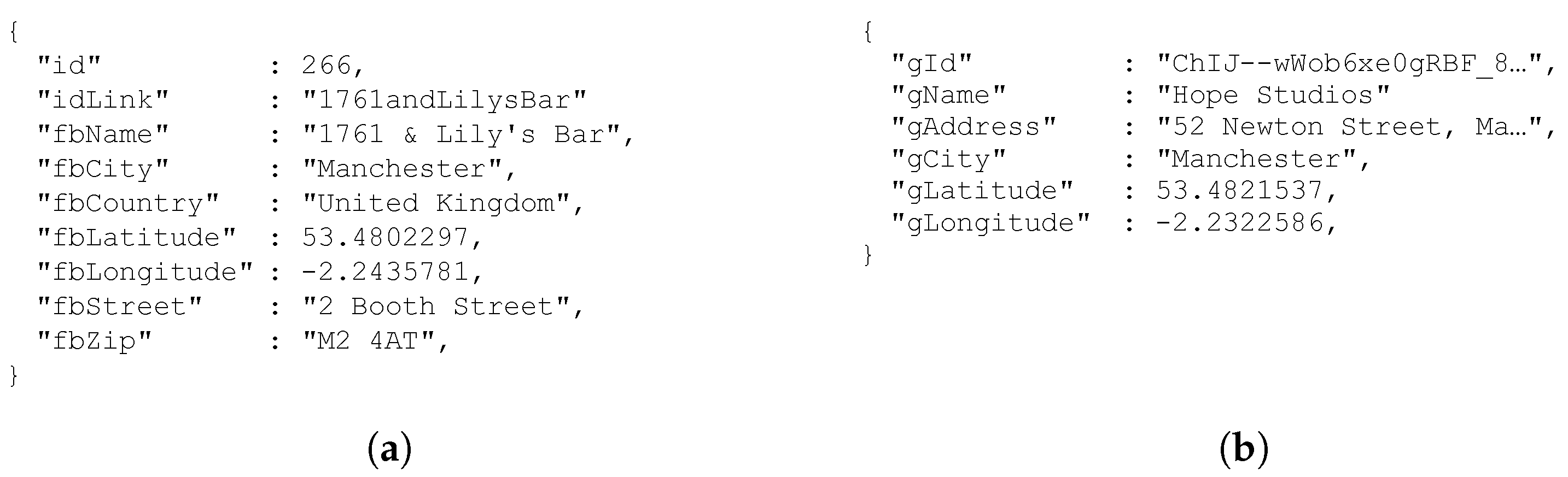Figure 3a shows a sample document in the FacebookDescriptors collection, while Figure 3b reports a sample document in the GoogleDescriptors collection. The reader can notice that Facebook descriptors clearly distinguish the address (in the fbStreet field) from the city name (in the fbCity field) from the ZIP code (in the fbZip field). In contrast, within a Google Places descriptor, the content of the gAddress field is less clean, because it contains the city name too. This also demonstrates that we are working on names and addresses as they are provided by Facebook and Google Places, without any pre-processing or cleaning (in [6], addresses were cleaned from numbers and urban designations, such as “street”). Consequently, here, we are addressing a less favorable situation.

6.2. Defining Fuzzy Operators

We start presenting the J-CO-QL${}^{+}$ script. The first part of the script is reported in Listing 1.

The key concept provided by J-CO-QL${}^{+}$ to evaluate membership degrees of JSON documents is the concept of “fuzzy operator”. Such an operator is called within soft conditions: given some actual parameters (expressions based on document fields), the operator returns a membership degree. This degree will be used to evaluate the overall membership degree of a document to a specific fuzzy set.

Listing 1. J-CO-QL${}^{+}$ script: fuzzy operators.

Listing 1. J-CO-QL${}^{+}$ script: fuzzy operators.

6.2.1. The Close Fuzzy Operator

The instruction on line 1 of the J-CO-QL${}^{+}$ script in Listing 1 defines the Close fuzzy operator: it evaluates the degree of closeness of two places, on the basis of the distance between them. Hereafter, we describe the instruction in details.

• The PARAMETERS clause defines the formal parameters of the operator. Specifically, only the distance parameter is defined.
• The PRECONDITION clause defines a condition on the parameters: if the condition is not satisfied, the evaluation of the fuzzy operator stops and an error signal is raised. Specifically, the precondition says that the distance must be no less than 0.
• The EVALUATE clause specifies a mathematical expression on the parameters, whose value is used as x-axis coordinate against the membership function defined by the subsequent POLYLINE clause. In the Close fuzzy operator, the expression simply takes the value of the distance parameter.
• The POLYLINE clause specifies the membership function actually used to compute the membership value. The function is defined as a polyline, by a sequence of pairs $(x_i,y_i)$, where $x_i$ can be any real value, while $y_i\in [0,1]$; given two consecutive points $(x_i,y_i)$ and $(x_{i+1},y_{i+1})$, it must be $x_i<x_{i+1}$. Each pair of consecutive points defines a segment. Given an x value, if it is between $x_1$ and $x_n$ (in the case of n points), the corresponding y value is considered as a membership degree; if $x<x_1$, the membership degree is $y_1$; if $x>x_n$, the membership degree is  $y_n$.

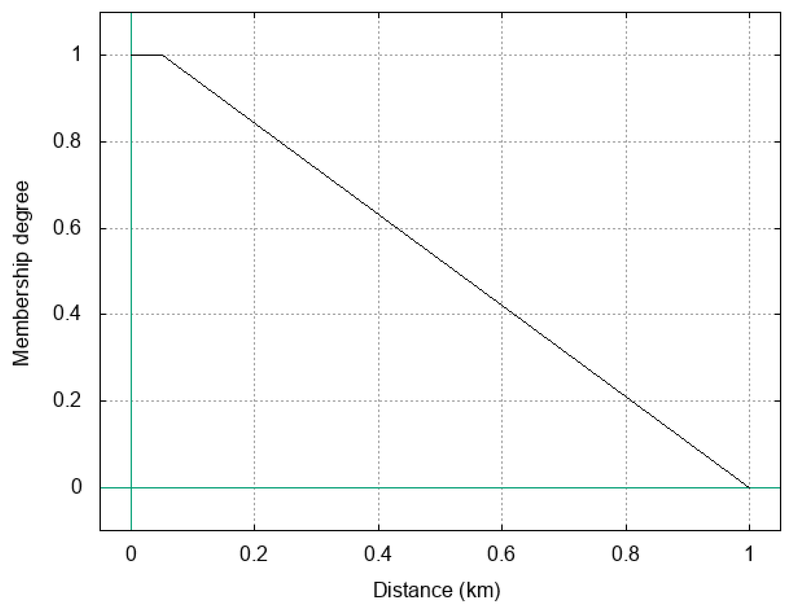
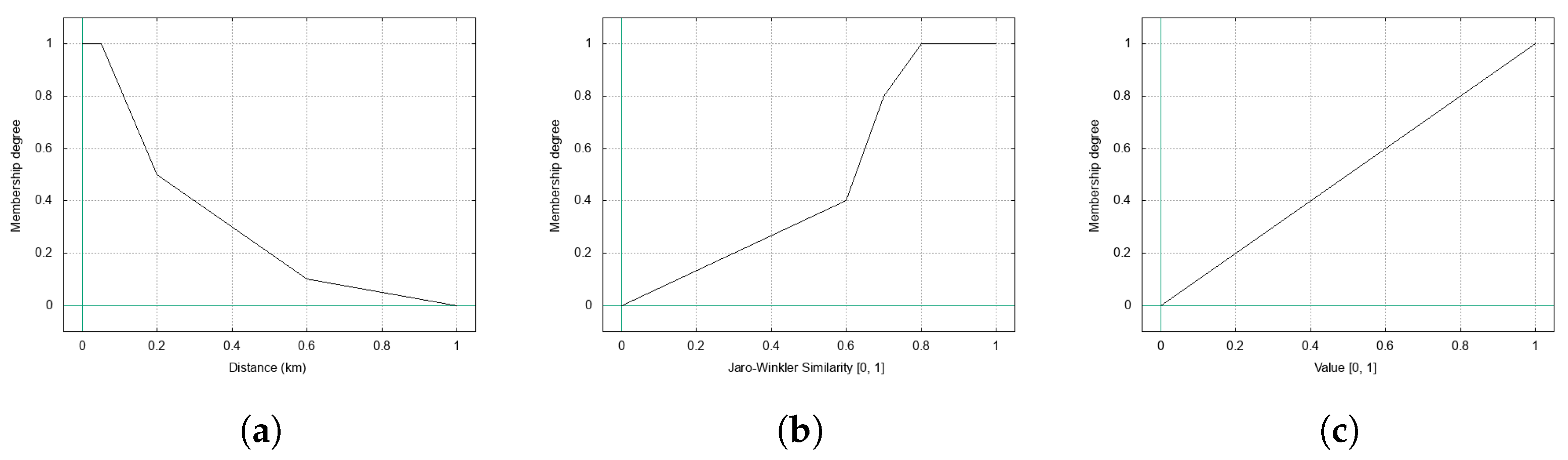
Figure 4a reports the polyline defined for the Close fuzzy operator. Notice that it is not the same defined in [6] (reported in Figure 2): in fact, we opted for a function that immediately penalizes distances that are between 50 m and 600 m, because two places in the same neighborhood are not perceived as very close when their distance becomes greater than 100 m.

6.2.2. The Similar Fuzzy Operator

The instruction on line 2 of the J-CO-QL${}^{+}$ script in Listing 1 creates the Similar fuzzy operator. Its goal is to evaluate a membership degree on the basis of the similarity degree of two strings. The operator is described in detail hereafter.

• The operator receives two parameters, called st1 and st2; they are the two strings to compare.
• No precondition is specified: in the case of empty or null strings, the operator returns 0 as membership degree, because the similarity degree is 0.
• The EVALUATE clause calls the built-in (i.e., provided by J-CO-QL${}^{+}$) function named JARO_WINKLER_SIMILARITY, to obtain the similarity degree of the two strings. The similarity degree is a value in the range $[0,1]$. In the case of null or zero-length strings, the returned similarity degree is 0.
• The POLYLINE clause defines the membership function depicted in Figure 4b. Notice that it penalizes similarity degrees that are less than $0.7$, while membership degrees that are greater than $0.8$ are rewarded: this is due to the sometimes bizarre behavior of the Jaro-Winkler similarity, that returns high similarity degrees even when strings only shares some characters, but are not actually similar; furthermore, for strings such as “The Gray Horse” and “GrayHorse”, the similarity degree is around $0.7$, although they clearly have to be considered very similar. With this shape, we try to compensate the behavior of the Jaro-Winkler similarity, so as to deal with raw addresses and names (i.e., not cleaned from articles, numbers, punctuation, and so on).

6.2.3. The WeightedAggregationBeta Fuzzy Operator

The instruction on line 3 of the J-CO-QL${}^{+}$ script in Listing 1 defines the third fuzzy operator. This is called WeightedAggregationBeta and its goal is to perform the “weighted aggregation” $wa{g}_{\beta }$ (see Definition 3). In fact, J-CO-QL${}^{+}$ does not provide such an operator in its language; through the WeightedAggregationBeta fuzzy operator, we show how to introduce novel fuzzy concepts. The fuzzy operator is described in detail hereafter.

• The operator receives three parameters: f1 and f2 are the two values in the range $[0,1]$ to aggregate, while beta is the aggregation weight (in the range $[0,1]$ too) of f1 with respect to f2.
• The PRECONDITION clause ensures that the actual values of the three parameters are in the range $[0,1]$ (notice the IN_RANGE predicate).
• The EVALUATE clause actually performs the weighted aggregation.
• The POLYLINE clause defines a very simple membership function, which is reported in Figure 4c: it is a straight segment from the point $(0,0)$ to the point $(1,1)$; this way, the value computed by the EVALUATE clause is returned, as it is, as membership degree.

6.3. Retrieving and Pairing Descriptors

Once the three fuzzy operators are defined, it is time to start working on the data set. This is conducted by the second part of the J-CO-QL${}^{+}$ script, which is reported in Listing 2.

Listing 2. J-CO-QL${}^{+}$ script: retrieving and joining collections.

Listing 2. J-CO-QL${}^{+}$ script: retrieving and joining collections.

The instruction on line 4 connects the query process to the database. After this instruction, it will be possible to access the ijgiDb database to retrieve and store collections.

The JOIN OF COLLECTIONS instruction on line 5 retrieves the two source collections (called FacebookDescriptors and GoogleDescriptors) and creates all possible pairs of documents contained in the two collections. Then, the subsequent CASE clause evaluates a pool of conditions on these pairs to possibly evaluate fuzzy sets on the actually-interesting pairs and discards the others. The instruction is explained in detail hereafter.

• The instruction retrieves the FacebookDescriptors collection from the ijgiDb database and aliases it as f; similarly, it retrieves the GoogleDescriptors collection from the same database and aliases it as g.
  For each f document from the f collection and for each g document from the g collection, a new d document is created. This document contains two fields: the first one is called f and its value is the source f document; the second one is called g and its value is the source g document. The d document is further processed by the subsequent CASE clause.
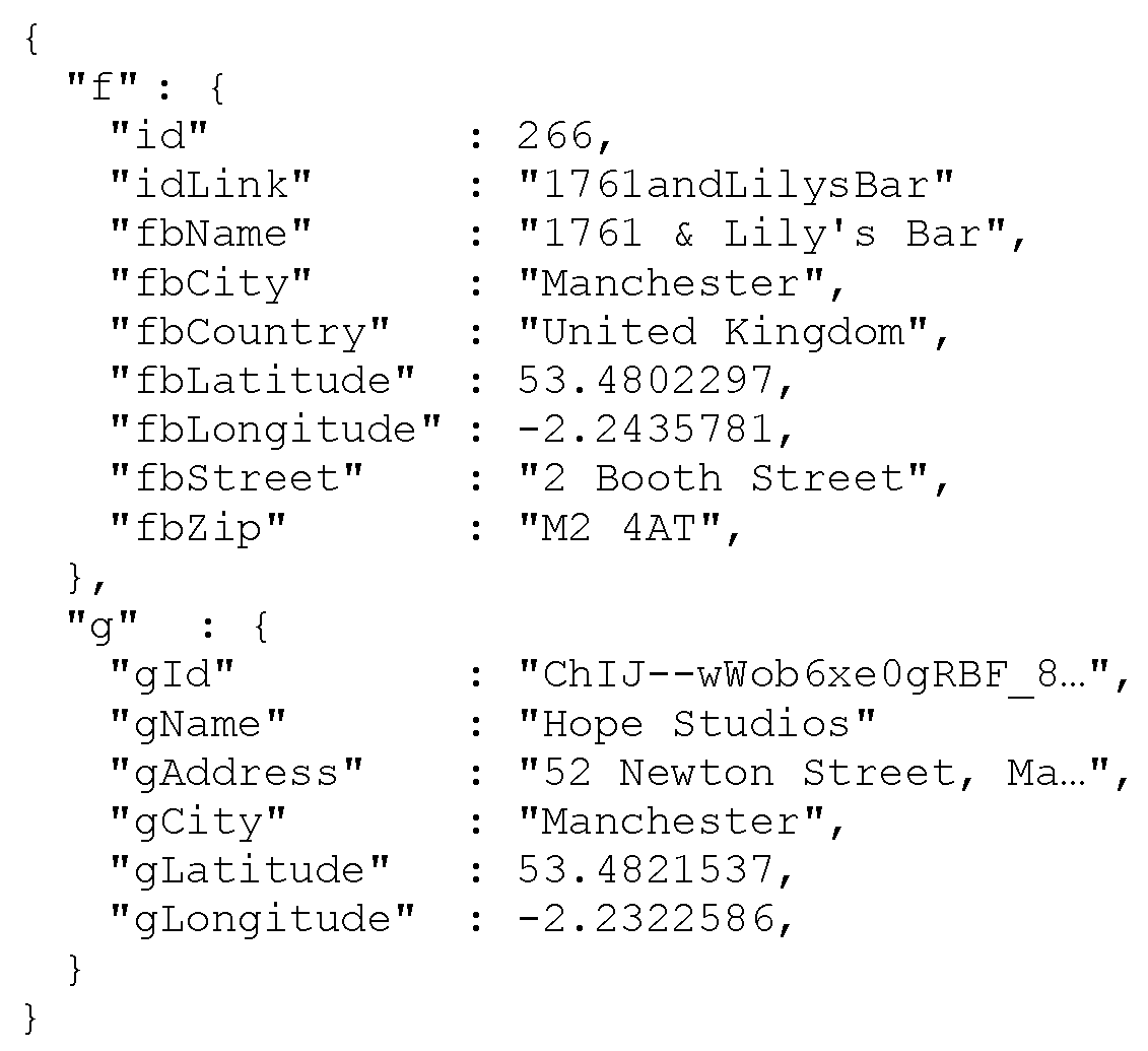
  Figure 5 reports an example of d document, which is obtained by joining the two sample documents reported in Figure 3; notice the names of the root-level fields.
• The CASE clause evaluates a pool of selection conditions expressed within a WHERE clause; if a d document is selected by a condition, it is processed according to the subsequent sub-clauses. Many WHERE branches are possible: a d document is processed by the branch associated with the first WHERE condition that it satisfies; if no condition is satisfied, d is discarded (it will not appear in the output temporary collection).
  Specifically, the CASE clause in the instruction on line 5 in Listing 2 contains three WHERE branches: each of them deals with one of the three situations considered for defining the $SameLocation$ relation by Definitions 5–7. Hereafter, we separately discuss the behavior of the three branches.

  -

  The first WHERE branch deals with the case A of the $SameLocation$ fuzzy relation, defined in Definition 5. The condition is true if either the value for the fbStreet field is missing or the value for the gAddress field is missing or both are missing, and all coordinates are available. If a d document meets the condition, the GENERATE block further processes d through the CHECK FOR clause, whose goal is to evaluate the membership degrees of d to fuzzy sets.

  Specifically, two FUZZY SET branches are present: the former evaluates the ClosePlaces fuzzy set, the latter evaluates the SameLocation fuzzy set.

  The membership degree to the ClosePlaces fuzzy set is obtained by the associated USING clause: this is a “soft condition”, in which fuzzy operators (such as those defined in Section 6.2) and fuzzy-set names can be composed by the usual (fuzzy) logical operators AND, OR and NOT; the resulting membership degree is the membership degree to the evaluated fuzzy set. If this is the first membership degree evaluated for d, then d does not have the special ~fuzzysets field: in this case, the field is added and within it only one single field is present, having the same name of the evaluated fuzzy set, whose value is the computed membership degree. In contrast, if the ~fuzzysets field is already present, it is extended with one extra internal field, describing the membership degree to the new evaluated fuzzy set.

  Specifically, the first branch evaluates the membership degree to the ClosePlaces fuzzy set, by means of the Close fuzzy operator (see Listing 1), which is called passing the geodesic distance computed by the GEODESIC_DISTANCE built-in function.

  The second FUZZY SET branch evaluates the membership degree to the SameLocation fuzzy set, by assuming that it coincides with the ClosePlaces fuzzy set (see Definition 5). Finally, the ALPHACUT clause discards the d document from the output temporary collection if its membership degree to the SameLocation fuzzy set is less than $0.4$; remember that this is the ${\alpha }_{geo}$ threshold mentioned within Definition 8. 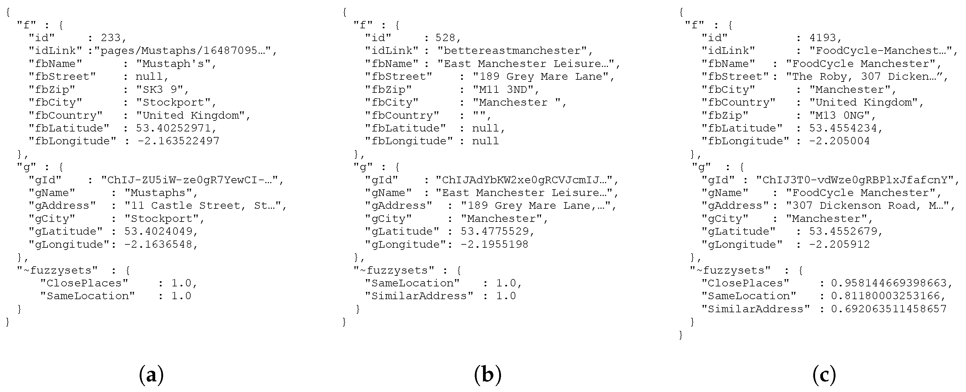Figure 6a reports a sample document generated by the first WHERE branch; notice the presence of the ~fuzzysets field and its inner fields.  

  -

  The second WHERE branch deals with case B of the $SameLocation$ relation (see Definition 6), i.e., at least one coordinate is null but both addresses are present.

  In this case (see Definition 6), the membership degree to the SimilarAddress fuzzy set is evaluated by means of the Similar fuzzy operator, which evaluates the fuzzy similarity relation between two strings (in this case, the two addresses).

  Then, as defined by Definition 6, the second FUZZY SET branch tells that the SameLocation fuzzy set coincides with the SimilarAddress fuzzy set. Again, the ALPHACUT clause puts the d document into the output temporary collection if the membership degree to the SameLocation fuzzy set is no less than $0.4$ (the ${\alpha }_{geo}$ threshold in Definition 8). Figure 6b shows a sample document generated by the second WHERE branch.  

  -

  The third WHERE branch deals with case C of the $SameLocation$ fuzzy relation (see Definition 7), i.e., both all addresses and all coordinates are available. Consequently, the membership degrees to three different fuzzy sets are evaluated: the first one is the SimilarAddress fuzzy set, by means of the Similar fuzzy operator applied to addresses; the second one is the ClosePlaces fuzzy set, by means of the Close fuzzy operator applied to the geodesic distance between the two points.

  The third FUZZY SET branch evaluates the membership degree to the fuzzy set named SameLocation: according to Definition 7, it is obtained by calling the WeightedAggregationBeta fuzzy operator, whose goal is to perform the weighted aggregation: it receives the two values (in the range $[0,1]$) to aggregate and the $\beta$ weight.

  The USING soft condition calls the WeightedAggregationBeta fuzzy operator, passing the membership values to the SimilarAddress fuzzy set and to the ClosePlaces fuzzy set, which are obtained by means of the MEMBERSHIP_OF built-in function (that extracts the membership degree from within the ~fuzzysets field). The third parameter is the constant value $0.55$: thisis the ${\beta }_{geo}$ weight presented and discussed in Definition 7. The ALPHACUT clause discards the evaluated document if its membership degree to the SameLocation fuzzy set is less than $0.4$ (the ${\alpha }_{geo}$ threshold mentioned in Definition 8).

  Figure 6c reports a sample document generated by the third branch; notice that the ~fuzzysets field has three inner fields.

The temporary collection produced by the instruction on line 5 of Listing 2 contains heterogeneous documents, as far as the structure of the ~fuzzysets field is concerned, but all have the inner SameLocation field, denoting the membership degree to the SameLocation fuzzy set; it will be used in the next instruction, to evaluate the membership degree to the MatchingPlaces fuzzy set.

Furthermore, notice that SameLocation, ClosePlaces and SimilarAddresses are called “fuzzy sets”, while they were defined in Section 5 as “fuzzy relations”: this is not a mistake, but the consequence of the fact that JSON documents represent pairs of descriptors; consequently, fuzzy relation on pairs are translated into fuzzy sets on JSON documents.

6.4. Relevant Pairs

All documents contained in the temporary collection produced by the instruction on line 5 (Listing 2) have the membership degree to the SameLocation fuzzy set no less than ${\alpha }_{geo}=0.4$, as required by Definition 8. The FILTER instruction on line 6 in Listing 3 actually evaluates the membership degree to the MatchingPlaces fuzzy set, which corresponds to the $MatchingPlces$ relation defined in Definition 8. The FILTER instruction on line 6 is described in detail hereafter.

• The FILTER statement takes the temporary collection as input and generates a new temporary collection by applying a CASE clause. The behavior of this clause is the same as in the JOIN OF COLLECTIONS statement.
• On line 6, only one WHERE branch is present: if a document does not meet the selection condition, it is discarded from the output temporary collection.
  Specifically, the selection condition selects those documents having both the names in the two paired descriptors, so as to evaluate the membership degree to the SimilarName fuzzy set.
• The first FUZZY SET branch in the CHECK FOR clause evaluates the membership degree to the SimilarName fuzzy set; again, in the USING soft condition, the Similar fuzzy operator (see Listing 1) is called, this time passing names (instead of addresses).
• The second FUZZY SET branch can finally evaluate the membership degree to the MatchingPlaces fuzzy set, corresponding to the $MatchingPlaces$ fuzzy relation defined by Definition 8. Remember that the fuzzy relations named $SameLocation$ and $SimilarName$ are aggregated by means of the weighted aggregation operator. In Listing 1, we defined the WeightedAggregationBeta fuzzy operator, which here is used to aggregate the SimilarName fuzzy set and the SameLocation fuzzy set; the SimilarName fuzzy set weights for the $60\%$ of the final membership degree (this is the ${\beta }_{name}$ weight mentioned in Definition 8), so that similarity between names moderately prevails over geographical similarity (whose goal is to cofirm that two places having similar or identical names are actually the same place). The resulting membership degree becomes the membership degree to the MatchingPlaces fuzzy set.
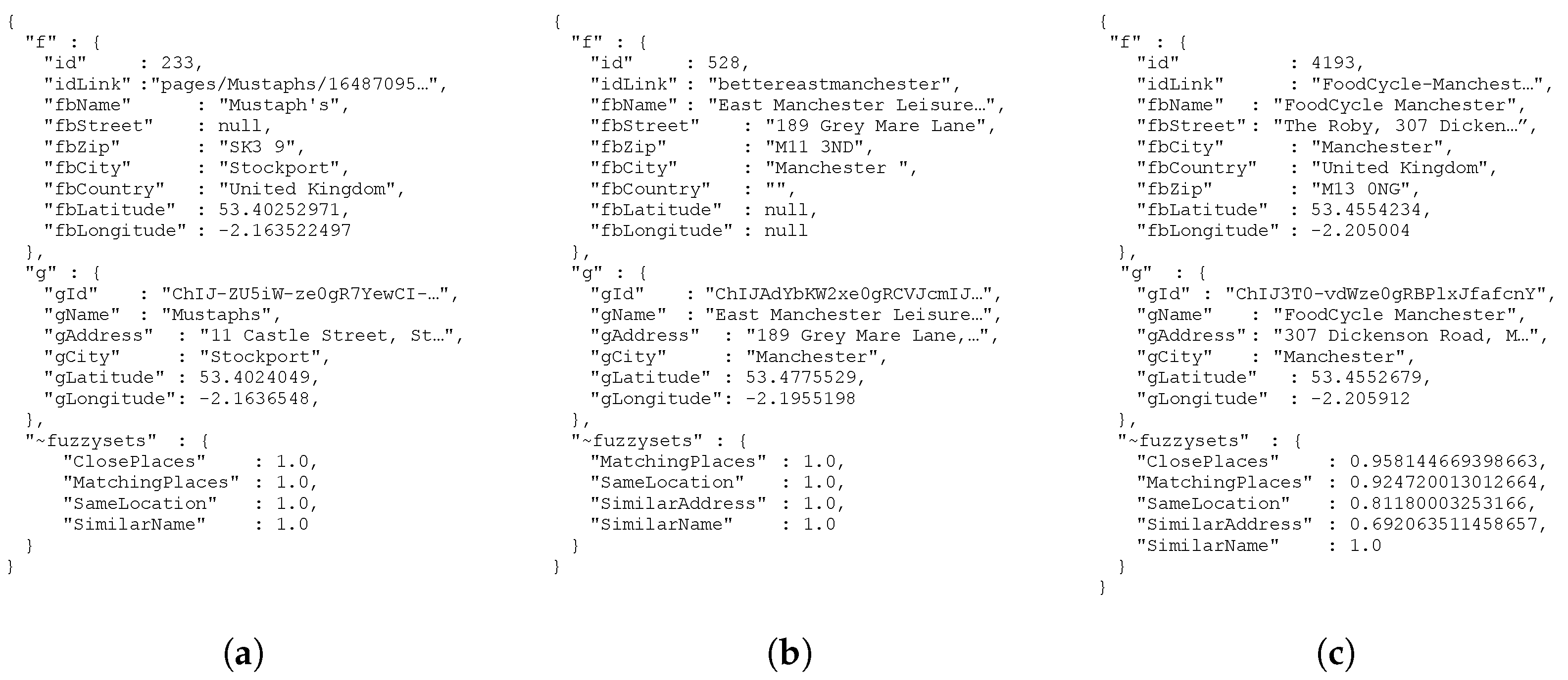
  The three sample documents reported in Figure 6 become as reported in Figure 7; notice the presence of the MatchingPlaces inner field within the ~fuzzysets field.
• At this point, only relevant pairs must be kept, i.e., those pairs whose membership degree to the MatchingPlaces fuzzy set is no less than $\alpha =0.8$. The ALPHACUT clause does that.
• The final BUILD section (which is optional, this is why it was not present in the JOIN OF COLLECTIONS instruction on line 5 in Listing 2) restructures all survived documents.
  Specifically, a novel rank field is added, whose value is the membership degree to the MatchingPlaces fuzzy set. This field is necessary, because the subsequent DEFUZZIFY option discards the ~fuzzysets field (as a consequence, documents are “defuzzified”).
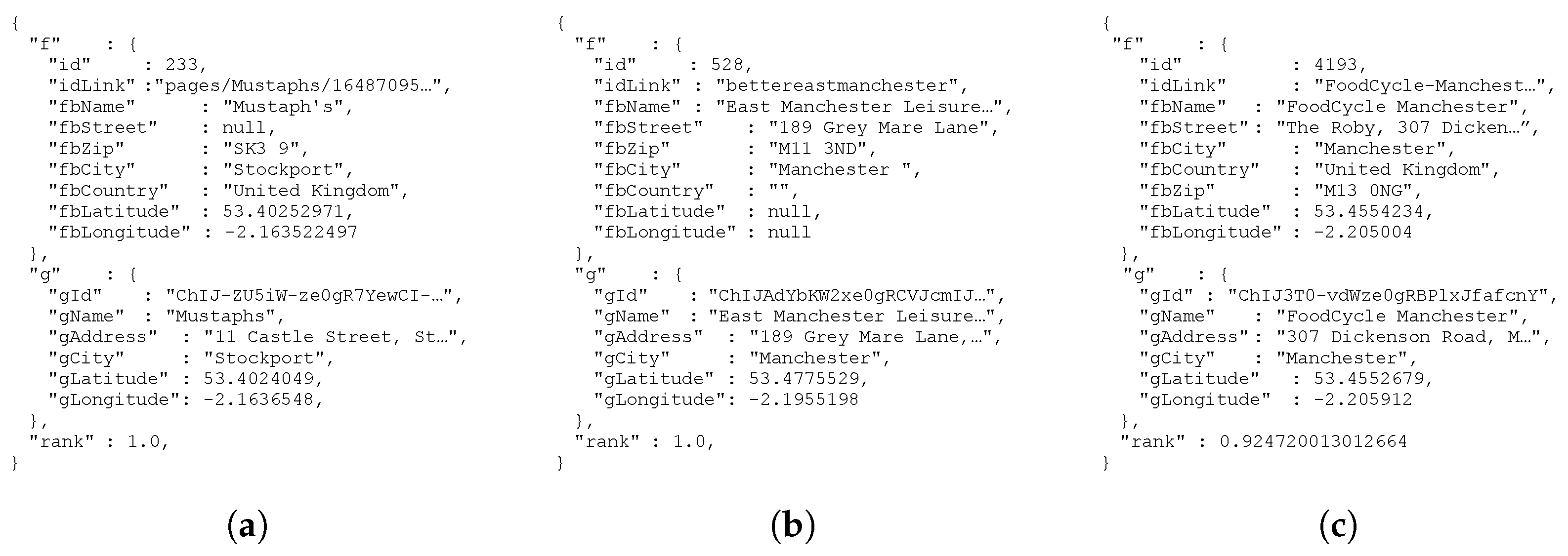
  Figure 8 reports the final state of the three sample documents reported in Figure 7. Notice the presence of the rank field, whose value is the membership degree of the MatchingPlaces fuzzy set.

Listing 3. J-CO-QL${}^{+}$ script: matching places.

Listing 3. J-CO-QL${}^{+}$ script: matching places.

The instruction on line 7 in Listing 3 saves the temporary collection into the ijgiDb database, with name RelevantPairs. Its documents contain the most promising pairs of descriptors (remember the $RP$ set mentioned in Section 5.2), but it could happen that, e.g., the same Google Places descriptor is associated with more than one Facebook descriptor. Clearly, it is the case to choose the pair having the highest rank (i.e., building the final $SP$ set mentioned in Section 5.2). This is discussed in Section 6.5.

6.5. Choosing the Best Pairs

The last part of the J-CO-QL${}^{+}$ script is reported in Listing 4. It actually chooses the best pairs that involves each single Google Places descriptor obtained by line 6 in Listing 3. Indeed, the original J-CO-QL language (from which J-CO-QL${}^{+}$ derives) was designed to cope with this kind of task too (see [3,4]). Hereafter, we briefly describe this last part of the script.

• The GET COLLECTION instruction on line 8 again obtains the RelevantPairs collection from the database, again making it the temporary collection.
• The GROUP instruction on line 9 groups documents in the temporary collection, on the basis of the gId field, which is the identifier of Google Places descriptors. For each group, a novel document is generated into the output collection, such that it has the gId field and an array called gGroup, in which all grouped documents are reported. This array is sorted in reverse order of value of the rank field within grouped documents. 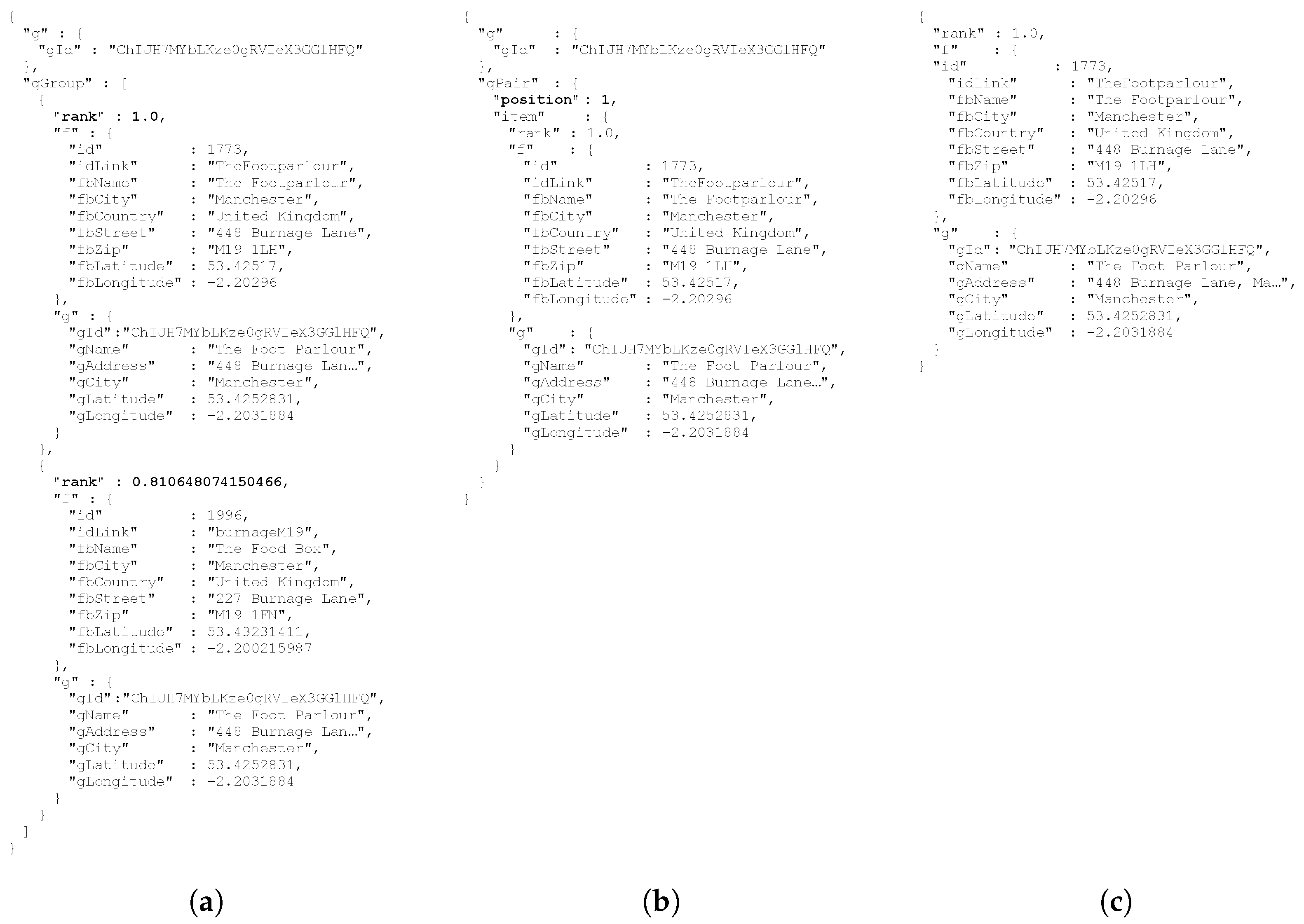Figure 9a reports an example of the grouped document.
• The EXPAND instruction on line 10 unnests again all grouped documents. For each output document, the gPair field is added to the global ones (apart from the expanded array); this new field contains two inner fields: the item field contains the unnested document; the position field denotes the position occupied by the unnested item in the gGroup array.
  As a result, the temporary collection generated by line 10 contains as many documents in the RankedPairs collection, but now they are tagged with the relative order for Google Places descriptors on the basis of the rank field. Figure 9b reports an example of an unnested document.
• The FILTER instruction on line 11 actually selects only documents that previously occupied the first position in their group (based on the reverse order of rank, they are the ones with the highest rank). The BUILD section builds the same structure again, as in the RelevantPairs collection. Figure 9c reports an example of resulting document.
• Finally (on line 12) the last temporary collection is saved into the ijgiDb database with name SamePlaces, which is the desired output of the process.

Listing 4. J-CO-QL${}^{+}$ script: Selecting the best pairs.

Listing 4. J-CO-QL${}^{+}$ script: Selecting the best pairs.

7. Experimental Evaluation

In this section, we report a brief evaluation of the results that can be obtained by the J-CO-QL${}^{+}$ script. We exploited the same data set adopted in [6], related with the city of Manchester (UK). Remember, from Section 6.1, that the FacebookDescriptors collection contains 5738 descriptors, while the GoogleDescriptors collection contains 5214 descriptors. Both collections contain descriptors about a variety of different public places, such as restaurants, pubs, hairdressers, universities, parks and so on.

7.1. Effectiveness

In order to evaluate the effectiveness of the method, we performed a sensitivity analysis by varying the value of the $\alpha$ threshold from $0.5$ to $0.99$.

We used the same test set again, which was used in the work [6]: it contained a total of 400 pairs, selected among the $5738\times 5214$ total pairs, evaluated by a human as $Good$ or $Bad$. We randomly selected 300 pairs from the starting 400 pairs, and from each pair we extracted the related 300 Google Places descriptors and 300 Facebook descriptors; among all possible pairs, 103 pairs were labeled as $Good$ pairs (and obviously the remaining 197 were labeled as $Bad$).

Then, we run the script on these two reduced collections of descriptors.

Table 1. Sensitivity analysis.

Alpha Cut	Relevant Pairs	Same Places	TP	TN	FP	FN	Precision	Recall	Accuracy
0.50	253	163	103	137	60	0	0.632	1.000	0.800
0.55	178	139	103	161	36	0	0.741	1.000	0.880
0.60	140	124	103	176	21	0	0.831	1.000	0.930
0.65	119	112	103	188	9	0	0.920	1.000	0.970
0.70	110	108	101	190	7	2	0.935	0.981	0.970
0.75	109	107	101	191	6	2	0.944	0.981	0.973
0.80	106	105	101	193	4	2	0.962	0.981	0.980
0.85	98	97	97	197	0	6	1.000	0.942	0.980
0.90	90	90	90	197	0	13	1.000	0.874	0.957
0.95	80	80	80	197	0	23	1.000	0.777	0.923
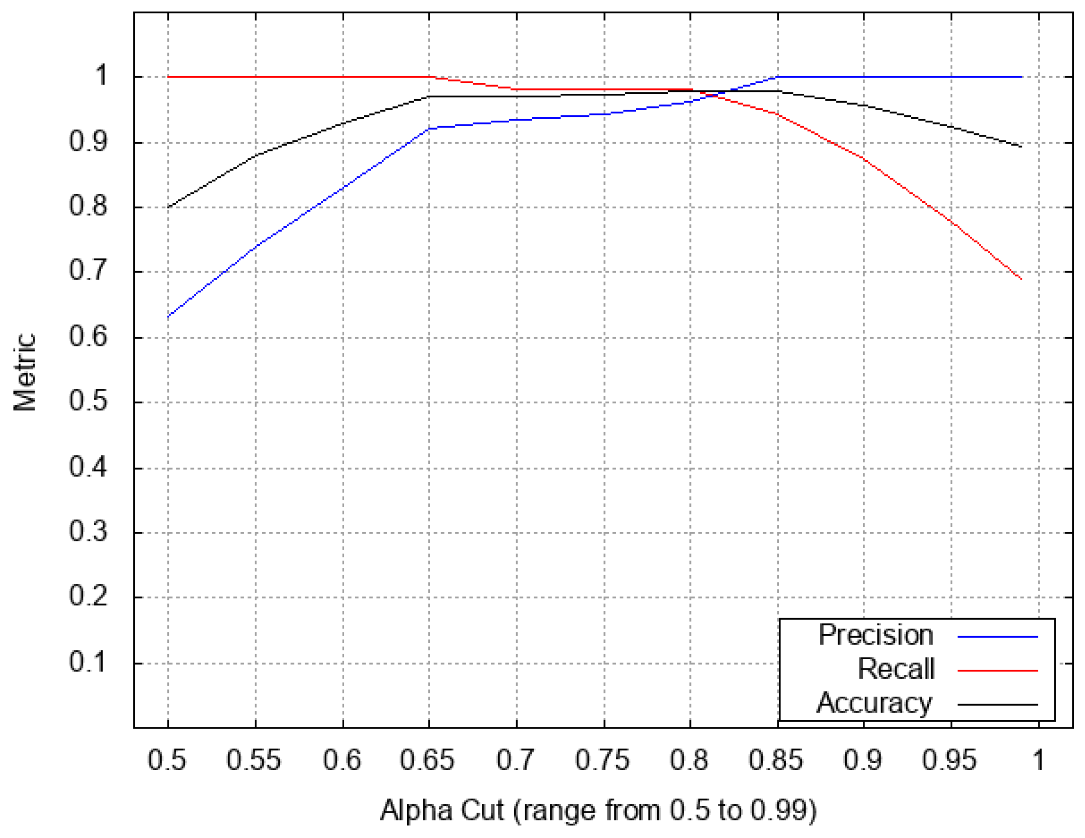
0.99	71	71	71	197	0	32	1.000	0.689	0.893

reports the results of our experiments. Specifically, the first colum reports the single values for the alpha-cut $\alpha$; the second and third columns report the number of relevant pairs saved by line 7 of the J-CO-QL${}^{+}$ script (Listing 3) into the RelevantPairs collection and the number of pairs generated by line 12 of the script (Listing 4) and saved into the SamePlaces collection, respectively. The, columns from 4 to 7 reports the number $TP$ of true positive pairs, the number $TN$ of negative pairs, the number $FP$ of false positive pairs and the number $FN$ of false negative pairs, respectively. Finally, the last three columns reports “Precision” (defined as $TP/(TP+FP)$), “Recall” (defined as $TP/(TP+FN)$) and “Accuracy” (defined as $(TP+TN)/(TP+TN+FP+FN)$), respectively. These three latter values are depicted in Figure 10: the x-axis reports the values of the alpha-cut $\alpha$ parameter; precision is depicted by the blue line, recall is depicted by the red line and accuracy is depicted by the black line.

Analyzing Table 1 and Figure 10, it is possible to see that the best combination of values for precision, recall and accuracy were obtained for $\alpha =0.8$: precision is $0.962$, recall is $0.981$ and accuracy is $0.980$. Indeed, this value for $\alpha$ appears to be the best compromise between the need to keep as many pairs as possible and the fact that those pairs actually describe the same place, even though names, addresses and coordinates are different. The reader can further notice that higher values of $\alpha$ give rise to a precision of 1 with poor recall, while lower values for $\alpha$ give rise to a recall of 1 with poor precision. To conclude this analysis, notice that with $\alpha =0.85$, the accuracy is the same as the one obtained for $\alpha =0.8$; it could be considered as a valid alternative choice, with better precision but low recall.

Thus, we can state that the novel formulation for the $MatchingPklaces$ relation and the complex membership functions adopted for the Similar fuzzy operator and for the Close fuzzy operator are effective, provided that $\alpha =0.8$.

We can consider the results reported in [6] as a baseline for further evaluating the effectiveness of the novel formulation of the technique.

Remember that the version presented in [6] (for on-line aggregation) performed pre-processing tasks on names and addresses, so as to clean them from urban designations and numbers. In contrast, the present version does not. The main reason is that such a kind of pre-processing and cleaning is not easy to do within J-CO-QL${}^{+}$ scripts; however, the flexibility of the CREATE FUZZY OPERATOR statement as far as the possibility to define complex shapes for membership functions seems to be effective. Consequently, the proper baseline to consider is the best result presented in [6]. There, a comparison with a machine-learning technique, namely “Random Forest” classification, was performed, by applying it on the same data set. Results are reported in

Table 2. Comparison with experimental results presented in [6].

Technique	Precision	Recall	F1-Score
Current version	0.962	0.981	0.971
Best of [6]	0.931	0.931	0.931
Random Forest (from [6])	0.931	0.931	0.931

: for the three considered techniques, precision, recall and F1-score (defined as $2\times (precision\times recall)/(precision+recall)$) are reported. Notice that in [6], the proposed technique was as effective as random-forest classifiers; the current version outperform them, even though names and addresses are neither pre-processed nor cleaned. Observe that the old version of the fuzzy technique and the Random-Forest technique, applied on the data set describing public places in Manchester (UK), obtain the same identical effectiveness; this is why [6] states that the two techniques are comparable.

Consequently, we can say that the current version improves the old one and is suitable to be executed as a J-CO-QL${}^{+}$ script. Furthermore, it still maintains the advantage provided by the old version in comparison with classification techniques, i.e., it can be applied from scratch, without knowing the data set; in contrast, classification techniques ask for a training step on previously labeled training sets, which is a time-consuming and critical activity.

7.2. About Execution Times

Before concluding this work, we report some considerations about execution times.

Usually, this aspect is not considered in the literature about integration of geographical data sets: authors were focused on the effectiveness of the proposed techniques, but did not consider efficiency. However, in our opinion, this is not a negligible aspect for the practical use of integration techniques, in particular with large data sets to integrate.

In this paper, the goal is neither to provide the most efficient technique, nor to evaluate execution times of a plethora of techniques proposed in the literature. Here, the goal is to observe “what to expect” while running the J-CO-QL${}^{+}$ script on a real data set, such as the one we used for our experiments.

We decided to consider a working environment that could be a common situation: analysts are equipped with stand-alone PCs, on which they perform their daily activities. On these PCs, they might have a running instance of MongoDB, which stores their data sets about geographical places, as well as an installation of the J-CO Framework; indeed, not necessarily analysts are equipped with super-computers. Consequently, we run experiments on a laptop PC powered by an Intel quad-Core i7-8550-U processor, running at $1.80$ GHz, equipped with 16 GB RAM and 250 GB Solid-State Drive and running the Java Virtual Machine version $1.8.0\_251$ (the J-CO-QL${}^{+}$ Engine is written in the Java programming language).

Table 3. Execution times of the J-CO-QL${}^{+}$ script.

N.	Instruction	Instruction Time (s)	Incremental Time (s)
1	CREATE FUZZY OPERATOR	0.000	0.000
2	CREATE FUZZY OPERATOR	0.000	0.000
3	CREATE FUZZY OPERATOR	0.000	0.000
4	USE DB	0.003	0.003
5	JOIN OF COLLECTIONS	216.661	216.664
6	FILTER	1.262	217.926
7	SAVE AS	0.529	218.455
8	GET COLLECTION	0.106	0.106
9	GROUP	0.035	0.141
10	EXPAND	1.910	2.051
11	FILTER	0.091	2.142
12	SAVE AS	0.207	2.349
Total Time (s)			220.804

reports the execution times of the script discussed in this paper. We used the full data set reporting descriptors of public places located in Manchester (UK). Remember that it contains 5738 Facebook descriptors and 5214 Google descriptors.

Table 3 reports the execution times observed for each single instruction in the script; the right-most column reports the cumulative execution time after each instruction. Clearly, the overall execution time is dominated by the JOIN OF COLLECTIONS instruction, which actually builds $5738\times 5214=29,917,932$ pairs of descriptors; it takes $216.61$ s. Looking at the other instructions they contribute only less than 4 s, so that the overall execution time is $220.804$ s, i.e., about $3.6$ min.

In terms of user perception, waiting for about 3 min is acceptable in this context, in which near-real time performances are not expected. Furthermore, we want to remark that once the two data sets to integrate are available, the J-CO-QL${}^{+}$ script can be applied from scratch, and a few minutes later the integrated data set is obtained. This is an incredible advantage if compared with the adoption of classification techniques, because there is no need to build training sets labeled by humans; this activity can take from several hours to several days (depending on the size of the training set) and is prone to errors and misunderstanding, as well as its effectiveness depends on the way the training sets are built before labeling.

8. Conclusions and Future Work

To conclude, it is time to summarize and discuss the contribution of the paper, as well as to sketch future developments.

8.1. Conclusions

This paper addresses the problem of soft integrating data sets describing public places, when these data sets are represented as JSON documents and are stored within a JSON document store. Specifically, fuzzy-set theory provides the formal framework for the integration methodology presented in the paper: the $MatchingPlaces$ fuzzy relation is the core of the proposed methodology. Then, the soft integration method is applied in a practical way by means of the J-CO Framework: a script (or query) written in J-CO-QL${}^{+}$ (the query language of the J-CO Framework) is written, which implements the soft integration method, by exploiting its fuzzy capabilities. This is the main contribution of the paper: showing that a novel stand-alone tool (the J-CO Framework), suitable for performing the soft integration of geo-tagged JSON data sets stored within JSON document stores, is now available for analysts and spatial-data engineers.

Hereafter, we would like to perform some considerations.

• The effectiveness that the script obtains is very interesting: with the value of the $\alpha$ threshold set to $\alpha =0.8$, it is possible to obtain the best balance between precision and recall, which are slightly less than $100\%$.
• Execution times are good too: less than 4 min to perform the soft integration is absolutely acceptable (the reader can notice that writing the full script from scratch takes longer).
• The complex membership functions that it is possible to specify in fuzzy operators (see Section 6.2) were exploited to deal with bizarre behavior of the Jaro-Winkler string-similarity metric. In fact, it returns high similarity values for strings that appears to be very different (in the sense that they do not denote similar names or similar addresses). However, we experienced also the opposite behavior, i.e., two strings that were actually very similar obtained not-so-high similarity degree. The complex membership function that we defined for the Similar fuzzy operator allowed us to compensate this behavior.

8.2. Future Work

As future works, many activities are planned along the development of the J-CO Framework and its application to data integration problems.

• First of all, we are going to complete the extension of all J-CO-QL${}^{+}$ statements with support for fuzzy concepts. In particular, we are going to address the problem of defining “soft aggregators” that can be applied on arrays of JSON documents; we will adopt the same approach followed for defining fuzzy operators.
• Various types of fuzzy sets have been proposed in the literature (for example, Intuitionistic Fuzzy Sets [44,45] and Type-2 Fuzzy Sets [46,47,48]. In our perspective evolution, we plan to extend J-CO-QL${}^{+}$ to support multiple types of fuzzy sets simultaneously.
• Many challenges concerning integration and processing of geo-tagged data sets are arising. For example, the GeoJSON format [49] represents a geographical information layer as a unique, giant, JSON document. We conceived the idea of defining a domain-specific language for querying features within GeoJSON documents [50], which is translated into J-CO-QL${}^{+}$ scripts. We plan to further explore this idea, by identifying other application domains and defining novel domain-specific languages to translate into J-CO-QL${}^{+}$. Indeed, the idea of devising the J-CO Framework came out while working on an international project [51,52], in which Big Data concerning mobility had to be collected and processed.

The J-CO Framework is available on a public GitHub repository (https://github.com/JcoProjectTeam/JcoProjectPage, accessed on 1 September 2022).

References

1. Bray, T. The Javascript Object Notation (JSON) Data Interchange Format. 2014. Available online: https://www.rfc-editor.org/rfc/rfc7159.txt (accessed on 1 September 2022).
2. Bordogna, G.; Capelli, S.; Psaila, G. A big geo data query framework to correlate open data with social network geotagged posts. In Proceedings of the Annual International Conference on Geographic Information Science, Wageningen, The Netherlands, 10–11 May 2017; pp. 185–203. [Google Scholar]
3. Bordogna, G.; Ciriello, D.E.; Psaila, G. A flexible framework to cross-analyze heterogeneous multi-source geo-referenced information: The J-CO-QL proposal and its implementation. In Proceedings of the International Conference on Web Intelligence, Leipzig, Germany, 23–26 June 2017; pp. 499–508. [Google Scholar]
4. Bordogna, G.; Capelli, S.; Ciriello, D.E.; Psaila, G. A cross-analysis framework for multi-source volunteered, crowdsourced, and authoritative geographic information: The case study of volunteered personal traces analysis against transport network data. Geo-Spat. Inf. Sci. 2018, 21, 257–271. [Google Scholar] [CrossRef]
5. Psaila, G.; Fosci, P. J-CO: A Platform-Independent Framework for Managing Geo-Referenced JSON Data Sets. Electronics 2021, 10, 621. [Google Scholar] [CrossRef]
6. Psaila, G.; Toccu, M. A Fuzzy Technique for On-Line Aggregation of POIs from Social Media: Definition and Comparison with Off-Line Random-Forest Classifiers. Information 2019, 10, 388. [Google Scholar] [CrossRef]
7. Fosci, P.; Psaila, G. Towards flexible retrieval, integration and analysis of json data sets through fuzzy sets: A case study. Information 2021, 12, 258. [Google Scholar] [CrossRef]
8. Fosci, P.; Psaila, G. J-CO, a Framework for Fuzzy Querying Collections of JSON Documents. In Proceedings of the International Conference on Flexible Query Answering Systems, Bratislava, Slovakia, 19–24 September 2021; Springer: Cham, Switzerland; pp. 142–153. [Google Scholar]
9. Psaila, G.; Marrara, S. A First Step Towards a Fuzzy Framework for Analyzing Collections of JSON Documents. In Proceedings of the IADIS AC 2019, Cagliari, Italy, 7–9 November 2019; pp. 19–28. [Google Scholar]
10. Blair, D.C. Information Retrieval, 2nd ed. C.J. Van Rijsbergen. London: Butterworths; 1979: 208 pp. Price: $32.50. J. Am. Soc. Inf. Sci. 1979, 30, 374–375. [Google Scholar] [CrossRef]
11. Bosc, P.; Pivert, O. SQLf: A relational database language for fuzzy querying. IEEE Trans. Fuzzy Syst. 1995, 3, 4895977. [Google Scholar] [CrossRef]
12. Bosc, P.; Pivert, O. SQLf query functionality on top of a regular relational database management system. In Knowledge Management in Fuzzy Databases; Springer: Berlin/Heidelberg, Germany, 2000; pp. 171–190. [Google Scholar]
13. Galindo, J.; Medina, J.M.; Pons, O.; Cubero, J.C. A server for fuzzy SQL queries. In Proceedings of the International Conference on Flexible Query Answering Systems, Roskilde, Denmark, 13–15 May 1998; pp. 164–174. [Google Scholar]
14. Zadrozny, S.; Kacprzyk, J. Fquery for access: Towards human consistent querying user interface. In Proceedings of the 1996 ACM Symposium on Applied Computing, Philadelphia, PA, USA, 17–19 February 1996; pp. 532–536. [Google Scholar]
15. Kacprzyk, J.; Zadrożny, S. FQUERY for Access: Fuzzy querying for a Windows-based DBMS. In Fuzziness in Database Management Systems; Springer: Berlin/Heidelberg, Germany, 1995; pp. 415–433. [Google Scholar]
16. Bordogna, G.; Psaila, G. Modeling soft conditions with unequal importance in fuzzy databases based on the vector p-norm. In Proceedings of the IPMU COnference, Malaga, Spain, 22–27 June 2008. [Google Scholar]
17. Bordogna, G.; Psaila, G. Customizable flexible querying in classical relational databases. In Handbook of Research on Fuzzy Information Processing in Databases; IGI Global: Hershey, PA, USA, 2008; pp. 191–217. [Google Scholar]
18. Bordogna, G.; Psaila, G. Soft Aggregation in Flexible Databases Querying based on the Vector p-norm. Int. J. Uncertain. Fuzziness Knowl.-Based Syst. 2009, 17, 25–40. [Google Scholar] [CrossRef]
19. Kacprzyk, J.; Zadrozny, S. SQLf and FQUERY for Access. In Proceedings of the Joint 9th IFSA World Congress and 20th NAFIPS International Conference (Cat. No. 01TH8569), Vancouver, BC, Canada, 25–28 July 2001; Volume 4, pp. 2464–2469. [Google Scholar]
20. Urrutia, A.; Tineo, L.; Gonzalez, C. FSQL and SQLf: Towards a standard in fuzzy databases. In Handbook of Research on Fuzzy Information Processing in Databases; IGI Global: Hershey, PA, USA, 2008; pp. 270–298. [Google Scholar]
21. Galindo, J. Handbook of Research on Fuzzy Information Processing in Databases; IGI Global: Hershey, PA, USA, 2008. [Google Scholar]
22. Han, J.; Haihong, E.; Le, G.; Du, J. Survey on NoSQL database. In Proceedings of the 2011 6th International Conference on Pervasive Computing and Applications, Port Elizabeth, South Africa, 26–28 October 2011; pp. 363–366. [Google Scholar]
23. Chodorow, K. MongoDB: The Definitive Guide: Powerful and Scalable Data Storage; O’Reilly Media, Inc.: Sebastopol, CA, USA, 2013. [Google Scholar]
24. Anderson, J.C.; Lehnardt, J.; Slater, N. CouchDB: The Definitive Guide: Time to Relax; O’Reilly Media, Inc.: Sebastopol, CA, USA, 2010. [Google Scholar]
25. Garcia Bringas, P.; Pastor, I.; Psaila, G. Can BlockChain technology provide information systems with trusted database? The case of HyperLedger Fabric. In Proceedings of the International Conference on Flexible Query Answering Systems, Amantea, Italy, 2–5 July 2019; Springer: Cham, Switzerland; pp. 265–277. [Google Scholar]
26. Abir, B.K.; Amel, G.T. Towards fuzzy querying of NoSQL document-oriented databases. In Proceedings of the DBKDA 2015: The Seventh International Conference on Advances in Databases, Knowledge, and Data Applications, Rome, Italy, 24–29 May 2015; p. 163. [Google Scholar]
27. Almendros-Jimenez, J.M.; Becerra-Teron, A.; Moreno, G. Fuzzy queries of social networks with FSA-SPARQL. Expert Syst. Appl. 2018, 113, 128–146. [Google Scholar] [CrossRef]
28. Manola, F.; Miller, E.; McBride, B. RDF Primer. W3C Recommendation (2004). Available online: http://www.w3.org/TR/rdf-primer (accessed on 1 September 2022).
29. Cheng, J.; Ma, Z.M.; Yan, L. f-SPARQL: A flexible extension of SPARQL. In Proceedings of the International Conference on Database and Expert Systems Applications, Bilbao, Spain, 30 August–3 September 2010; Springer: Berlin/Heidelberg, Germany; pp. 487–494. [Google Scholar]
30. Pérez, J.; Arenas, M.; Gutierrez, C. Semantics and complexity of SPARQL. ACM Trans. Database Syst. (TODS) 2009, 34, 16. [Google Scholar] [CrossRef]
31. Kilinc, D. An Accurate Toponym-Matching Measure Based On Approximate String Matching. J. Inf. Sci. 2016, 42, 138–149. [Google Scholar] [CrossRef]
32. Santos, R.; Murrieta-Flores, P.; Martins, B. Learning to combine multiple string similarity metrics for effective toponym matching. Int. J. Digit. Earth 2018, 11, 913–938. [Google Scholar] [CrossRef]
33. Rui, S.; Patricia, M.F.; Pavel, C.; Bruno, M. Toponym matching through deep neural networks. Int. J. Geogr. Inf. 2018, 32, 324–348. [Google Scholar]
34. Li, L.; Xing, X.; Xia, H.; Huang, X. Entropy-Weighted Instance Matching between Different Sourcing Points of Interest. Entropy 2016, 18, 45. [Google Scholar] [CrossRef]
35. Yu, L.; Qiu, P.; Liu, X.; Lu, F.; Wan, B. A Holistic Approach to Aligning Geospatial Data with Multidimensional Similarity Measuring. Int. J. Digit. Earth 2018, 11, 845–862. [Google Scholar] [CrossRef]
36. Zadeh, L.A. The concept of a linguistic variable and its application to approximate reasoning—I. Inf. Sci. 1975, 8, 199–249. [Google Scholar] [CrossRef]
37. Psaila, G.; Fosci, P. Toward an Anayist-Oriented Polystore Framework for Processing JSON Geo-Data. In Proceedings of the International Conferences on WWW/Internet, ICWI 2018 and Applied Computing 2018, Budapest, Hungary, 21–23 October 2018; IADIS (International Association for Development of the Information Society): Budapest, Hungary, 2018; pp. 213–222. [Google Scholar]
38. Fosci, P.; Psaila, G. Powering Soft Querying in J-CO-QL with JavaScript Functions. In Proceedings of the International Workshop on Soft Computing Models in Industrial and Environmental Applications, Bilbao, Spain, 22–24 September 2021; Springer: Cham, Switzerland; pp. 207–221. [Google Scholar]
39. Solomon, J.; Rustamov, R.; Guibas, L.; Butscher, A. Earth mover’s distances on discrete surfaces. ACM Trans. Graph. (ToG) 2014, 33, 67. [Google Scholar] [CrossRef]
40. Jaro, M.A. UNIMATCH, a Record Linkage System: Users Manual; Bureau of the Census: Washington, DC, USA, 1980. [Google Scholar]
41. Jaro, M.A. Advances in record-linkage methodology as applied to matching the 1985 census of Tampa, Florida. J. Am. Stat. Assoc. 1989, 84, 414–420. [Google Scholar] [CrossRef]
42. Winkler, W.E. String Comparator Metrics and Enhanced Decision Rules in the Fellegi-Sunter Model of Record Linkage. In Proceedings of the Section on Survey Research Methods; American Statistical Association: Boston, MA, USA, 1990; pp. 354–359. [Google Scholar]
43. Winkler, W.E. The State of Record Linkage and Current Research Problems; Statistical Research Division, U.S. Bureau of the Census: Washington, DC, USA, 1999.
44. Atanassov, K. Intuitionistic fuzzy sets. Fuzzy Sets Syst. 1986, 20, 187–196. [Google Scholar] [CrossRef]
45. De, S.K.; Biswas, R.; Roy, A.R. An application of intuitionistic fuzzy sets in medical diagnosis. Fuzzy Sets Syst. 2001, 117, 209–213. [Google Scholar] [CrossRef]
46. Karnik, N.N.; Mendel, J.M. Operations on type-2 fuzzy sets. Fuzzy Sets Syst. 2001, 122, 327–348. [Google Scholar] [CrossRef]
47. Mendel, J.M. Type-2 fuzzy sets and systems: An overview. IEEE Comput. Intell. Mag. 2007, 2, 20–29. [Google Scholar] [CrossRef]
48. Mendel, J.M.; John, R.B. Type-2 fuzzy sets made simple. IEEE Trans. Fuzzy Syst. 2002, 10, 117–127. [Google Scholar] [CrossRef]
49. Butler, H.; Daly, M.; Doyle, A.; Gillies, S.; Hagen, S.; Schaub, T. The GeoJSON Format; Internet Engineering Task Force (IETF): Fremont, CA, USA, 2016. [Google Scholar]
50. Fosci, P.; Marrara, S.; Psaila, G. Soft Querying GeoJSON Documents within the J-CO Framework. In Proceedings of the 16th International Conference on Web Information Systems and Technologies (WEBIST 2020), On-line, 3–5 November 2020; SciTePress—Science and Technology Publications, Lda.: Setubal, Portugal, 2020; pp. 253–265. [Google Scholar]
51. Burini, F.; Cortesi, N.; Gotti, K.; Psaila, G. The Urban Nexus Approach for Analyzing Mobility in the Smart City: Towards the Identification of City Users Networking. Mob. Inf. Syst. 2018, 2018, 6294872. [Google Scholar] [CrossRef]
52. Bordogna, G.; Cuzzocrea, A.; Frigerio, L.; Psaila, G.; Toccu, M. An interoperable open data framework for discovering popular tours based on geo-tagged tweets. Int. J. Intell. Inf. Database Syst. 2017, 10, 246–268. [Google Scholar] [CrossRef]
Figure 1. The J-CO Framework.
Ijgi 11 00484 g001
Figure 2. Sample C l o s e membership function taken from [6].
Ijgi 11 00484 g002
Figure 3. Examples of documents representing place descriptors. (a) Example of document in the FacebookDescriptors collection. (b) Example of document in the GoogleDescriptors collection.
Ijgi 11 00484 g003
Figure 4. Membership functions for the fuzzy operators in Listing 1. (a) Close; (b) Similar; (c) WeightedAggregationBeta.
Ijgi 11 00484 g004
Figure 5. Example of document generated by the JOIN OF COLLECTIONS instruction on line 5 of the J-CO-QL + script, before the CASE clause.
Ijgi 11 00484 g005
Figure 6. Examples of documents generated by the JOIN OF COLLECTIONS instruction on line 5. (a) Example for Case A. (b) Example for Case B. (c) Example for Case C.
Ijgi 11 00484 g006
Figure 7. Examples of documents transformed by the FILTER instruction on line 6 before the BUILD section. (a) Example for Case A. (b) Example for Case B. (c) Example for Case C.
Ijgi 11 00484 g007
Figure 8. Examples of documents generated by the FILTER instruction on line 6. (a) Example for Case A. (b) Example for Case B. (c) Example for Case C.
Ijgi 11 00484 g008
Figure 9. Examples of documents during selection of BestPairs in Listing 4. (a) Example of document after GROUP instruction on line 9. (b) Example of document during EXPAND instruction on line 10 before the BUILD clause. (c) Example of document after EXPAND instruction on line 10.
Ijgi 11 00484 g009
Figure 10. Sensitivity analysis of precision, recall and accuracy.
Ijgi 11 00484 g010