Abstract
The extraction of skeleton lines of buildings is a key step in building spatial analysis, which is widely performed for building matching and updating. Several methods for vector data skeleton line extraction have been established, including the improved constrained Delaunay triangulation (CDT) and raster data skeleton line extraction methods, which are based on image processing technologies. However, none of the existing studies have attempted to combine these methods to extract the skeleton lines of buildings. This study aimed to develop a building skeleton line extraction method based on vector–raster data integration. The research object was buildings extracted from remote sensing images. First, vector–raster data mapping relationships were identified. Second, the buildings were triangulated using CDT. The extraction results of the Rosenfeld thin algorithm for raster data were then used to remove redundant triangles. Finally, the Shi–Tomasi corner detection algorithm was used to detect corners. The building skeleton lines were extracted by adjusting the connection method of the type three triangles in CDT. The experimental results demonstrate that the proposed method can effectively extract the skeleton lines of complex vector buildings. Moreover, the skeleton line extraction results included a few burrs and were robust against noise.
1. Introduction
Buildings are one of the most important and frequently updated parts of urban geographic databases [1]. As an important building feature descriptor, skeleton line extraction is a key step in map generalization operations, aimed at simplifying the expression of polygon features and decreasing the amount of information required to describe and analyze objects [2,3]. The extracted skeleton lines can describe the geometric shape and other structural features of surface elements, which are widely used in pattern recognition, geographic information system (GIS) spatial analysis, digital image processing, automatic map generalization, and other fields [4,5,6]. In general, buildings represent the features with the largest areas in large-scale urban maps. An effective skeleton line extraction algorithm can be used to simplify the expression of buildings, thereby facilitating the spatial analysis of the buildings. However, recent studies on building edge detection using deep learning techniques were mainly based on remote sensing images [7,8,9]. Extracted buildings are usually noisy and require further processing before they are used for map generalization [10]. A large number of skeleton line extraction algorithms are sensitive to small boundary irregularities. We propose a skeleton line extraction algorithm based on vector–raster data integration, then regularizing the buildings extracted from remote sensing images based on it for future research. Therefore, the accurate and reasonable estimation of skeleton lines for large-area features can improve the quality of map generalization.
According to the different data types to be processed, the methods for extracting building skeleton lines can be divided into those based on vector data [11,12,13,14,15,16,17,18,19] and raster data [20,21,22,23,24,25,26,27,28,29,30]. DeLucia and Black [11] proposed the use of constrained Delaunay triangulation (CDT) to extract the skeleton lines of vector polygons. In this method, the triangle results of Delaunay triangulation are divided into three types based on the number of adjacent triangles. The skeleton lines of polygons are obtained using a connection method, the skeleton line. Owing to its empty circular rule and characteristics of maximum and minimum angles, Delaunay triangulation is widely applied in GIS spatial analysis [31]. Using CDT methods, the centrality principle of skeleton lines can be satisfied, especially in the extraction of vector polygon skeleton lines. Morrison and Zou [12] improved the skeleton line extraction algorithm based on the CDT method to extract Chinese character skeleton lines. Mcallister [14] and Regnauld [15] used a CDT-based method to extract the skeleton lines of rivers and water bodies. Wang et al. [16] classified the skeleton line nodes based on the CDT. Using the convex hull diameter of the polygon as the two endpoints of the main skeleton line, the backtracking method was used to extract the main skeleton line of the polygon. This method can effectively extract polygonal skeleton lines that are close to rectangles. Based on the analysis of the characteristics of Delaunay triangulation, Shen et al. [17] used a binary tree to realize the triangulation and selected the longest path as the main skeleton line of the polygon. This method can effectively extract narrow and long polygonal skeleton lines. Li et al. [18] proposed a skeleton line extraction method considering the stroke features in dense areas that can be effectively managed at dense connections. According to this summary, CDT-based methods can effectively extract simple area features. However, to comprehensively analyze complex polygons, other methods must be implemented.
Recently, with rapid advancements in computer vision technologies, skeleton line extraction methods based on raster data (also known as image-thinning algorithms) have been extensively explored [32]. Such methods typically need to satisfy the characteristics of a single-pixel width. Representative examples include the image-thinning algorithms proposed by Zhang and Suen [20], Pavlidis [21], and Rosenfeld [22]; Zhang and Suen’s (ZS) is a classic iterative method for extracting skeleton lines in a rapid and glitch-free manner. However, the ZS method is not completely refined, cannot ensure the single-pixel width, and may lead to information loss in the case of excessive pixel points, which can change the original topology. Holt [23] improved the ZS algorithm to increase its efficiency; however, the original topology can still be changed during skeleton line extraction. Chen et al. [24] proposed an improved ZS algorithm to ensure the single-pixel width and eliminate redundant pixels. Boudaoud et al. [25] proposed a modified ZS algorithm and compared it with seven existing algorithms, finding that the parallel version of the proposed algorithm was, on average, more than 21 times faster than the traditional CPU sequential version. Tarabek [27] proposed a robust parallel thinning algorithm that could exploit the advantages of the ZS algorithm while maintaining the single-pixel width of the skeleton line.
Furthermore, the medial axis transform (MAT) was first introduced by Blum [28] to describe biological shapes. Since then, it has been used extensively in image processing and computer vision. Widyaningrum [29] proposed a robust MAT-based method for detecting building corner points, which are then carried out to form a polygon based on the detected corner points. Boudaoud [30] proposed a new thinning algorithm combining the directional approach used by ZS. This method is more efficient, produces thinner results than the ZS algorithm, and can alleviate the loss of connectivity in 2 × 2 squares commonly encountered in the ZS algorithm. Kocharyan [33] proposed an improved ZS algorithm for fingerprint image thinning. This approach has a higher processing speed than the ZS algorithm, and the original structure and connectivity are well maintained. In addition. Shen et al. [34] proposed a superpixel segmentation algorithm to extract the centerline of dual-line roads and applied computer vision methods for automatic map generalization, thereby enriching the map generalization methodology.
In general, CDT-based methods have many branches, and the extraction of building vector skeleton lines is sensitive to noise. Therefore, the raster data format must be converted. In addition, a higher resolution of the generated raster image is associated with more redundant raster data, which increases the runtime of the skeleton line extraction algorithm. Notably, the efficiency of the extraction of the skeleton lines from vector data is independent of the map resolution, and the centrality principle of the skeleton lines can be maintained. Considering these aspects, in this study, the CDT is combined with the Rosenfeld image thinning algorithm for raster data, and the Shi–Tomasi algorithm is used to extract the corner points of the skeleton line, reclassify the Delaunay triangulation, and adjust the connection of type three triangles. The proposed method can alleviate the limitations of traditional CDT-based skeleton line extraction algorithms, especially the excessive number of branches and unclear building corners. The integration of the vector–raster data helps enhance the vector calculation accuracy and facilitates the management of raster data to obtain the skeleton lines of vector buildings. The results show that the skeleton lines extracted using the proposed method are insensitive to noise, have fewer branches, and have obvious corner features, consistent with human visual cognition.
2. Existing Skeleton Line Extraction Methods
2.1. Vector Data Skeleton Line Extraction Based on CDT
Delaunay triangulation is critical for the spatial analysis of vector polygons. To extract the skeleton lines of vector polygons using Delaunay triangulation, the nodes must be encrypted to maintain the smoothness of the skeleton line extraction results. Li [18] proposed a long-side adaptive point encryption algorithm. However, this method encrypts only the long sides of type two triangles and not the other types of triangles. In this study, a global point encryption method was used to extract the skeleton lines of complex vector buildings. After the point encryption of the vector building boundary, as shown in Figure 1, the node distribution became more uniform, thereby avoiding the excessive bending of the skeleton line extraction result, which affected the overall shape description of the original building.
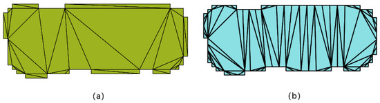
Figure 1.
CDT. (a) Before encryption; (b) after encryption.
According to the classic skeleton line extraction method proposed by DeLucia and Black [11], triangles can be divided into three types (1–3) according to the number of adjacent triangles.
- A type one triangle only has one adjacent triangle, and the two sides are located on the boundary of the building. The triangle marks the end point of the branch of the extracted skeleton line. The midpoint of the adjacent triangle edge and corresponding vertex is connected to obtain the triangular skeleton lines, as indicated by the red line in Figure 2a.
- A type two triangle has two adjacent triangles, one of which is located on the boundary of the polygon, which represents the extension direction of the skeleton line. The midpoint connecting the two adjacent triangle sides is the skeleton line of this type of triangle, as indicated by the red line in Figure 2b.
- A type three triangle has three adjacent triangles, and none of the sides lie on the boundary of the polygon. The skeleton line represents a branch and is formed by connecting the midpoints of the three sides and the center point of the triangle, as indicated by the red line in Figure 2c.

Figure 2.
Triangle classification. (a) Type one; (b) type two; (c) type three.
The skeleton line can be extracted using the classical CDT method for extracting the skeleton line of a vector building. According to the triangle connection method, for every type three triangle in the triangulation, the skeleton line extraction result is expected to have an additional branch, marked in the Figure 3 by the black solid line. However, buildings have few actual branches. Yan [35] abstracted a series of template shapes according to the shape characteristics of the building using common English letters (E, F, L, T, I, and C) and other shapes for building simplification. Furthermore, a building typically has right-angle features, and the skeleton line has few branches. Therefore, the traditional CDT-based skeleton line extraction algorithm is effective for extracting regular graphics. Irregularly processed vector buildings have many noise points, thus, the skeleton line extracted directly using this algorithm has many branches.
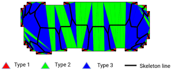
Figure 3.
Skeleton line extraction based on CDT.
2.2. Extracting Skeleton Lines from Raster Data Based on the Rosenfeld Algorithm
In this study, we used the ArcGIS10.4.1 software of Esri company (Redlands, CA, USA) to rasterize vector data. Many skeleton line extraction algorithms have been developed based on raster data. In practical applications, the skeleton line extracted from raster data must have the width of a single pixel and must not change the topology and connectivity of the original building [27]. The fast parallel thinning algorithm based on the ZS method is commonly used at present. However, the thinning result of this algorithm involves redundant pixels, and the thinning is not complete. Jia et al. [36] demonstrated the effectiveness of the Rosenfeld refinement algorithm by comparing the refinement algorithms based on mathematical morphologies (ZS and Rosenfeld). In addition, Zhang et al. [37] compared the performance of the classical thinning algorithms in practical applications and demonstrated the effectiveness of the Rosenfeld algorithm, which is an iterative algorithm. The key concept of raster data thinning is to identify a set of pixels that are equal to the polygon boundary without changing the connectivity relationship of the original polygon.
We used the spatial analysis function of vector data to convert raster skeleton lines into vector data and overlap the original vector buildings for a further analysis. In raster data, row and column numbers were used to indicate the position of the current pixel, whereas, in vector data, coordinates were used to indicate the current point position. The geographic coordinates of the point at the upper left of the raster data, considered as the benchmark, were defined as X, Y, level, vertical, and angle; the latter three represent the horizontal resolution, vertical resolution, and rotation angle, respectively. Then, the formula for converting the raster data point (i, j) to the geographic coordinate point (Xgeo, Ygeo) could be obtained as
Next, the mapping relationship between the raster data points and vector geographic coordinate points was identified. Figure 4 shows the overlay analysis results of skeleton lines extracted using the CDT and Rosenfeld methods.
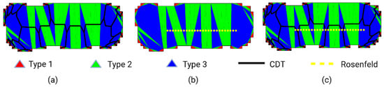
Figure 4.
Skeleton line extraction results. (a) CDT; (b) Rosenfeld; (c) Overlap of CDT and Rosenfeld results.
2.3. Problem Analysis and Research Countermeasures
According to the discussion, the CDT method based on vector data had a strong mathematical theoretical foundation. However, the skeleton line extraction results had many branches and were considerably affected by noise. The extraction results were satisfactory for regular buildings but poor for complex buildings. In comparison, the Rosenfeld skeleton line extraction method based on raster data could better suppress noise. Notably, the methods based on raster data require the data format to be converted, which may decrease the data accuracy, as shown in Figure 4c. Owing to the accuracy loss during data conversion, the skeleton line extracted from raster data was not completely located in the center of the building, which could influence the matching and update operations of the building. In addition, the skeleton line extraction results based on raster data were not optimized for the orthogonal features of buildings. To address these problems, this paper proposes a vector-building extraction method based on vector–raster data integration (VRDI). The CDT method for vector data was used to ensure that the extracted skeleton line was located in the center of the building. The raster data could be easily managed and the noise could be suppressed. The extracted skeleton line maintained only a few building nodes and exhibited obvious orthogonalization characteristics, and the principle of the centrality of the skeleton line was maintained. Figure 5 shows the process flow of the proposed building vector skeleton line extraction method.
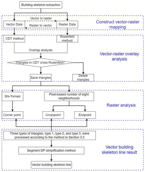
Figure 5.
Process flow of building skeleton line extraction.
3. Proposed Method of Extracting Building Skeleton Line Based on VRDI
3.1. Extraction of the Triangle in Which the Skeleton Line Is Located
The CDT method based on vector data is sensitive to noise interference in complex buildings, resulting in excessive skeleton line branches. In contrast, the skeleton line extraction method based on raster data is not sensitive to noise. To combine the advantages of vector and raster data processing, the data were preprocessed using the overlapping analysis of vector and raster data using the following steps:
- Vectorize the grid skeleton line extracted by the Rosenfeld method and record the line feature as ;
- Traverse all the triangles in the CDT of each building to determine whether the current triangle intersects with in step one. If so, keep the current triangle; otherwise, delete it.
The CDT for the location of the skeleton line was obtained, as shown in Figure 6. The green and blue triangles represent the parts that intersected with the skeleton line, corresponding to the type two and type three triangles of the CDT, respectively. The type one triangle did not affect the final extraction result of the skeleton line.
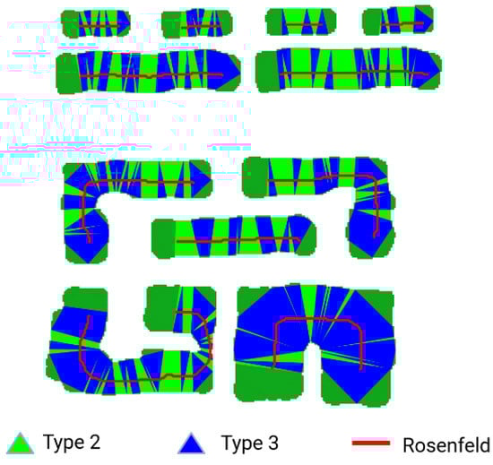
Figure 6.
Extraction of the triangle in which the skeleton line was located.
Buildings typically have right-angled and templated features. To ensure that the right-angled features at the corners were maintained in the skeleton line extraction results, the skeleton lines extracted based on the Rosenfeld method were used for corner detection. This method, while maintaining the details of the building outline, alleviated the problem of traditional CDT methods extracting many branches of the skeleton line.
3.2. Corner Detection Based on Shi–Tomasi Algorithm
The Shi–Tomasi algorithm is a corner detection algorithm that represents an improved version of the Harris algorithm [38]. The basic principle of the algorithm is that a window, , is moved on a grayscale image, , and the grayscale change, , in the image is calculated as
Here, represents the coordinates of the window in the image, and is the pixel value of in the image. The Taylor expansion can be used to rewrite Equation (3) as
where and are the partial differentials of image , and physically represent the gradient map in the and directions, respectively.
where matrix can be expressed as
Let and be the eigenvalues of matrix , and be the corner response function, defined as
Here, is a constant value, usually set as 0.04 to 06. The Shi–Tomasi algorithm takes the minimum values of and based on the Harris algorithm. When is greater than the set threshold, the feature point is retained, and the point is determined to be a strong corner point [39]. The Shi–Tomasi corner detection algorithm is not affected by rotation and satisfies the scale-invariant characteristics. Compared with the Harris corner detection method, it extracts more evenly distributed corners.
In this study, we incorporated the feature of right angles to decrease the false detection rate of corners. The maximum number of corners was set to five. The corner detection results are shown in Figure 7.
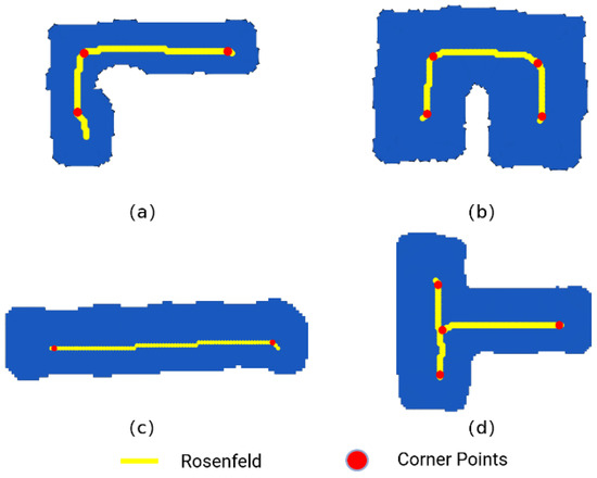
Figure 7.
Corner detection results. (a) L-shaped building; (b) C-shaped building; (c) I-shaped building; (d) T-shaped building.
The traditional CDT-based method to extract vector building skeleton lines generated a branch every time a type three triangle was encountered, and the results were highly susceptible to noise. Specifically, the CDT-based methods produced many branches, owing to the connection method of type three triangles. Type one triangles did not affect the extraction of building skeleton lines. The connection method of type two triangles could ensure that the skeleton line was in the center of the building. Therefore, we modified the CDT-based skeleton line extraction method: First, the endpoints and intersections of the skeleton lines extracted by the Rosenfeld method were detected. Because the skeleton lines were connected by single-pixel width, the eight neighborhood pixels around the pixel value (red arrow in Figure 8) were counted to detect endpoints. If only one foreground point existed, it was the endpoint. The point was a crosspoint if more than two foreground points existed around it.
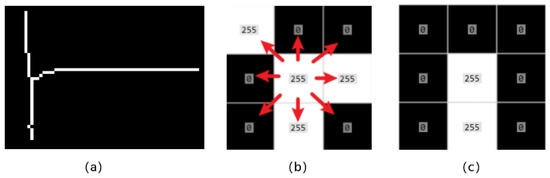
Figure 8.
Detection of endpoints and crosspoints. (a) Rosenfeld skeleton line; (b) Crosspoint; (c) Endpoint.
3.3. Extraction of Building Skeleton Line Based on Vector–Raster Data Integration
Because the main skeleton line of the building did not include type one triangles, the connection method of type two triangles remained unchanged. Therefore, the skeleton line extraction based on the proposed approach involved the following steps:
- Examine whether the three types of triangles contain endpoints, intersections, and corners. If not, four scenarios can be considered.
- If the type three triangles do not contain endpoints, intersections, or corners, as shown in Figure 9b, they are equivalent to type two triangles. Connect the midpoints of the two long sides of this type of triangle, as shown in Figure 9c.
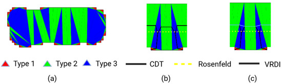 Figure 9. Three type three triangles without endpoints, corners, or intersections. (a) Delaunay triangles classification results; (b) Overlay of Rosenfeld and CDT results; (c) Overlay of Rosenfeld, CDT and VRDI results.
 - If the type three triangles have a crosspoint, as shown in Figure 10a, the skeleton line inevitably branches at a type three triangle. The CDT-based type three triangle connection method changes the original right-angle feature of the building and influences the description of the skeleton line regarding the building shape. However, this method can theoretically prove that the result of the skeleton line extraction is in the center of the vector building and can be used to evaluate the centrality of the skeleton line extraction result, as shown in Figure 10.
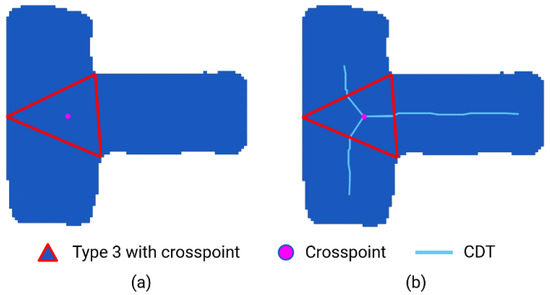 Figure 10. Traditional CDT method for type three triangle connections with a crosspoint. (a) Building with crosspoint; (b) Result of traditional CDT method.
To solve the problems associated with the traditional CDT method of skeleton line extraction, the following conditions must be satisfied when addressing triangles with intersections.
- The skeleton line must pass through the three midpoints of the triangle to maintain the connectivity of the skeleton line extraction results.
- The orientation of the building at the corner must be nearly parallel or perpendicular to the orientation of the building’s minimum bounding rectangle (MBR). Calculate the direction formed by any two midpoints of the three bars and the direction of the MBR; connect two midpoints that are nearly parallel or perpendicular to the direction of the building’s MBR; then, find the projection point of the other midpoint of the triangle on the line. This projection point is the new crosspoint of the skeleton line extracted by the VRDI method, as shown in Figure 11b:
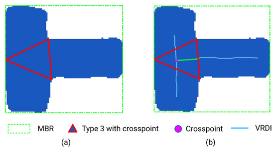 Figure 11. VRDI extraction results. (a) The MBR of building; (b) Result of VRDI method for crosspoint.
- 4.
- Type three triangles with corners: For a vector building with obvious right-angle features, the CDT will have two near-vertical lines. To enhance the generality of the algorithm, the building’s MBR should be used to identify the direction of the building. The black solid line in Figure 12 shows the MBR direction of the building. Let the direction vector of the building be , the center point of the three types of triangles be , and the midpoints of the three sides be , , and respectively. Calculate the absolute value of the cosine of the angle between the vector and vectors , , and . According to the cosine function curve, the absolute value of the cosine of two vectors that are nearly parallel or perpendicular corresponds to the maximum or minimum, and the two edges are connected as a result of the skeleton line extraction.
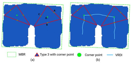 Figure 12. Type three with corner points. (a) C-shaped building with corner point; (b) Result of VRDI method for corner point.
- 5.
- Triangle with endpoints: For a type two triangle, follow the CDT connection method. For a type three triangle, to ensure that the extracted skeleton line is smooth and consistent with the visual characteristics of the human eye, compare the connection method of the previous triangle skeleton line. As shown in Figure 13a, AB is the skeleton line closest to the triangle containing the endpoint, and the skeleton line connection of this triangle must pass through point B to maintain connectivity. There are three possible connection methods: BC, BO, and BD. Calculate the angle between vector and vectors , , and ; then, connect the points corresponding to the direction vector with the smallest angle. The final connection result is shown in Figure 13b.
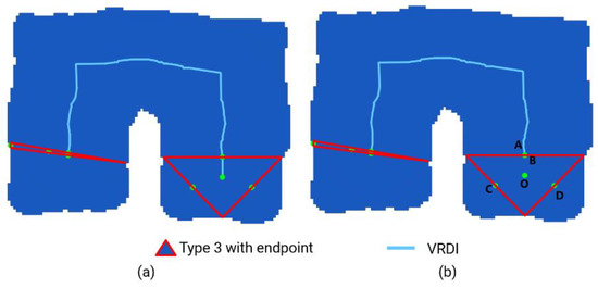 Figure 13. Triangle with endpoints. (a) C-shaped building with endpoint; (b) Result of VRDI method for endpoint.
3.4. Building Skeleton Line Simplification
For regular buildings, the extracted skeleton lines must maintain the original right-angle features of the buildings, and the skeleton line of the vector building must not have many nodes. Notably, the initially extracted building skeleton line had many nodes, and it was difficult to directly describe the characteristics of the building. Therefore, the extracted skeleton line had to be simplified, while satisfying the following requirements:
- The overall shape and connectivity of the original building must not be changed.
- The corner points in skeleton lines cannot be deleted as they are key features of buildings.
- The right-angled feature corners must be maintained.
The segmented Douglas–Peucker (DP) algorithm with corners and crosspoints as the segmentation units was used. The algorithm involves the following steps:
- If the skeleton line does not contain crosspoints, the corner points should be extracted and used as the split point to segment the skeleton line, as shown in Figure 14a,b. If there are crosspoints in the skeleton line, they should be used as the split points to segment the skeleton line, as shown in Figure 14c.
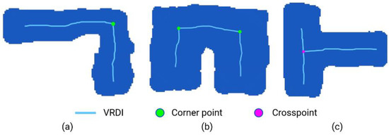 Figure 14. Skeleton line segmentation. (a) L-shaped building with one corner point; (b) C-shaped building with two corner points; (c) T-shaped building with one crosspoint.
 - For each skeleton line, execute the DP algorithm separately.
- Merge the segmentation results to obtain the vector skeleton line of the building.
In this study, the processing results for simplified thresholds of 1 m and 3 m were examined. The results are shown in Figure 15. The red solid lines mark the segmental DP simplification results. Figure 15a–d show the simplified results for the 1 m and 3 m thresholds, respectively. When the threshold was 1 m, the skeleton line was not completely simplified and included redundant nodes. The threshold of 3 m yielded a result that had fewer nodes and could retain the shape characteristics of the original building.
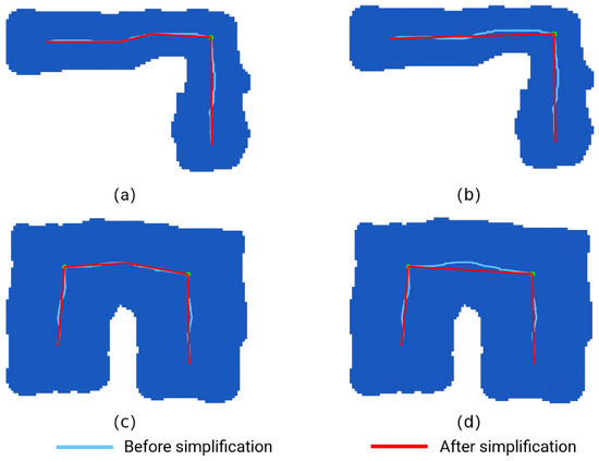
Figure 15.
Skeleton line segment DP simplification results with different threshod; (a) L-shaped building with a threshold of 1 m; (b) L-shaped building with a threshold of 3 m; (c) C-shaped building with a threshold of 1 m; (d) C-shaped building with a threshold of 3 m.
4. Experimental Results and Analysis
4.1. Experimental Results
The effectiveness of the proposed skeleton line extraction method was verified by considering the complex vector buildings initially extracted from high-resolution remote sensing images in the Indianapolis area as the research object. The range of research area from (−86.2001, 39.7444) to (−86.1355, 39.7924) included a total of 10,348 building features. Figure 16a shows the high-resolution remote sensing image, Figure 16b shows the preliminarily extracted vector buildings, and Figure 16c shows the skeleton line extraction results based on the proposed VRDI approach.
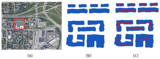
Figure 16.
(a) High-resolution remote sensing images. The highlighted red box area in (a) corresponds to (b,c); (b) Initially extracted vector buildings; (c) Skeleton line extraction results based on the proposed VRDI approach as shown by the red solid line.
For a given research area, in addition to the three common building types I-shaped, L-shaped, and C-shaped in Figure 16, there were also some complex-shaped buildings, such as T-shaped and F-shaped buildings, in Figure 17. In fact, these five typical building shapes were the major shapes in the research area. Therefore, we selected the above five typical building shapes as the research topic.
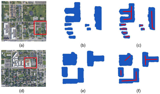
Figure 17.
Skeleton line extraction results for T-shaped and F-shaped buildings. (a) High-resolution remote sensing images. The highlighted red box area in (a) corresponds to (b,c); (b) initially extracted vector buildings; (c) skeleton line extraction results based on the proposed VRDI approach as shown by the red solid line; (d) High-resolution remote sensing images. The highlighted red box area in (d) corresponds to (e,f); (e) initially extracted vector buildings; (f) skeleton line extraction results based on the proposed VRDI approach as shown by the red solid line.
The skeleton line extracted using the traditional CDT method was used as the reference and comparison object (removal of redundant branches). In this experiment, we used three algorithms to perform comparative experiments to evaluate the proposed method. The first two algorithms were the ZS thinning algorithm and the Rosenfeld method, which are the most common methods used in the field of image processing. The third one was the medial axis transform (MAT) method, which could preserve the topological properties of the buildings. However, it was instability to small perturbations of the input buildings that could disturb the topology of the branches [40].
4.2. Skeleton Line Centrality Evaluation Based on the Distance
The distance was used to measure the similarity between curves, and it was determined by minimizing the maximum distance between two curves [41,42]. For two curves, , the Fréchet distance, , could be expressed as follows:
For a given parameter, , we examined whether the distance between two trajectories was less than the parameter . A smaller between the two trajectories corresponded to a smaller distance between two trajectories and a higher degree of similarity. The Fréchet distance between the traditional CDT skeleton line extraction results and that obtained using the Rosenfeld, ZS, MAT, or VRDI methods was used as the index to measure the skeleton line centrality. According to whether the skeleton line extraction results included crosspoints, five types of buildings could be divided into buildings with crosspoints and buildings without crosspoints. The buildings without crosspoints mainly included I-shaped, L-shaped, and C-shaped ones. Buildings with crosspoints were represented by complex geometric shapes, such as T-shaped and F-shaped ones. Figure 18 and Figure 19 show the skeleton extraction results.
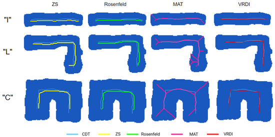
Figure 18.
Building skeleton lines without crosspoints.
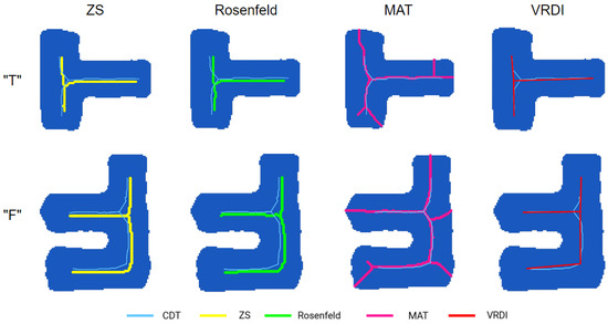
Figure 19.
Building skeleton lines with crosspoints.
The Fréchet distance between the skeleton line extraction results and CDT method extraction results was calculated, as indicated in Table 1. According to the definition of the Fréchet distance, the distance between the two curves is the length of the shortest sufficient for both to traverse their separate paths from start to finish. In other words, a smaller distance corresponds to a skeleton line closer to the center of the building.

As shown in Table 1, the method proposed in this paper significantly outperformed the other three skeleton line extraction algorithms in terms of centrality. The skeleton line extraction methods based on ZS, Rosenfeld, and MAT were based on raster data, and the extraction results could be used to evaluate the directional characteristics of buildings. However, for raster data, the basic processing unit was the pixel, and the processing result was closely related to the resolution of the image. In contrast, the basic unit of vector data processing was point data. In the spatial analysis of GIS, point data only represent the location characteristics of attributes. In the skeleton line extraction based on raster data, maintaining the connectivity of the results was the precondition for skeleton line extraction. Therefore, the skeleton line extraction method based on raster data usually had difficulty satisfying the centrality constraint.
4.3. Evaluation of Skeleton Line Direction Based on the MBR
The buildings had obvious directional characteristics, and the skeleton line is a simplified expression of the overall shape of the building. Therefore, the orientation of the skeleton line extraction result had to be consistent with the orientation of the original building. In this study, the long side of a building’s MBR was defined as the direction of the building. The MBR is typically used to represent the direction feature of a simple polygon [43,44]. In practical applications, the MBR is only used to describe the direction of a simple polygon, such as an I-shaped or C-shaped one. For complex buildings, using the MBR to measure the direction of the building would cause a large loss of accuracy. Shen [45] first divided buildings into orthogonal and nonorthogonal features in the direction of measuring the buildings, and the main orientation of buildings had to be the same as the direction of one line segment connected by two adjacent corners arranged clockwise or counter-clockwise along the edge of the original buildings. For buildings with nonorthogonal features, the main orientation could be confirmed through the calculation of the image moment [46]. In this study, we used the MBR as the approximate orientation of the buildings for analysis. The angle formed by the long side of the MBR and Y-axis direction was the angle of the building. The angle of the original building and angle differences among the three methods were calculated to extract the skeleton line and analyze the direction-change characteristics of the three types of skeleton line extraction methods.
Vector skeleton lines only had a length, while buildings had both length and width dimensions. Therefore, the MBR of a complex building may have shown a large difference in terms of the orientation of the MBR of the skeleton line. As shown in Figure 20, the MBR of the T-shaped building was considerably different to that of the skeleton line. However, the MBRs of the F-shaped building and skeleton line were in the same direction. The reason for this phenomenon was that the MBR was obtained by rotating the circumscribed rectangle. The MBR needed to calculate the enclosing rectangle of the polygon first, then rotate the enclosing rectangle according to a certain step size until the area of the enclosing rectangle was the smallest. The obtained enclosing rectangle was called the MBR.
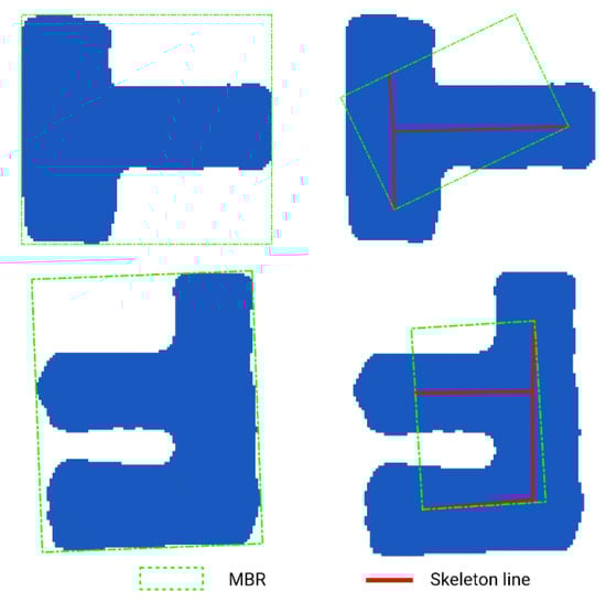
Figure 20.
MBR for buildings and skeleton lines.
In this study, we considered five typical shapes of buildings to calculate the angle between buildings and skeleton lines. The calculation results are presented in Table 2.
We analyzed and evaluated the three skeleton line extraction methods in terms of the centrality and direction change of skeleton lines. The proposed method could maintain the centrality of the skeleton line, and the direction of the skeleton line extraction results and the original building was similar. The proposed method combined the advantages of vector data and raster data in a spatial analysis. The extracted skeleton line could retain the right-angle characteristics of buildings and consider the centrality characteristics of skeleton lines. The proposed method outperformed the ZS, MAT, Rosenfeld, and traditional CDT methods in processing building corners and crosspoints.
5. Conclusions
Vector building skeleton lines are widely used in building matching and updating in GIS applications. The proposed method combined the advantages of vector data and raster data in extracting skeleton lines and could solve the problems that the traditional CDT-based skeleton line extraction results had many branches and that the orthogonal features of the raster data skeleton line extraction results were not obvious. The experimental results showed that the proposed skeleton line extraction method could better maintain the orthogonal characteristics of the buildings. The skeleton line extraction results exhibited few branches and insensitivity to noise, even in the case of complicated buildings. Notably, the vector buildings extracted from high-resolution remote sensing images could contain holes; thus, a lot of the holes should have been filled first. Moreover, since the parameter setting of the number of corner points is very important, how to adaptively set more accurate parameters should be a topic for future research.
Author Contributions
Conceptualization, Guoqing Chen and Haizhong Qian; methodology, Guoqing Chen and Haizhong Qian; software, Guoqing Chen; validation, Guoqing Chen and Haizhong Qian; formal analysis, Guoqing Chen; investigation, Haizhong Qian; resources, Haizhong Qian; data curation, Guoqing Chen; writing—original draft preparation, Guoqing Chen; writing—review and editing, Guoqing Chen and Haizhong Qian; visualization, Guoqing Chen; supervision, Haizhong Qian; project administration, Guoqing Chen and Haizhong Qian; funding acquisition, Haizhong Qian. All authors have read and agreed to the published version of the manuscript.
Funding
This research was funded by The Natural Science Foundation for Distinguished Young Scholars of Henan Province, grant number 212300410014.
Data Availability Statement
Not applicable.
Conflicts of Interest
The authors declare no conflict of interest.
References
- Lu, T.; Ming, D.; Lin, X.; Hong, Z.; Bai, X.; Fang, J. Detecting building edges from high spatial resolution remote sensing imagery using richer convolution features network. Remote Sens. 2018, 19, 1496. [Google Scholar] [CrossRef]
- Ai, T.; Liu, Y. Aggregation and amalgamation in land-use data generalization. Geomat. Inf. Sci. Wuhan Univ. 2002, 27, 486–492. [Google Scholar]
- Cai, Y.; Ming, C.; Qin, Y. Skeleton extraction based on the topology and Snakes model. Results Phys. 2017, 7, 373–378. [Google Scholar] [CrossRef]
- Ai, T.; Yang, F.; Li, J. Land-use data generalization for the database construction of the second land resource survey. Geomat. Inf. Sci. Wuhan Univ. 2010, 35, 887–891. [Google Scholar]
- Qian, H.Z.; Wu, F.; Ge, L.; Wang, J.Y. Quality assessment of city-building geometry-generalization with reducing-dimension technique. J. Image Graph. 2007, 5, 927–934. [Google Scholar]
- Ai, T.; Zhang, X.; Zhou, Q.; Yang, M. A vector field model to handle the displacement of multiple conflicts in building generali-zation. Int. J. Geogr. Inf. Sci. 2015, 29, 1310–1331. [Google Scholar] [CrossRef]
- Bertasius, G.; Shi, J.; Torresani, L. High-for-Low and Low-for-High: Efficient Boundary Detection from Deep Object Features and Its Applications to High-Level Vision. In Proceedings of the 2015 IEEE International Conference on Computer Vision (ICCV), Santiago, Chile, 7–13 December 2015. [Google Scholar] [CrossRef]
- Shen, W.; Wang, X.; Wang, Y.; Bai, X.; Zhang, Z. Deepcontour: A deep convolutional feature learned by positive-sharing loss for contour detection. In Proceedings of the IEEE Conference on Computer Vision and Pattern Recognition, Boston, MA, USA, 7–12 June 2015; pp. 3982–3991. [Google Scholar]
- Wang, Y.; Zhao, X.; Li, Y.; Huang, K. Deep Crisp Boundaries: From Boundaries to Higher-Level Tasks. IEEE Trans. Image Process. 2018, 28, 1285–1298. [Google Scholar] [CrossRef]
- Widyaningrum, E.; Gorte, B.; Lindenbergh, R.C. Automatic Building Outline Extraction from ALS Point Clouds by Ordered Points Aided Hough Transform. Remote Sens. 2019, 11, 1727. [Google Scholar] [CrossRef]
- DeLucia, A.A.; Black, R.T. A comprehensive approach to automatic feature generalization. In Proceedings of the 13th Con-ference of the International Cartographic Association, Morelia, Mexico, 12–21 October 1987; pp. 173–191. [Google Scholar]
- Morrison, P.; Zou, J.J. Triangle refinement in a constrained Delaunay triangulation skeleton. Pattern Recognit. 2007, 40, 2754–2765. [Google Scholar] [CrossRef]
- Jones, C.B.; Bundy, G.L.; Ware, M.J. Map generalization with a triangulated data structure. Cartogr. Geogr. Inf. Syst. 1995, 22, 317–331. [Google Scholar]
- McAllister, M.; Snoeyink, J. Medial Axis Generalization of River Networks. Cartogr. Geogr. Inf. Sci. 2000, 27, 129–138. [Google Scholar] [CrossRef]
- Regnauld, N.; Mackaness, W.A. Creating a hydrographic network from its cartographic representation: A case study using Ordnance Survey MasterMap data. Int. J. Geogr. Inf. Sci. 2006, 20, 611–631. [Google Scholar] [CrossRef]
- Wang, Z.H.; Yan, H.W. Design and implementation of an algorithm for extracting the main skeleton lines of polygons. Geogr. Geoinf. Sci. 2011, 27, 42–44. [Google Scholar]
- Shen, L.H.; Wu, B.G.; Yang, N. Areal feature main skeleton extraction algorithm. Geomat. Inf. Sci. Wuhan Univ. 2014, 39, 767–771. [Google Scholar] [CrossRef]
- Li, C.; Yin, Y.; Wu, P.; Wu, W. Skeleton Line Extraction Method in Areas with Dense Junctions Considering Stroke Features. ISPRS Int. J. Geo-Inf. 2019, 8, 303. [Google Scholar] [CrossRef]
- Wang, Z.H.; Yan, H.W. An algorithm for extracting main skeleton lines of polygons based on main extension directions. In Proceedings of the 2011 International Conference on Electronics, Communications and Control (ICECC), Ningbo, China, 9–11 September 2011; pp. 125–127. [Google Scholar]
- Zhang, T.Y.; Suen, C.Y. A fast parallel algorithm for thinning digital patterns. Commun. ACM 1984, 27, 236–239. [Google Scholar] [CrossRef]
- Pavlidis, T. Algorithms for Graphics and Image Processing, 1st ed.; Springer: Berlin/Heidelberg, Germany; New York, NY, USA, 1982; p. 438. [Google Scholar]
- Rosefeld, A.; Kak, A. Digital Picture Processing; Academic Press: New York, NY, USA, 1982. [Google Scholar]
- Holt, C.M.; Stewart, A.; Clint, M.; Perrott, R.H. An improved parallel thinning algorithm. Commun. ACM 1987, 30, 156–160. [Google Scholar] [CrossRef]
- Chen, W.; Sui, L.; Xu, Z.; Lang, Y. Improved Zhang-Suen thinning algorithm in binary line drawing applications. In Proceedings of the 2012 International Conference on Systems and Informatics, Yantai, China, 19–20 May 2012; pp. 1947–1950. [Google Scholar] [CrossRef]
- Ben Boudaoud, L.; Solaiman, B.; Tari, A. A modified ZS thinning algorithm by a hybrid approach. Vis. Comput. 2017, 34, 689–706. [Google Scholar] [CrossRef]
- Jagna, A. An Efficient Image Independent Thinning Algorithm. IJARCCE 2014, 3, 8309–8311. [Google Scholar] [CrossRef]
- Tarabek, P. A robust parallel thinning algorithm for pattern recognition. In Proceedings of the 2012 7th IEEE International Symposium on Applied Computational Intelligence and Informatics (SACI), Timisoara, Romania, 24–26 May 2012; pp. 75–79. [Google Scholar] [CrossRef]
- Blum, H. A transformation for extracting new descriptors of shape. Model. Preception Speech Vis. 1967, 19, 362–380. [Google Scholar]
- Widyaningrum, E.; Peters, R.Y.; Lindenbergh, R.C. Building outline extraction from ALS point clouds using medial axis transform descriptors. Pattern Recognit. 2020, 106, 107447. [Google Scholar] [CrossRef]
- Ben Boudaoud, L.; Sider, A.; Tari, A. A new thinning algorithm for binary images. In Proceedings of the 2015 3rd International Conference on Control, Engineering & Information Technology (CEIT), Tlemcen, Algeria, 25–27 May 2015. [Google Scholar] [CrossRef]
- Klein, R. Voronoi Diagrams and Delaunay Triangulations; World Scientific: Singapore, 2013. [Google Scholar]
- Shen, Y.; Ai, T. A Hierarchical Approach for Measuring the Consistency of Water Areas between Multiple Representations of Tile Maps with Different Scales. ISPRS Int. J. Geo-Inf. 2017, 6, 240. [Google Scholar] [CrossRef]
- Kocharyan, D. An Efficient Fingerprint Image Thinning Algorithm. Am. J. Softw. Eng. Appl. 2013, 2, 1–6. [Google Scholar] [CrossRef][Green Version]
- Shen, Y.; Ai, T.; Yang, M. Extracting Centerlines from Dual-Line Roads Using Superpixel Segmentation. IEEE Access 2019, 7, 15967–15979. [Google Scholar] [CrossRef]
- Yan, X.F.; Ai, T.H.; Yang, M. A simplification of residential feature by the shape cognition and template matching method. Acta Geo. Cartogr. Sin. 2016, 45, 874–882. [Google Scholar]
- Jia, T.M.; Xun, Y.; Bao, G.J.; Done, M.; Yang, Q.H. Skeleton extraction algorithm on grapevine based on machine vision. J. Mech. Electr. Eng. 2013, 30, 501–504. [Google Scholar]
- Zhang, R.; Wang, S.Y.; Liu, S.L.; Shi, S.Q.; Zhou, J. Automatic extraction for geographic national conditions water elements. Geomat. Spat. Inf. Technol. 2015, 38, 59–61. [Google Scholar]
- Shi, J.; Tomasi, C. Good Features to Track. In Proceedings of the IEEE Conference on Computer Vision and Pattern Recognition, Seattle, WA, USA, 21–23 June 1994; pp. 593–600. [Google Scholar]
- Chang, J.; Wang, S.; Yang, Y.; Gao, X. Hierarchical optimization method of building contour in high-resolution remote sensing image. Chin. J. Lasers 2020, 47, 249–262. [Google Scholar]
- Bai, X.; Latecki, L.J.; Liu, W.Y. Skeleton Pruning by Contour Partitioning with Discrete Curve Evolution. IEEE Trans. Pattern Anal. Mach. Intell. 2007, 29, 449–462. [Google Scholar] [CrossRef]
- Fréchet, M.M. Sur quelques points du calcul fonctionnel. Rend. Circ. Matem. Palermo 1906, 22, 1–72. [Google Scholar] [CrossRef]
- Luo, G.W.; Zhang, X.C.; Qi, L.X.; Guo, T.S. The fast Positioning and Optimal Combination Matching Method of Change Vector Object. Acta Geod. Cartogr. Sin. 2014, 43, 1285–1292. [Google Scholar]
- Duchêne, C.; Bard, S.; Barillot, X.; Ruas, A.; Trevisan, J.; Holzapfel, F. Quantitative and qualitative description of building orientation. In Proceedings of the 5th Workshop on Progress in Automated Map Generalization, ICA, Commission on Map Generalization, Paris, France, 28–30 April 2003. [Google Scholar]
- Wang, X.; Burghardt, D. A typification method for linear building groups based on stroke simplification. Geocarto Int. 2019, 36, 1732–1751. [Google Scholar] [CrossRef]
- Shen, Y.; Ai, T.; Li, C. A simplification of urban buildings to preserve geometric properties using superpixel segmentation. Int. J. Appl. Earth Obs. Geoinf. 2019, 79, 162–174. [Google Scholar] [CrossRef]
- Hu, M.K. Visual pattern recognition by moment invariants. IRE Trans. Inf. Theory 1962, 8, 179–187. [Google Scholar]
Publisher’s Note: MDPI stays neutral with regard to jurisdictional claims in published maps and institutional affiliations. |
© 2022 by the authors. Licensee MDPI, Basel, Switzerland. This article is an open access article distributed under the terms and conditions of the Creative Commons Attribution (CC BY) license (https://creativecommons.org/licenses/by/4.0/).