A Forest of Forests: A Spatially Weighted and Computationally Efficient Formulation of Geographical Random Forests

Abstract

The aim of this paper is to present developments of an advanced geospatial analytics algorithm that improves the prediction power of a random forest regression model while addressing the issue of spatial dependence commonly found in geographical data. We applied the methodology to a simple model of mean household income in the European Union regions to allow easy understanding and reproducibility of the analysis. The results are encouraging and suggest an improvement in the prediction power compared to previous techniques. The algorithm has been implemented in R and is available in the updated version of the SpatialML package in the CRAN repository.

1. Introduction

Spatial adaptations of machine learning (ML) algorithms have become popular in the past few years. From a prediction-oriented perspective, spatial data contain properties that can be difficult to tackle with traditional statistical techniques due to issues with non-linearity and variable selection. On the contrary, ML algorithms are more flexible due to their non-parametric nature and better performance with highly dimensional data.

Recent efforts to construct reliable and interpretable spatial formulations of commonly used ML algorithms for tabular data such as random forest (RF), presented as publicly available scientific software, started with Hengl et al. [1] and Georganos et al. [2]. At the same time, they represent the main conceptual differences within the spatial ML domain—using spatial variables to inform spatial interactions versus using spatially local models.

Starting with the former, Hengl et al. [1] proposed the inclusion of geographical variables in the forms of distances within a random forest (RF) framework to address spatiotemporal heterogeneity with remarkable success over aspatial models. In this framework, the ML algorithm is considered a satisfactory solution, but the problem lies in the lack of appropriate data to learn the spatial interactions in place. Following on that track, other adaptations have emphasized the use of spatial covariates as input to ML algorithms, to increase predictive prowess [3]. Sekulić et al. [4] proposed the inclusion of distances between observations as an additional variable to enhance the quality of a spatial interpolation task, with some success when compared to popular interpolators such as kriging, while similar work was proposed by Ahn [5]. Xia et al. [6] included spatiotemporal lags as input in the RF model to model drug-related crime patterns in the US. Recently, Saha et al. [7] proposed RF-GLS, an adaptation of RF that captures spatial interaction by estimating non-linear effects in spatial data through Gaussian processes, which substantially outperformed the default model. Similarly, Talebi et al. [8] developed spatial random forests (SRF), which includes non-parametric higher-order spatial statistics in the formulation of RF. Notably, Ancell and Bean [9] proposed the formulation of spatially aware autoregressive trees where the spatial qualities of the data are captured while developing the tree by spatially guided partitions. In general, relying on spatial covariates based on training data locations to improve the results shows remarkable potential but faces limitations such as overfitting if the sampling of the training data is very skewed and imbalanced [10].

The alternative conceptual approach, proposed by Georganos et al. [2] and named geographical random forest (GRF), suggests that the spatial interaction can be captured by an ensemble of local models, rather than focusing on including extensive spatial predictors in a single, global model. This process reflects the concept of geographically varying models such as geographically weighted regression (GWR) [11], which have been very popular in the field of geocomputation since the early 2000s. Although GRF was initially deployed for population mapping through Earth Observation (EO) data, it has since been used for leaf trait mapping using Sentinel 2 satellite data [12], modelling ice extent [13], tree canopy height [14], locations of unconventional wells [15], agricultural draught assessment [16] and landslide susceptibility [17]. It has also found merit in the field of spatial epidemiology where it was used to predict the spatial distribution of type-two diabetes prevalence across the US [18]. Similar methodological approaches have additionally been proposed using spatial quantile random forests [19,20], inverse distance weighted forests or boosting trees [21,22], interpretable spatiotemporal random forests [23] or mixed GWR-RF approaches [24].

In this communication, we present the latest developments of the GRF algorithm through the R package “SpatialML”. We tackle three issues: (i) spatial weighting, (ii) bandwidth optimization and (iii) computational efficiency. In the initial formulation of the “SpatialML” package, GRF was not parallelized, while no weighting was foreseen for the sub-models, meaning that all observations within each local sub-model were weighted equally. Additionally, no solutions regarding an approach to optimize the bandwidth and, hence, the spatial scale of the analysis, have been presented yet. Consequently, in this work we address these issues using a public dataset and presenting a comparative analysis with other popular spatial analysis methods.

2. Materials and Methods

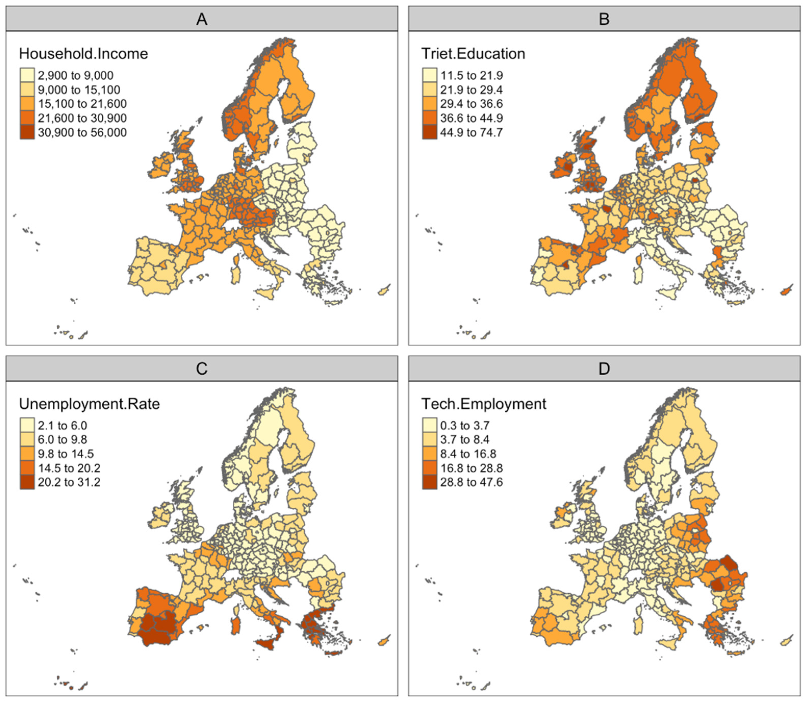
2.1. Dataset

The data analyzed for the purpose of this paper refer to the regions of the European Union of 28 Member States (before Brexit). The geographical boundaries of the EU regions are legally defined as the Nomenclature of Territorial Units for Statistics (NUTS) 2016, Level 2 (NUTS2). There are several versions of this geographical dataset (based on the publication year, scale, coordinate system, etc.). The specific shapefile used here refers to 2016 and has a geographical scale of 1:3,000,000 and the projection EPSG:3035—ETRS89/LAEA Europe. The boundary data are available from the Geographic Information System of the Commission (GISCO). The geographical coordinates used in the analysis of this paper refer to the geometric centroids of the spatial polygons of this shapefile (geometric centroid of each EU region) and were computed using QGIS functions.

This shapefile is linked to a table of four socioeconomic variables and together they constitute the dataset for this analysis. During the data cleaning process, a small number of regions were removed due to missing socioeconomic data. The final dataset comprises 264 observations. The dependent variable refers to the income of households by NUTS 2 regions (Eurostat table code NAMA_10R_2HHINC) (Available online: https://appsso.eurostat.ec.europa.eu/nui/show.do?dataset=nama_10r_2hhinc&lang=en, accessed on 15 June 2022) and its calculation is based in the regional accounts of 2016. After preliminary analysis, three independent variables were selected for the models: total unemployment rate; the proportion of tertiary education of the population; and the rate of employment in technology and knowledge-intensive sectors.

The total unemployment rate refers to people aged 20 to 64 years old and comes from the table “Unemployment rates by sex, age and NUTS 2 regions (%) (code LFST_R_LFU3RT)” (Available online: https://ec.europa.eu/eurostat/databrowser/view/LFST_R_LFU3RT/default/table?lang=en, accessed on 15 June 2022). The source for these data is the EU Labour Force Survey (EU-LFS) for the year 2016. The data on tertiary education came from the table “Population by educational attainment level, sex and NUTS 2 regions (%) (code: EDAT_LFSE_04)” (Available online: https://appsso.eurostat.ec.europa.eu/nui/show.do?dataset=edat_lfse_04&lang=en, accessed on 15 June 2022) and refer to people aged 25 to 64 years old. The values are annual averages of quarterly EU Labour Force Survey data (EU-LFS) for the year 2016. The data of the third explanatory variable came from the table “Employment in technology and knowledge-intensive sectors by NUTS 2 regions and sex (code: htec_emp_reg2)” (Available online: https://appsso.eurostat.ec.europa.eu/nui/show.do?dataset=htec_emp_reg2&lang=en, accessed on 15 June 2022). The latter is part of the statistics on high-tech industry and knowledge-intensive services, which have multiple raw data sources. The source of all these data is Eurostat, European Commission and they are freely available through the Eurostat website. The spatial distribution of the variables is illustrated in Figure 1.

2.2. Models

The model defined in our analysis is a simple income model in which the regional mean household disposable income is regressed over the total unemployment rate, the proportion of economically active people with tertiary education and the proportion of workers in technology and knowledge-intensive sectors. The purpose of this model is to allow an easy-to-understand illustration of the application of the proposed methodology. Based on social science theory and previous findings, we expect unemployment rate to have a negative impact on household income and high educational attainment level to have a positive impact on household income [25] at the regional level.

2.2.1. Geographical Random Forest

The first implementation and development of GRF was presented in detail in Georganos et al. [2]. GRF is an ensemble of locally calibrated random forest (RF) models. The equation for the calibration is presented below [2].

$${\mathrm{Y}}_{\mathrm{i}}=\mathrm{a}\left({\mathrm{u}}_{\mathrm{i}},{\mathrm{v}}_{\mathrm{i}}\right){\mathrm{x}}_{\mathrm{i}}+\mathrm{e},\hspace{1em}\mathrm{i}=1:\mathrm{n}$$

(1)

where $\mathrm{a}\left({\mathrm{u}}_{\mathrm{i}},{\mathrm{v}}_{\mathrm{i}}\right){\mathrm{x}}_{\mathrm{i}}$ refers to the training of an RF model that is applied on location i with $\left({\mathrm{u}}_{\mathrm{i}},{\mathrm{v}}_{\mathrm{i}}\right)$ being the geographical coordinates. The locally developed RF models only use a certain amount of neighboring data points to train the model. The way nearest data points are included in the local models is through the nearest neighbor method, and the maximum number of neighbors that are used to calibrate the local models is called the bandwidth. For inference on a given spatial location, the nearest local RF model is used, with the choice of having a global RF model using all data points to contribute to the prediction.

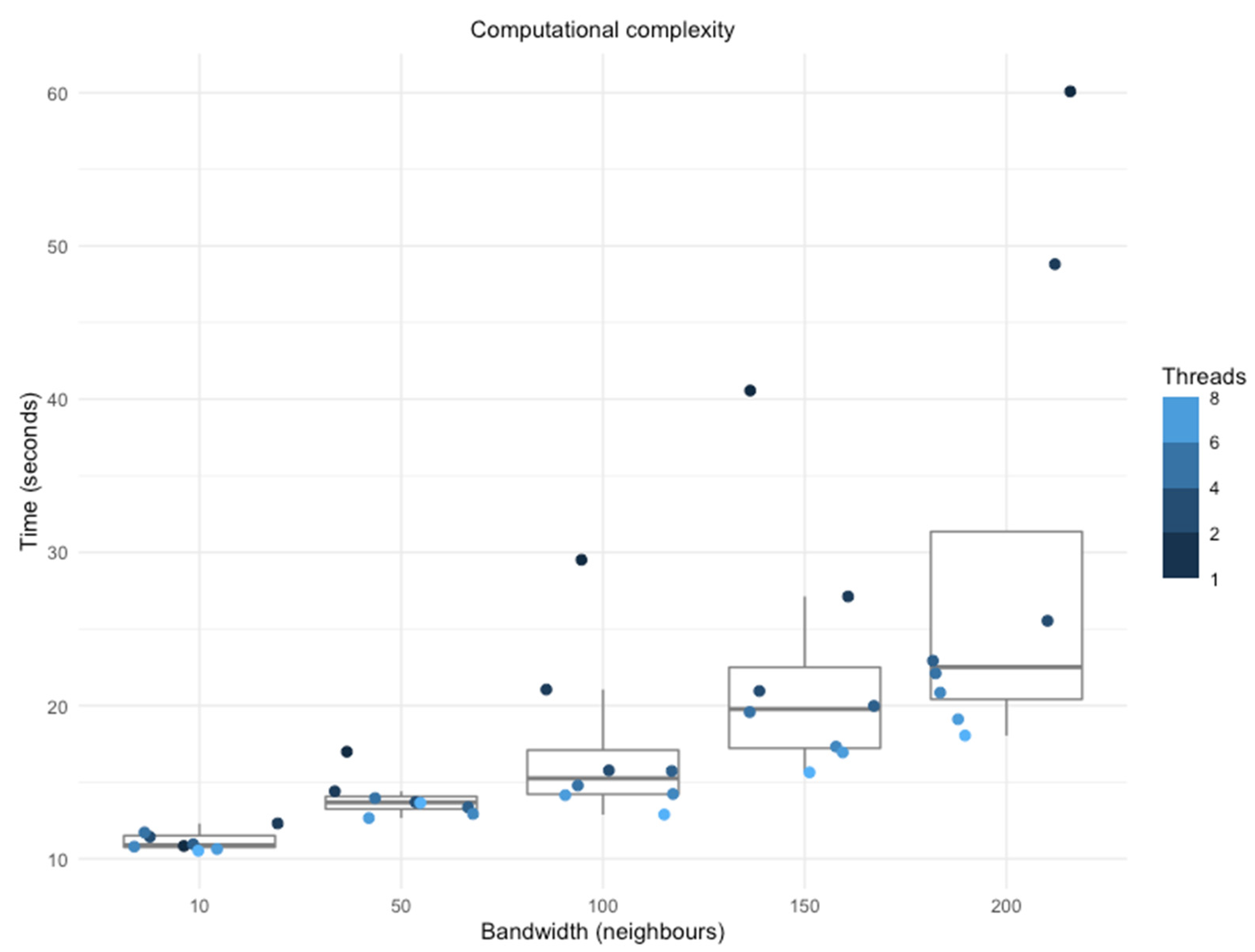
GRF Computational Efficiency

A point of interest is the computational efficiency of the algorithm. The first implementation of GRF on the “SpatialML” package was not parallelizable, which caused long computing times when using large bandwidths or amounts of training data. In the new implementation, we make use of the “ranger” R package to develop the local and global RF models, which are parallelizable. Hence, we investigate the computational gains in terms of computing time in various bandwidths to demonstrate its efficiency.

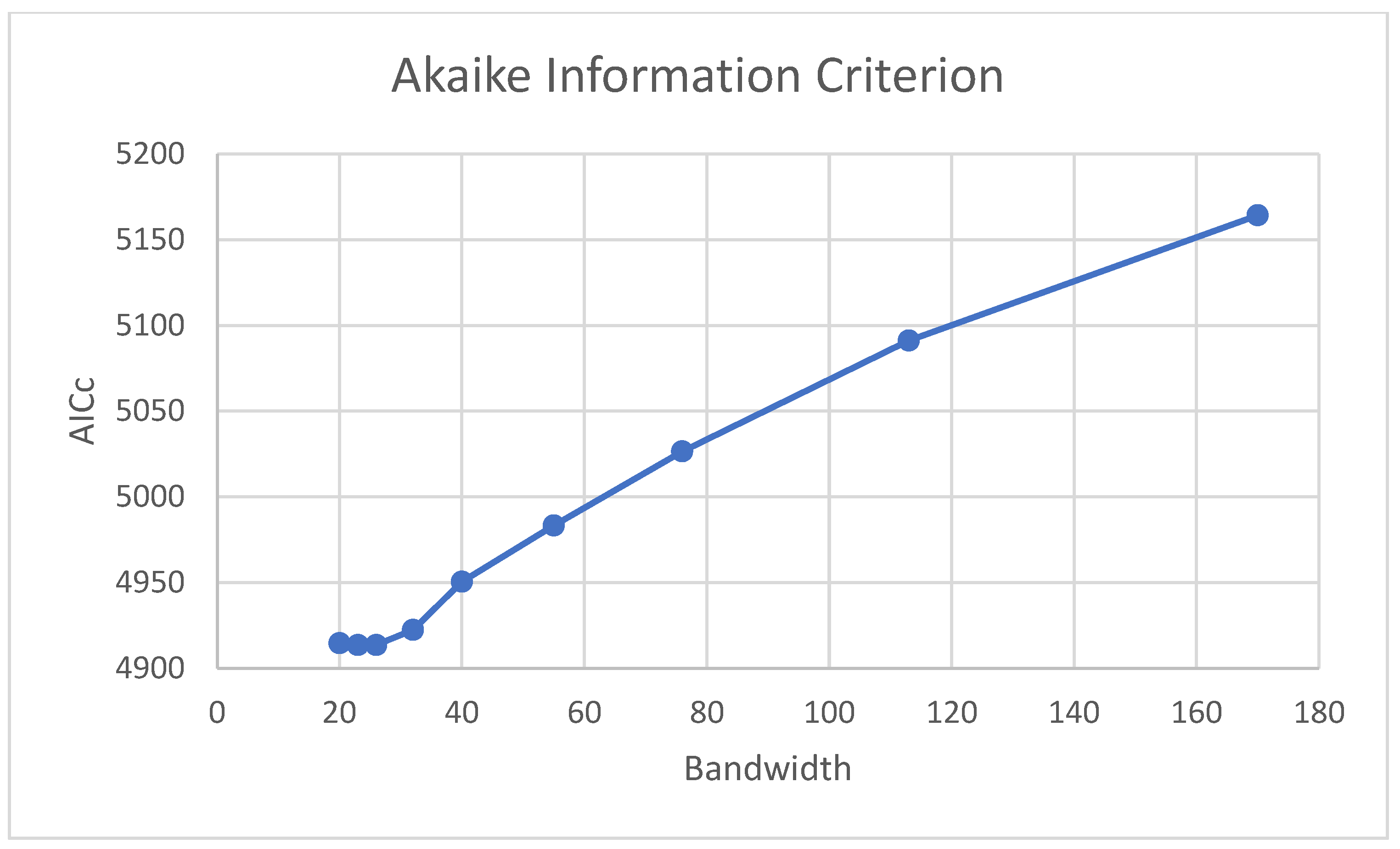
GRF Bandwidth Optimization

One of the challenges in GRF development is to adequately identify optimal bandwidths, which reflects the appropriate spatial scale to model the data. In GRF, bandwidth optimization can be a tedious process based on trial-and-error approaches. To mitigate this issue, we propose a procedure to select an optimal bandwidth using the out-of-bag (OOB) accuracy of GRF. More specifically, we extract the OOB accuracy across various bandwidths and select the one with the best performance. In this example, we selected a bandwidth range starting from 20 to 50 as a proof of concept. Smaller bandwidth values can cause unstable results as the local sub-models are trained with insufficient sample sizes to infer robust parameters.

Spatial Weighting

One of the new developments presented here is the option to spatially weight the local observations. A spatial weights matrix is constructed, used as input in each of the local models. The spatial weights matrix is used as input to the “case.weights” parameter of the “ranger” implementation, allowing data points with larger weights to be selected with higher probability in the bootstrapping procedure of the decision trees [26]. We hereby denote this implementation as GRF-W. The initial implementation of GRF suffered from the shortcoming that all data points within the bandwidth were weighted equally. Consequently, one of the aims is to compare the potential improvement of spatial weighting in the prediction capability.

2.2.2. Benchmark Models and Validation Metrics

We used a set of well-known and commonly employed models to compare the predictive potential of the GRF algorithm with, namely geographically weighted regression (GWR) [27], random forest (RF) [28] and ordinary least squares (OLS) regressors. GWR has several established frameworks to optimize the bandwidth selection. In this work, we used the optimization function from the “GWmodel” in R which identifies the appropriate bandwidth value using the Akaike Information Criterion (AIC) as a performance indicator. The parameters for RF were calibrated through the “caret” R package [29]. Finally, for validation we used the mean absolute error (MAE), root mean squared error (RMSE) and coefficient of determination (R²), as they are commonly used to evaluate regression analyses [30].

3. Results

3.1. GRF and GWR Bandwidth Optimization

Figure 2 illustrates the results of the bandwidth optimization for the GRF models. Using the OOB R² as an anchor, the peak performance was achieved using a bandwidth of 20 neighbors with a constant decline as the number of neighbors increased. We used the same bandwidth parametrization for both GRF and GRF-W. The optimal bandwidth for GWR, based on the AIC, was detected with 23 neighbors (Figure 3).

3.2. Predictive Performance

The results of the validation analysis using various performance indicators are demonstrated in

Table 1. Predictive performance of the models on validation data.

	OLS	RF	GRF	GRF-W	GWR
RMSE	5024.7	4104.6	3071.2	2801.5	3259.00
MAE	3949.6	2578.7	1763.2	1580.4	1933.6
R2	0.45	0.61	0.79	0.82	0.77

. Evidently, aspatial models did not perform well, as both OLS and RF exhibited moderate R² (0.45 and 0.61, respectively), RMSE (5024.7 and 4104.6) and MAE (3949.6 and 2578.7) values. On the contrary, spatial models performed remarkably better. GWR and the traditional GRF implementation demonstrated highly accurate performances, with the former exhibiting a higher R² of 0.77 while the latter exhibited an R² value of 0.79. However, the newly proposed implementation (GRF-W) performed the best, with an R² of 0.82, highlighting the merits of spatial weighting during the bootstrapping process in highly heterogeneous datasets.

3.3. Computational Improvements

Enabling parallelization through the “ranger” package in R drastically reduced computing time in the training of the GRF models. The benefits of parallelization appear to increase linearly with the bandwidth size. This was most evident in larger bandwidths, where a GRF model running on eight computing threads and 200 neighbors required 18 s to compute, whereas more than a minute was required when running on a single thread (Figure 4). Nonetheless, the improvements are minimal in very small bandwidth sizes, likely due to overhead issues.

4. Discussion and Conclusions

In this communication, we present the latest developments in the widely used GRF algorithm [2]. An important bottleneck of the algorithm was its high computational complexity in comparison to simpler approaches such as a global RF or GWR models. To mitigate this issue, we enabled multi-thread parallelization by replacing the “random forest” RF implementation in R with the “ranger” package. Our analysis demonstrated that parallelization is very beneficial, with moderate-to-large bandwidths, but provides little to no benefit for very small ones. This is an artifact of the overhead limitations, as by using small bandwidth values, the computation is very fast and efficient even with one computing thread. A challenge that remains is the memory usage when the sample size increases. As a local RF model is computed and stored for each training data point, the memory requirements can become untenable for large sample sizes. One way this can be solved is by avoiding the storage of the local models as objects during the training process, but only saving necessary information for performance evaluations and inferences. Solving this issue can enable GRF to scale adequately when using larger data volumes.

In our analysis, we demonstrated the importance of spatially weighting the observations within the kernels of the local models. Even though the initial GRF formulation operates with spatial subsets of the training data, all observations within the kernels were weighted equally. In typical GWR models, the observations closer to the training data points receive higher weights than those further away, which essentially turns the local OLS regressors into a spatially weighted OLS. In GRF, the model is the highly non-linear average of several independent decision trees with bootstrapped samples and thus an alternative approach was proposed—to select observations closer to the training data points more frequently in the bootstrapping process rather than those further away. The weighted variant significantly improved the results with roughly a 0.05 increase in the coefficient of determination. Alternative weighting approaches may further improve the results and should be investigated.

Identifying a suitable spatial scale (bandwidth parameter) in GRF can be a challenging task. The proposed automatic optimization using the OOB accuracy metrics exhibited good results, as the models identified as optimal outperformed benchmark approaches. Nonetheless, while the OOB accuracy acts as a pseudo-independent metric, it can be biased [31]. Alternative methods such as cross-validation could be better performing while at the same time being applicable to other types of algorithms that do not have embedded measures of performance such as RF.

ML algorithms are becoming increasingly applied in geospatial analytics instead of more traditional statistical approaches. One challenge with ML approaches is the increased difficulty to extract inferences. For instance, a typical OLS or GWR model can be interpreted relatively easy using linear coefficients but the same cannot be said for RF. Future efforts to improve spatial ML should focus on improving the interpretability of the predictive variables in terms of coefficient and importance, as well as feature selection.

References

1. Hengl, T.; Nussbaum, M.; Wright, M.N.; Heuvelink, G.B.M.; Gräler, B. Random Forest as a Generic Framework for Predictive Modeling of Spatial and Spatio-Temporal Variables. PeerJ 2018, 6, e5518. [Google Scholar] [CrossRef] [PubMed]
2. Georganos, S.; Grippa, T.; Gadiaga, A.N.; Linard, C.; Lennert, M.; Vanhuysse, S.; Mboga, N.O.; Wolff, E.; Kalogirou, S. Geographical Random Forests: A Spatial Extension of the Random Forest Algorithm to Address Spatial Heterogeneity in Remote Sensing and Population Modelling. Geocarto Int. 2019, 36, 121–136. [Google Scholar] [CrossRef]
3. Mariano, C.; Mónica, B. A Random Forest-Based Algorithm for Data-Intensive Spatial Interpolation in Crop Yield Mapping. Comput. Electron. Agric. 2021, 184, 106094. [Google Scholar] [CrossRef]
4. Sekulić, A.; Kilibarda, M.; Heuvelink, G.; Nikolić, M.; Bajat, B. Random Forest Spatial Interpolation. Remote Sens. 2020, 12, 1687. [Google Scholar] [CrossRef]
5. Ahn, S.; Ryu, D.-W.; Lee, S. A Machine Learning-Based Approach for Spatial Estimation Using the Spatial Features of Coordinate Information. ISPRS Int. J. Geo Inf. 2020, 9, 587. [Google Scholar] [CrossRef]
6. Xia, Z.; Stewart, K.; Fan, J. Incorporating Space and Time into Random Forest Models for Analyzing Geospatial Patterns of Drug-Related Crime Incidents in a Major Us Metropolitan Area. Comput. Environ. Urban Syst. 2021, 87, 101599. [Google Scholar] [CrossRef] [PubMed]
7. Saha, A.; Basu, S.; Datta, A. Random Forests for Spatially Dependent Data. J. Am. Stat. Assoc. 2021, 1–19. [Google Scholar] [CrossRef]
8. Talebi, H.; Peeters, L.J.M.; Otto, A.; Tolosana-Delgado, R. A Truly Spatial Random Forests Algorithm for Geoscience Data Analysis and Modelling. Math. Geosci. 2021, 54, 1–22. [Google Scholar] [CrossRef]
9. Ancell, E.; Bean, B. Autocart--Spatially-Aware Regression Trees for Ecological and Spatial Modeling. arXiv 2021, arXiv:2101.08258. [Google Scholar]
10. Meyer, H.; Reudenbach, C.; Wöllauer, S.; Nauss, T. Importance of Spatial Predictor Variable Selection in Machine Learning Applications--Moving from Data Reproduction to Spatial Prediction. Ecol. Modell. 2019, 411, 108815. [Google Scholar] [CrossRef]
11. Fotheringham, A.S.; Crespo, R.; Yao, J. Geographical and Temporal Weighted Regression (GTWR). Geogr. Anal. 2015, 47, 431–452. [Google Scholar] [CrossRef] [Green Version]
12. Aguirre-Gutiérrez, J.; Rifai, S.; Shenkin, A.; Oliveras, I.; Bentley, L.P.; Svátek, M.; Girardin, C.A.J.; Both, S.; Riutta, T.; Berenguer, E.; et al. Pantropical Modelling of Canopy Functional Traits Using Sentinel-2 Remote Sensing Data. Remote Sens. Environ. 2021, 252, 112122. [Google Scholar] [CrossRef]
13. Urbański, J.A.; Litwicka, D. Accelerated Decline of Svalbard Coasts Fast Ice as a Result of Climate Change. Cryosph. Discuss. 2021, 1–15. [Google Scholar] [CrossRef]
14. Wang, H.; Seaborn, T.; Wang, Z.; Caudill, C.C.; Link, T.E. Modeling Tree Canopy Height Using Machine Learning over Mixed Vegetation Landscapes. Int. J. Appl. Earth Obs. Geoinf. 2021, 101, 102353. [Google Scholar] [CrossRef]
15. Hokstad, V.; Tiganj, D. Spatial Modelling of Unconventional Wells in the Niobrara Shale Play: A Descriptive, and a Predictive Approach. Master’s Thesis, Norwegian School of Economics, Bergen, Norway, 2020. [Google Scholar]
16. Bicák, D. Geographical Random Forest Model Evaluation in Agricultural Drought Assessment. Diploma Thesis, Charles University, Prague, Czech Republic, 2021. [Google Scholar]
17. Quevedo, R.P.; Maciel, D.A.; Uehara, T.D.T.; Vojtek, M.; Rennó, C.D.; Pradhan, B.; Vojteková, J.; Pham, Q.B. Consideration of Spatial Heterogeneity in Landslide Susceptibility Mapping Using Geographical Random Forest Model. Geocarto Int. 2021, 1–20. [Google Scholar] [CrossRef]
18. Quiñones, S.; Goyal, A.; Ahmed, Z.U. Geographically Weighted Machine Learning Model for Untangling Spatial Heterogeneity of Type 2 Diabetes Mellitus (T2D) Prevalence in the USA. Sci. Rep. 2021, 11, 6955. [Google Scholar] [CrossRef]
19. Córdoba, M.; Carranza, J.P.; Piumetto, M.; Monzani, F.; Balzarini, M. A Spatially Based Quantile Regression Forest Model for Mapping Rural Land Values. J. Environ. Manag. 2021, 289, 112509. [Google Scholar] [CrossRef]
20. Maxwell, K.; Rajabi, M.; Esterle, J. Spatial Interpolation of Coal Properties Using Geographic Quantile Regression Forest. Int. J. Coal Geol. 2021, 248, 103869. [Google Scholar] [CrossRef]
21. Deng, L.; Adjouadi, M.; Rishe, N. Inverse Distance Weighted Random Forests: Modeling Unevenly Distributed Non-Stationary Geographic Data. In Proceedings of the 2020 International Conference on Advanced Computer Science and Information Systems (ICACSIS), Depok, Indonesia, 17–18 October 2020; pp. 41–46. [Google Scholar]
22. Deng, L.; Adjouadi, M.; Rishe, N. Geographic Boosting Tree: Modeling Non-Stationary Spatial Data. In Proceedings of the 2020 19th IEEE International Conference on Machine Learning and Applications (ICMLA), Miami, FL, USA, 14–17 December 2020; pp. 1205–1210. [Google Scholar]
23. Masrur, A.; Yu, M.; Mitra, P.; Peuquet, D.; Taylor, A. Interpretable Machine Learning for Analysing Heterogeneous Drivers of Geographic Events in Space-Time. Int. J. Geogr. Inf. Sci. 2021, 36, 692–719. [Google Scholar] [CrossRef]
24. Santos, F.; Graw, V.; Bonilla, S. A Geographically Weighted Random Forest Approach for Evaluate Forest Change Drivers in the Northern Ecuadorian Amazon. PLoS ONE 2019, 14, e0226224. [Google Scholar] [CrossRef]
25. Kalogirou, S.; Hatzichristos, T. A Spatial Modelling Framework for Income Estimation. Spat. Econ. Anal. 2007, 2, 297–316. [Google Scholar] [CrossRef] [Green Version]
26. Wright, M.N.; Ziegler, A. ranger: A fast implementation of random forests for high dimensional data in C++ and R. arXiv 2015, arXiv:1508.04409. [Google Scholar] [CrossRef]
27. Fotheringham, A.S.; Brunsdon, C.; Charlton, M. Geographically Weighted Regression: The Analysis of Spatially Varying Relationships; John Wiley & Sons: Hoboken, NJ, USA, 2003. [Google Scholar]
28. Liaw, A.; Wiener, M. Classification and Regression by RandomForest. R News 2002, 2, 18–22. [Google Scholar] [CrossRef]
29. Kuhn, M.; Wing, J.; Weston, S.; Williams, A.; Keefer, C.; Engelhardt, A.; Cooper, T.; Mayer, Z.; Kenkel, B.; Team, R.C.; et al. R Package; Version 6.0–21; Caret: Classification and Regression Training; CRAN: Wien, Austria, 2014. [Google Scholar]
30. Chicco, D.; Warrens, M.J.; Jurman, G. The Coefficient of Determination R-Squared Is More Informative than SMAPE, MAE, MAPE, MSE and RMSE in Regression Analysis Evaluation. PeerJ Comput. Sci. 2021, 7, e623. [Google Scholar] [CrossRef]
31. Janitza, S.; Hornung, R. On the Overestimation of Random Forest’s out-of-Bag Error. PLoS ONE 2018, 13, e0201904. [Google Scholar] [CrossRef]
Figure 1. Spatial distribution of the independent and dependent variables used in this study at the NUTS2 level: (A) household income, (B) tertiary education, (C) unemployment rate and (D) employment in the tech sector for the year of 2016.
Ijgi 11 00471 g001
Figure 2. Bandwidth optimization for the GRF models. The out-of-bag (OOB) coefficient of determination peaked using 20 neighbors as a bandwidth value.
Ijgi 11 00471 g002
Figure 3. Bandwidth optimization for the GWR models. The AICc demonstrated a minimum using 23 neighbors as a bandwidth value.
Ijgi 11 00471 g003
Figure 4. The computational effect of parallelization with multiple threads in training GRF models with multiple bandwidths.
Ijgi 11 00471 g004