Uncovering the Relationship between Urban Road Network Topology and Taxi Drivers’ Income: A Perspective from Spatial Design Network Analysis

Abstract

Over the past few decades, taxi drivers’ income has received extensive attention from scholars. Previous studies have investigated the factors affecting taxi drivers’ income from multiple perspectives. However, less attention has been paid to road network topology, which has a direct impact on taxis’ operation efficiency and drivers’ income. To fill this gap, this paper examines the relationship between taxi drivers’ income and urban road network topology; we employed various methods, namely, spatial design network analysis (sDNA), bivariate Moran’s I, and geographically weighted regression (GWR). The results show the following. (1) The total order income (TOI) of taxi drivers has a certain degree of positive spatial correlation with closeness and betweenness. (2) The impact of urban road network topology on the average order income (AOI) of taxi drivers is stable. Specifically, closeness and betweenness have significant impacts on the AOI of taxi drivers at the medium and larger scales. (3) Closeness has a negative impact on the AOI of taxi drivers, and betweenness has a positive impact on the AOI of taxi drivers. (4) Compared with betweenness, the impact of closeness on the AOI of taxi drivers is greater and more stable. These findings can provide useful reference values for the development of policies aimed at improving both taxi drivers’ income and urban road network efficiency.

1. Introduction

Under the background of new urbanization, the urban spatial pattern and transportation mode in China have undergone tremendous changes. In order to promote sustainable development, one must follow the law of urban evolution and optimize urban spatial structure. As an important part of the urban transportation system, taxis provide urban residents with convenient and personalized services [1]. They also play a significant role in facilitating residents’ travel and improving urban operation efficiency. However, taxi management is also an urgent task faced by the urban transportation planning department and managers. On one hand, the refusal of taxi drivers and long waiting times make it difficult for passengers to enjoy high-quality service. On the other hand, high labor intensity and competition from online car-hailing businesses put a lot of pressure on taxi drivers and has even led to strikes. Most of these phenomena are related to insufficient income of taxi drivers. Therefore, income has always been the focus for taxi drivers and regulators [2]. In the past few years, scholars have discussed the influencing factors of taxi drivers’ income from different perspectives, including drivers’ operation strategies [1,3,4,5,6,7,8,9,10,11,12], regulation [13], price structure and fare [14,15], urban regional characteristics [16], traffic conditions [8], weather [17,18], COVID-19 [19], etc. In addition, many high-income solutions based on big data analysis technology have been proposed, such as high profit areas mining [20,21], high-quality passenger analysis [22,23], and profitable routes selection [24,25,26]. These studies have contributed to increasing the income of drivers and improving the governance level of the taxi industry. However, the impact of urban road networks on taxi drivers’ income has not been the focus of enough attention by the authors. In fact, the spatial connections in urban areas often determine the distribution of urban functions and affect social economic activities [27,28,29,30,31]. Moreover, the topological structural characteristics of urban road networks at different scales indicate the accessibility of specific urban functional areas to travelers [32,33]. Furthermore, urban road networks are linked to the efficiency of local trips [34], motor vehicle travel [35], the travel behaviors of the residents [36,37], and even the performance of urban traffic systems [38,39,40]. Therefore, urban road networks have a direct impact on the time and distance of residents’ taxi trips, as well as the operation efficiency and the income of taxi drivers. With these in mind, it is necessary to focus on the topological characteristics of the road networks at different scales and explore their impact on the income of taxi drivers.

As a spatial analysis method based on graph theory and topology, space syntax has unique value in analyzing the relationship between spatial factors and socio-economic phenomena. In previous studies, researchers captured the self-organization state and laws of space based on the topological relationship of the street networks, and they built predictive spatial analysis models [41,42,43]. Subsequently, researchers analyzed the relationship between urban spatial characteristics and the changes of traffic flows (people and vehicles), as well as the social and economic logic behind them. On this basis, they provided suggestions for urban future development [42,44,45]. By improving and optimizing the traditional space syntax model, spatial design network analysis (sDNA) has developed better compatibility with the GIS platform and Python. Thus, it has more obvious advantages in modeling and processing large-scale road network data. At present, there are many applications of sDNA in predicting flows and mode choice in transport networks, which involve vehicle, metro, pedestrian, and bicycling factors [46]. These studies have demonstrated the power of sDNA to uncover the impact of road networks on traffic and socio-economic phenomena. At the same time, they also provide ideas and inspiration for this paper to study the relationship between taxi drivers’ income and urban road network topology.

This paper aims to uncover the relationship between taxi drivers’ income and urban road network topology. Taking the main urban area of Xi’an as the study area, we design a method framework that is based on sDNA, bivariate Moran’s I, and geographically weighted regression (GWR). On this basis, we analyze the spatial correlation between the total order income (TOI) of taxi drivers and urban road network topological indicators, and quantify the impact of urban road network topology on the average order income (AOI) of taxi drivers. According to the research conclusions, we put forward suggestions to the management department of the urban taxi industry and drivers, respectively.

The potential academic contributions of this paper are as follows. (1) The impact of road network topology at different scales on taxi drivers’ income is uncovered, and it can bring new insights to the study of urban taxi management and road network planning. (2) Our research expands the application of sDNA in the field of urban transportation and economics. (3) The findings provide theoretical and empirical support for taxi management departments to formulate policies and help taxi drivers increase their income. On this basis, planners can further optimize the efficiency of urban road networks.

The rest of this paper is arranged as follows. Section 2 reviews the previous studies related to this paper. Section 3 introduces the main research methods. Section 4 introduces the study area, data sources, and preprocessing process. Section 5 analyzes the results and provides the relevant discussion. Section 6 summarizes the work and the main conclusions of this paper.

2. Literature Review

The review of the literature is composed of two subsections. In Section 2.1, existing studies on the influencing factors on taxi drivers’ income are summarized as to the research progress in this area thus far. Correspondingly, Section 2.2 lays out the studies that detail the high-income solutions based on big data analysis technology.

2.1. The Influencing Factors on Taxi Drivers’ Income

In terms of taxi drivers’ income, previous studies have uncovered the influencing factors from various perspectives. Some studies focus on the operation strategies of the drivers with higher income. The scholars found that drivers with higher income often have different operation strategies, including serving more passengers, searching more frequently, and changing strategies less when their vehicles are empty [12]. Moreover, drivers can obtain more income due to their experience in picking up time and location, as well as the distribution of passengers [8,10,11]. What is more, they can also increase income by expanding their operation area and choosing a route with fewer vehicles during traffic jams [1,3]. Notably, the speed of taxi drivers with higher income is usually higher than that of ordinary drivers, whether in the passenger state or the empty state. In the meantime, top taxi drivers pay more attention to delivery time, and taxi drivers’ income often depends on the distance that they drive. Furthermore, top drivers tend to optimize their delivery distance and strive to improve the time utilization rate of the transportation process [4,7,8]. In particular, some specific search strategies can improve the probability of drivers obtaining higher income. For example, except for certain areas such as airports, searching for passengers actively is more efficient than waiting for passengers at fixed locations. When the drop-off points are in the suburbs, drivers should continue to drive to the hot spot taxi areas to search for passengers [1]. With the extensive application of taxi GPS data, some scholars uncovered abnormal behaviors such as refusals and detours from taxi trajectory data. On this basis, they explored the relationship between such behaviors and taxi drivers’ income. Lin et al. [6] proposed a taxi system that can detect abnormal passenger delivery behaviors. By analyzing a large amount of abnormal GPS trajectory data, they came to the conclusion that taxi drivers will not obtain higher monthly income by taking more abnormal detours. Zhang et al. [5] analyzed taxi drivers’ refusal behaviors by mining large-scale taxi GPS trajectory data. They found that there is a refusal phenomenon among the high-income taxi drivers, and the high-income drivers in Beijing had an 8.52% refusal rate. In addition, some scholars are also concerned with the influencing factors of taxi drivers’ income from other aspects, involving regulation changes [13], price structure and fare [14,15], urban regional characteristics [16], traffic conditions [8], weather [17,18], COVID-19 [19], etc. However, the importance and contribution of these factors have not been illustrated. To fill this gap, Qin et al. [2] divided the income level of taxi drivers into three levels and defined several factors that may affect income level by mining more than 167 million GPS records from nearly 8000 taxis in Shanghai. Then, they calculated the elasticity and contribution rate of these factors by developing a generalized multi-level ordered logit model.

2.2. The High-Income Solutions Based on Big Data Analysis Technology

There are a large number of established approaches in the literature derived from the taxi GPS data and big data analysis technology, which consider various factors affecting taxi drivers’ income. In order to reduce the invalid cruise time, Powell JW et al. [47] created a time-space benefit map to recommend pick-up locations for taxi drivers based on taxi GPS historical trajectory data of Shanghai. Considering the passenger load factor and average income of road sections, Ding et al. [48] proposed the global optimal trajectory problem. They designed a path trajectory recommendation system that can search for passengers efficiently. Recently, Huang et al. [49] introduced a copula-based joint model which can guide drivers to improve their customer-search strategies. This model is suitable for integrating destination selection and route selection behaviors. Different from previous studies, Yuan et al. [50] proposed a win-win system for taxi drivers and passengers according to the passenger-conveying behaviors of high-income taxi drivers and the travel characteristics of passengers. By mining a large amount of historical data, the system can better assist drivers and passengers to find each other. To fill the gap that arose because the cost of non-occupied status was the focus of little attention when evaluating taxi drivers’ performance, Tang et al. [9] established a taxi driver performance evaluation method based on high-efficiency single taxi trips, which considers taxi drivers’ cost during the non-occupied status. At the same time, they defined the concept of a high-efficiency single taxi trip which brings about higher income, higher delivery efficiency, and short passenger search time after each drop-off for taxi drivers. Li et al. [51] proposed a taxi recommendation system based on inter-regional passenger mobility which can maximize the profit of drivers. In the meantime, many scholars have put forward high-income solutions from the perspectives of high profit area mining [20,21], high-quality passenger analysis [22,23], and profitable routes selection [24,25,26]. Machine learning algorithms, heuristic algorithms, clustering algorithms, and the Markov decision process are also used to optimize taxi revenue efficiency in some studies such as [26,52,53,54].

In summary, previous studies explored various factors that affect taxi drivers’ income and provided comprehensive solutions for taxi drivers to improve operation strategy and obtain higher income. In some studies, researchers have considered the relationship between taxi drivers’ income and urban road networks. However, most of them were only concerned with traffic conditions on different roads and the corresponding speed of taxis. There are no studies that have analyzed the impact of road network topology on taxi drivers’ income. In fact, taxis mainly travel on the road networks between urban regions. The temporal-spatial distribution of taxi trajectories is closely related to urban road network topology at different scales, which may affect the income of taxi drivers. In addition, road network factors have a certain range and boundary in explaining urban traffic and socio-economic phenomena, and the road network topological indicators are more suitable for explaining one aspect of these phenomena. Therefore, in this paper, we try to construct further explanatory regression analysis models based on road network topology and other factors, and we explore the impact of urban road network topology at different scales on taxi drivers’ income.

3. Methodology

3.1. Spatial Design Network Analysis (sDNA)

sDNA is a well-established urban spatial network analysis technology, which focuses on urban networks and transport systems. This approach has been developed and introduced to measure the multi-scale spatial topological laws of urban street networks. Previous studies have proven that the measured results of sDNA are related to various social, economic, and traffic phenomena [46,55]. Closeness and betweenness are the core indicators of sDNA. In this paper, we utilize closeness and betweenness to analyze the road network topological characteristics in the study area. Closeness and betweenness in sDNA are introduced as follows.

3.1.1. Closeness

Closeness represents the aggregation degree of the road networks in the study area. This indicator reflects the difficulty level of traveling from certain roads to other parts of the road networks within the search radius. In fact, the road networks with higher closeness usually have better accessibility and are more attractive to regional traffic flows [46]. By calculating the closeness of the road networks in the study area under different search radii, we can estimate the accessibility of the road networks at different research scales. In sDNA, closeness is measured based on the network quantity penalized by distance (NQPD). Since the drivers of vehicles tend to follow angular geodesics, in this paper, closeness is measured based on the network quantity penalized by distance in radius angular (NQPDA). NQPDA is defined as Equation (1) [55].

$$NQPDA\left(x\right)={\displaystyle \sum _{y\in R_x}\frac{p\left(y\right)}{d\left(x,y\right)}}$$

(1)

where $NQPDA(x)$ denotes the closeness of node $x$; $p(y)$ is the weight of node $y$ within the search radius $R$; $R_x$ is the node set within the search radius $R$ of node $x$; $d(x,y)$ represents the shortest topological distance from node $x$ to node $y$. In continuous space analysis, $p(y)\in \left[0,1\right]$; and in discrete space analysis, the value of $p(y)$ is 0 or 1.

3.1.2. Betweenness

Betweenness indicates the probability of the road networks being passed by the traffic flows within the search radius. The road networks with better betweenness often have a strong passing capacity and can carry more passing traffic flows [46]. By calculating the betweenness of the road networks in the study area under different search radii, we can estimate the passing capacity and traffic diversion capacity of the road networks at different research scales. In sDNA, two phase betweenness (TPBt) is proposed to represent betweenness. Compared with the normal betweenness, TPBt focuses on the possible competition among all the destinations in a network link. Moreover, the drivers of vehicles tend to follow angular geodesics. Thus, betweenness is measured based on two phase betweenness angular (TPBtA) in this paper. TPBtA is defined as Equation (2) [55].

$$TPBtA\left(x\right)={\displaystyle \sum _{y\in N}{\displaystyle \sum _{z\in R_{\mathrm{y}}}OD\left(y,z,x\right)}}\frac{P\left(z\right)}{Links\left(y\right)}$$

(2)

where $TPBtA(x)$ denotes the betweenness of node $x$; $Links(y)$ represents the total number of nodes within the search radius $R$ of node $y$; $R_y$ is the node set within the search radius $R$ of node $y$; $p(z)$ is the weight of node $z$ within the search radius $R$; $N$ denotes the set of links in the global spatial system. $OD(y,z,x)$ denotes the shortest topological path between node $y$ and $z$ passing through node $x$ within the search radius $R$, and it is defined as Equation (3).

$$OD\left(y,z,x\right)=\{\begin{array}{l}1,ifxisonthegeodesicfromytoz\\ \frac{1}{2},x\equiv y\ne z\\ \frac{1}{2},x\ne y\equiv z\\ \frac{1}{3},x\equiv y\equiv z\\ 0,otherwise\end{array}$$

(3)

3.2. Spatial Correlation Analysis

In this paper, we adopt the bivariate spatial analysis method to analyze whether the spatial heterogeneous relationship between taxi drivers’ income and nearby road network topology exists. We choose TOI as the income variable, which reflects the overall income level of taxi drivers in the study area. In addition, closeness and betweenness are selected as the road network topological variable.

3.2.1. Bivariate Moran’s I

Moran’s I is a typical method to measure spatial autocorrelation, which has been widely used in transportation, geography, economy, and other fields in the development process for more than 70 years. Bivariate Moran’s I is a further expansion of Moran’s I. In this paper, bivariate Moran’s I is used to explore the global spatial autocorrelation between the TOI of taxi drivers and the topological indicators (closeness, betweenness) of the road networks in each grid. It is defined as Equations (4) and (5) [56].

$$I=\frac{{\displaystyle \sum _{i=1}^n{\displaystyle \sum _{j=1}^n{w}_{ij}\left(x_t^i-\overline{x_r}\right)\left(x_t^j-\overline{x_r}\right)}}}{S^2{\displaystyle \sum _{i=1}^n{\displaystyle \sum _{j=1}^n{w}_{ij}}}}$$

(4)

$$S^2=\frac{1}{n}{{\displaystyle \sum _{i=1}^n\left(x_t^i-\overline{x_r}\right)}}^2$$

(5)

where $I$ denotes the bivariate Moran’s I; $x_t^i$, $x_t^j$ is the TOI of taxi drivers in the study unit $i$, $j$; $x_t$ is the mean value of TOI variable; $x_r$ is the mean value of the road network topological variable (closeness, betweenness).

3.2.2. Bivariate Local Moran’s I

In this paper, we explore the local spatial agglomeration degree of the TOI of taxi drivers and road network topological indicators (closeness, betweenness) by employing the bivariate local Moran’s I analysis. It is defined as Equation (6) [56].

$$I^{\prime }=\frac{x_t^i-\overline{x_t}}{S_t^2}{\displaystyle \sum _{j=1}^n{w}_{ij}}\frac{x_r^j-\overline{x_r}}{S_r^2}$$

(6)

where $I^{\prime }$ denotes the bivariate local Moran’s I; $x_r^j$ is the value of the road network topological variable (closeness, betweenness) in the study unit $j$; $S_t^2$ is the variance of the TOI variable in each study unit; $S_r^2$ is the variance of the road network topological variable (closeness, betweenness) in each study unit.

3.3. Geographically Weighted Regression (GWR)

In this paper, we utilize the ordinary linear regression model and the GWR model to quantify the impact of the road network topological variables on taxi drivers’ income. We choose the AOI of taxi drivers as the income indicator, which represents the average income level of drivers in the study area.

3.3.1. Modeling Process

Multiple linear regression is a basic method which can be used to study the quantitative relationship between urban taxi income and related influencing factors. Ordinary least square (OLS) regression is a common method of multiple linear regression that is used to estimate parameters. We define the OLS linear regression model of taxi drivers’ income as follows.

$$y={\displaystyle \sum _{k=1}^l{\beta }_k{x}_k+\epsilon \left(k=1,2,3\dots ,l\right)}$$

(7)

where $y$ denotes the AOI of taxi drivers in the study unit; $x_k$ denotes the value of influencing factor $k$; ${\beta }_k$ represents the regression coefficient of influencing factor $k$; $\epsilon$ is the random error term and follows the normal distribution $N(0,{\sigma }^2)$.

The calculation results obtained by using the OLS method often lead to excessive spatial autocorrelation in the residuals, which results in endogenous problems and estimation errors. Therefore, it is necessary to control the influence of spatial factors in the model. Fotheringham et al. [57] proposed geographically weighted regression (GWR), which is one of the main methods to deal with spatial heterogeneity in spatial econometrics. In GWR, the optimal bandwidth of each variable is identical, which usually reflects the mean value of the optimal bandwidth of all independent variables. We use 400 × 400 m grids as the study units (which will be introduced in Section 4.1), so it is appropriate to use the GWR model. The GWR model of taxi drivers’ income is defined as Equation (8).

$$y_i={\beta }_0\left(u_i,v_i\right)+{\displaystyle \sum _{r=1}^k{x}_{ir}{\beta }_r}\left(u_i,v_i\right)+{\epsilon }_i\left(i=1,2,3,\dots ,n\right)$$

(8)

where $y_i$ denotes the AOI of taxi drivers in the study unit $i$; $(u_i,v_i)$ is the coordinates of area $i$; $x_{ir}$ denotes the value of influencing factor $r$ in area $i$; ${\beta }_r(u_i,v_i)$ represents the regression coefficient of influencing factor $r$ in area $i$; ${\epsilon }_i$ is the random error term and follows the normal distribution $N(0,{\sigma }^2)$; $n$ is the number of study units.

The centroids of the analysis units in the study area are set as the regression points of the GWR model. Since the analysis units in the research scope of this paper are square except for the boundary, the centroids of the grids have uniform spatial distribution characteristics. Therefore, we selected the Gaussian kernel function to calculate the weight, which is defined as Equation (9).

$$w_{ij}=\exp \left[-\frac{1}{2}{\left(\frac{d_{ij}}{b}\right)}^2\right]\left(i,j=1,2,3,\dots ,n\right)$$

(9)

where $w_{ij}$ is the spatial weight coefficient; $d_{ij}$ is the distance between grid centroid $i$ and $j$; $b$ is bandwidth. We selected the corrected Akaike information criterion (AICc) to determine the bandwidth, which is the most widely used method to determine the bandwidth of the GWR model [57]. The calculation formula is as follows.

$$AICc=2n\ln \left(\widehat{\sigma }\right)+n\ln \left(2\pi \right)+n\frac{n+tr\left[S\left(b\right)\right]}{n-2-tr\left[S\left(b\right)\right]}$$

(10)

where $\widehat{\sigma }$ is the estimated standard deviation; $tr\left[S(b)\right]$ is the trace of the hat matrix $S(b)$ in GWR.

3.3.2. Variable Selection

Referring to the analysis results of the relevant studies based on taxi GPS data uncovered by G. Qin et al. (2017) [2], we select five explanatory variables related to the AOI of taxi drivers’ income, including average delivery mileage (ADM), average duration time (ADT), average search mileage (ASM), average waiting time (AWT), and urban function mixing degree (UFMD). On this basis, we add the road network topological variable groups (closeness, betweenness) under different search radii, including 500 m, 1000 m, 2000 m, 3000 m, 5000 m, 10,000 m, 15,000 m, 20,000 m, and n (n corresponds to the global research scale). These search radii correspond to the driving distance of taxis under different driving times (about 1 min, 2 min, 4 min, 6 min, 10 min, 20 min, 30 min, 40 min, and more), which cover the search distance and delivery distance of all orders and reflect the characteristics of large-scale, medium-scale, and small-scale road networks in the main urban area of Xi’an. The explanatory variables are shown in

Table 1. Description of explanatory variables.

Variable	Description	Impact Analysis
NQPDAR	The closeness within search radius R in each study unit.	It represents the topological characteristics of urban road networks.
TPBtAR	The betweenness within search radius R in each study unit.	It represents the topological characteristics of urban road networks.
ADM	Average delivery mileage of all orders in each study unit.	It represents the operation characteristics of taxis and the driving strategy of drivers.
ADT	Average duration time of all orders in each study unit.	It represents the operation characteristics of taxis and the driving strategy of drivers.
ASM	Average search mileage of all orders in each study unit.	It represents the possibility of finding passengers in the study unit and drivers’ search strategy.
AWT	Average waiting time of all orders in each study unit.	It represents the possibility of charging a waiting time fee in the study unit and drivers’ operation strategy.
UFMD	Urban function mixing degree in each study unit.	It represents the possibility of finding passengers in the study unit and indicates the distribution of passenger sources.

, and all the variables are standardized. To eliminate the impact of multicollinearity, the variance inflation factor (VIF) of explanatory variables is calculated and the variables with VIF greater than 10 will be eliminated. In addition, the Moran’I of each explanatory variable is calculated to investigate whether the spatial autocorrelation exists.

4. Study Area and Data Processing

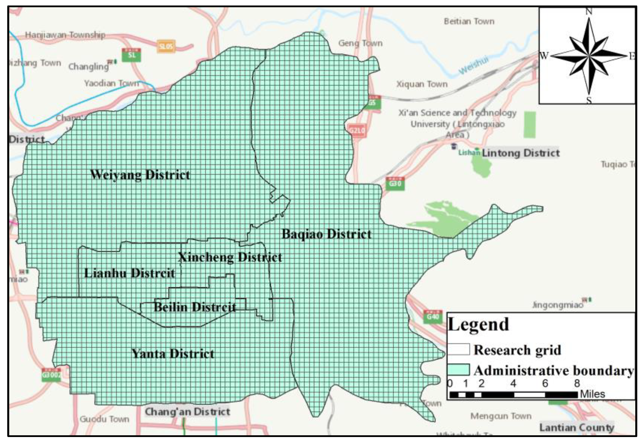
4.1. Study Area

Xi’an is an important central city in western China. Many studies have focused on the development of the taxi industry in Xi’an [58,59]. In addition, Xi’an has a long history of urban construction, and its road network has typical characteristics of ancient Chinese cities. Thus, Xi’an is a valuable experimental sample to analyze the relationship between taxi driver income and road network topology. At present, Xi’an has 11 municipal districts and 2 counties. Taxi pick-up and drop-off points are mainly located in the main urban area of Xi’an, and passengers generally do not take taxis when traveling to outer suburbs. In addition, the suburbs of Xi’an are in the transitional stage of urbanization, and the process of urban-rural integration needs to be further deepened. Therefore, we select the main urban area of Xi’an (Weiyang District, Xincheng District, Beilin District, Lianhu District, Baqiao district, and Yanta District) as the study area. Referring to the average street size in the main urban area of Xi’an [60], we adopt 400 m × 400 m grids as the analysis units, and divide the main urban area of Xi’an into 5079 grids. The study area and units are shown in Figure 1.

4.2. Data Source and Processing

The data source for this study comprises three parts: (1) taxi order data, sourced from Xi’an taxi management office; (2) urban POI data of Xi’an, obtained from Gaode Maps; (3) urban road network data, vectorized by the authors.

4.2.1. Taxi Order Data

Taxi order data used in this paper are provided by the Xi’an taxi management office. In the order data set, the pick-up and drop-off GPS points of multiple orders are recorded according to the time series (as described in Figure 2). In addition, the mileage and wait time of the process when drivers are searching for passengers are also detailed. The sample data format is shown in

Table 2. Taxi order data example.

Field	Sample	Unit	Meaning
car	***** 9H	/	License plate number
log_time	1 November 2019 9:50:53	/	Order information upload time
get_on_time	1 November 2019 9:33:00	/	Pick-up time
get_off_time	1 November 2019 9:51:00	/	Drop-off time
on_lon	108.927612	/	Longitude of pick-up points
on_lat	34.239687	/	Latitude of pick-up points
off_lon	108.939045	/	Longitude of drop-off points
off_lat	34.266075	/	Latitude of drop-off points
money	14.5	yuan	Order fee
mileage	4.9	km	Passenger mileage
free_mileage	1.3	km	Empty mileage
wait_time	360	s	Waiting time

. We selected the taxi order data of 20 working days and 20 non-working days from August to November of 2019 in Xi’an for analysis. During these working days and non-working days, there are no holidays and major events which may affect residents’ travel behaviors. The influence of holidays, special events, and the contingency of single day data on the research results is excluded. In the meantime, we eliminated invalid values, error values, and the values outside the research scope. What is more, the data whose order time is less than 1 min and more than 2 h are deleted. After the above steps, a total of approximately 12 million effective taxi order records are obtained.

Based on the taxi order records, we calculated the TOI, AOI, ADM, ADT, ASM, and AWT of taxi drivers in each grid on working days and non-working days. The formulas for calculation are as follows.

$$TO{I}_i={\displaystyle \sum _j^m{\displaystyle \sum _k^{n}O{I}_{ijk}}}$$

(11)

$$AO{I}_i=\frac{{\displaystyle \sum _j^m{\displaystyle \sum _k^{n}O{I}_{ijk}}}}{{\displaystyle \sum _j^m{\displaystyle \sum _k^n{O}_{ijk}}}}$$

(12)

$$AD{M}_i=\frac{{\displaystyle \sum _j^m{\displaystyle \sum _k^{n}D{M}_{ijk}}}}{{\displaystyle \sum _j^m{\displaystyle \sum _k^n{O}_{ijk}}}}$$

(13)

$$AD{T}_i=\frac{{\displaystyle \sum _j^m{\displaystyle \sum _k^{n}D{T}_{ijk}}}}{{\displaystyle \sum _j^m{\displaystyle \sum _k^n{O}_{ijk}}}}$$

(14)

$$AS{M}_i=\frac{{\displaystyle \sum _j^m{\displaystyle \sum _k^{n}S{M}_{ijk}}}}{{\displaystyle \sum _j^m{\displaystyle \sum _k^n{O}_{ijk}}}}$$

(15)

$$AW{T}_i=\frac{{\displaystyle \sum _j^m{\displaystyle \sum _k^{n}W{T}_{ijk}}}}{{\displaystyle \sum _j^m{\displaystyle \sum _k^n{O}_{ijk}}}}$$

(16)

where $TO{I}_i$ represents the total income of taxi orders whose origins are in grid $i$; $O{I}_{ijk}$ is the income from the order $j$ of taxi $k$ whose origin is in grid $i$; $AO{I}_i$ denotes the average income of taxi orders whose origins are in grid $i$; $O_{ijk}$ is the quantity of taxi orders whose origins are in grid $i$; $D{M}_{ijk}$ represents the delivery mileage of all taxi orders whose origins are in grid $i$; $AD{M}_{ijk}$ denotes the average delivery mileage of taxi orders whose origins are in grid $i$; $D{T}_{ijk}$ represents the duration time of all taxi orders whose origins are in grid $i$; $AD{T}_{ijk}$ denotes the average duration time of taxi orders whose origins are in grid $i$; $S{M}_{ijk}$ represents the search mileage of all taxi orders whose origins are in grid $i$; $AS{M}_{ijk}$ denotes the average search mileage of taxi orders whose origins are in grid $i$; $W{T}_{ijk}$ represents the waiting time of all taxi orders whose origins are in grid $i$; $AW{T}_{ijk}$ denotes the average waiting time of taxi orders whose origins are in grid $i$.

4.2.2. Urban POI Data

The point of interest (POI) data of Xi’an were collected from Gaode Maps. The eight attributes of POI data include: name, type, address, longitude coordinate, latitude coordinate, province, city, and district. The POI data used in this paper represent 13 types of urban function: catering service, scenic spot, public facility, shopping, traffic facility, education and culture, finance and insurance, commercial residence, life service, sports service, medical treatment service, government agency, and accommodation service. We measured the urban function mixing degree (UFMD) in different regions by calculating the spatial information entropy of urban function in each grid. It is defined as Equation (17).

$$E_{ij}=-{\displaystyle \sum _{i=1}^m{\displaystyle \sum _{j=1}^n\frac{A_{ij}^k}{A_{ij}}\times \log }}\frac{A_{ij}^k}{A_{ij}}$$

(17)

where $E_{ij}$ represents the spatial information entropy of urban function; $m$ is the number of rows in the study grids; $n$ is the number of columns in the study grids; $A_{ij}$ denotes the number of the total POIs; and $A_{ij}^k$ denotes the number of the POIs which belong to the category $k(k=1,2,3,\dots ,13)$ in the grid of row $i$ and column $j$.

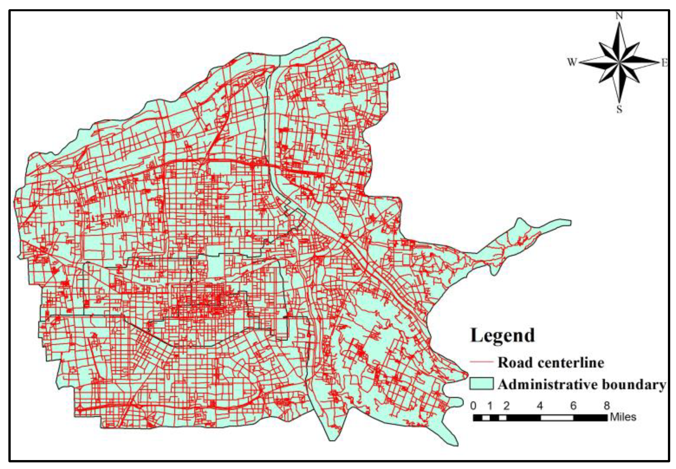
4.2.3. Urban Road Network Data

The line segment map is based on the road centerline, which has become the mainstream method for space syntax modeling and analysis. Compared with the axis model, it has a higher fitting degree for traffic flows [40]. Based on the Google online map, we vectorize the centerlines of the roads that taxis can pass through in the main urban area of Xi’an in ArcGIS 10.6 (excluding the internal roads in the closed areas such as communities, schools, units, etc.). A total of 14,041 road segments were obtained (as shown in Figure 3), and the road network line segment map of the main urban area of Xi’an was constructed after registration. The projected coordinate system of the shapefile is WGS 1984 Web Mercator Auxiliary Sphere, and the geographic coordinate system is GCS WGS 1984. Based on the line segment map, we calculate the closeness and betweenness of the road networks in the main urban area of Xi’an under different search radii with the Equations (1)–(3).

5. Results and Discussion

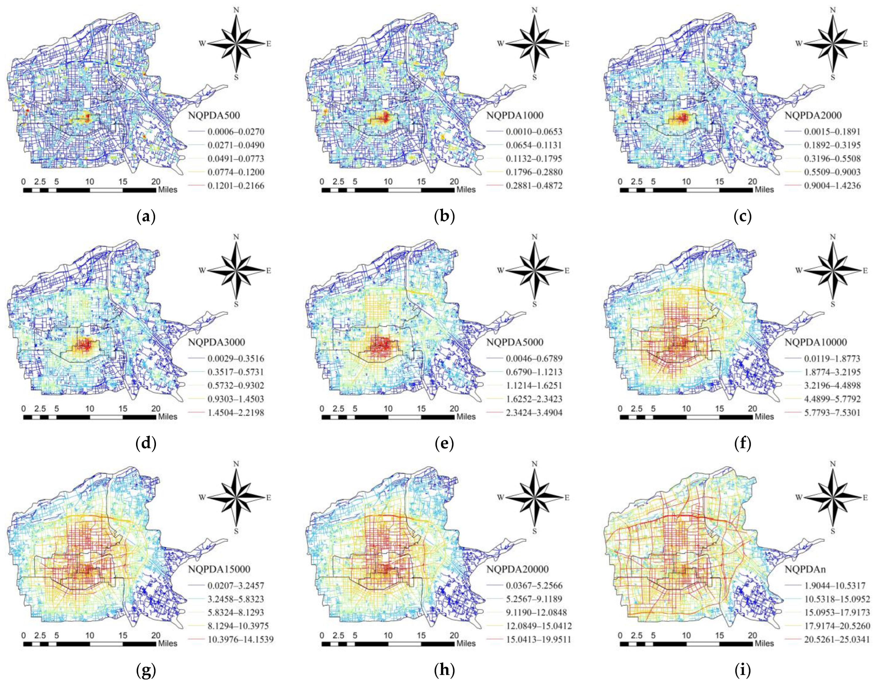
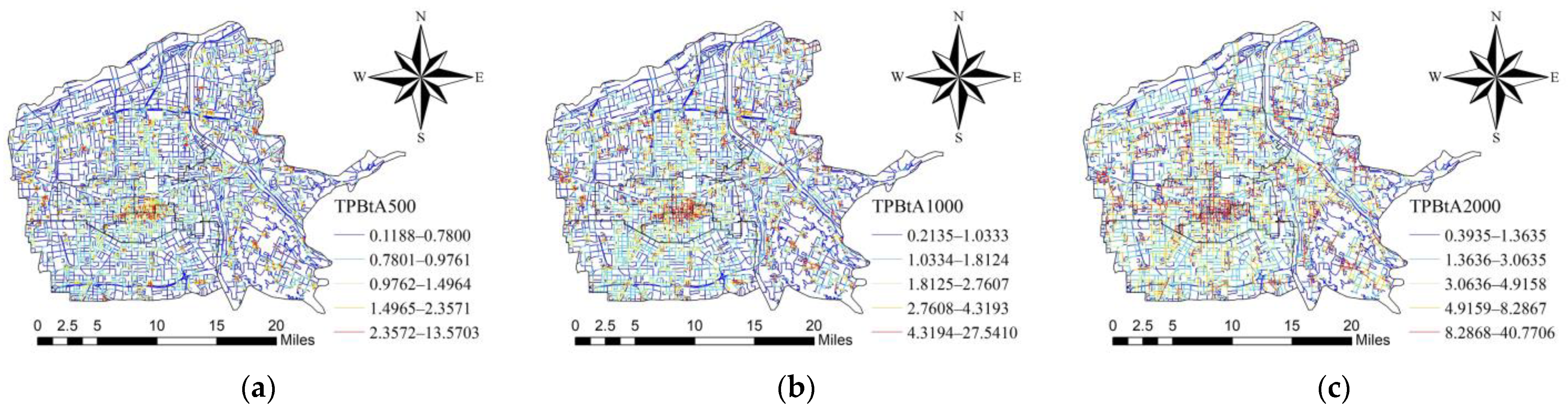
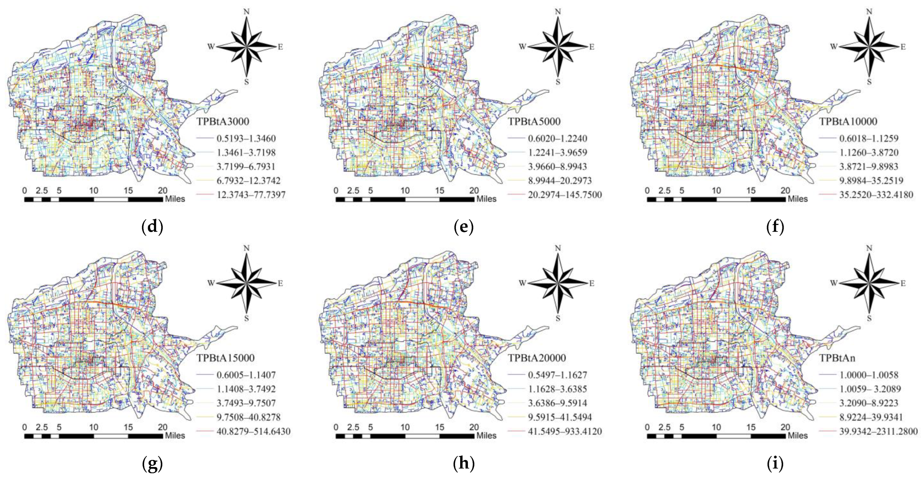
5.1. Analysis of Road Network Topological Characteristics in the Main Urban Area of Xi’an

In this paper, we analyzed the topological characteristics of the road networks in the main urban area of Xi’an under nine different search radii (500 m, 1000 m, 2000 m, 3000 m, 5000 m, 10,000 m, 15,000 m, 20,000 m, n). As shown in Figure 4 and Figure 5, the calculation results of urban road network topological indicators (closeness and betweenness) at different scales show different characteristics. Overall, the core area of closeness is the area within the city wall of Xi’an. With the expansion of the research scale, the high-value area of closeness gradually expands to the 3rd ring road and the ring expressway, and covers most of the main urban area of Xi’an. Under different research scales, the calculation results of closeness are more continuous and show a decreasing trend from the core area to the edge. At the research scales of 500 m, 1000 m, 2000 m, 3000 m, and 5000 m, the high-value area of closeness is mainly concentrated at the junction of Lianhu District, Xincheng District, and Beilin District (near the area within the city wall of Xi’an), where there are many business districts (Kaiyuan mall, Kangfu Road commercial circle, etc.). This indicates that closeness is closely related to the distribution of business districts. In the meantime, it also reflects the role of road network topology in shaping the urban commercial economy [61]. At the research scales of 10,000 m, 15,000 m, 20,000 m, and global scale, Weiyang District, Yanta District, and the area near the ring expressway in Baqiao District are gradually included in the high-value area of closeness. This shows that Lianhu District, Xincheng District, and Beilin District have strong attraction for short-distance and long-distance traffic flows, while Weiyang District, Yanta District, and Baqiao District lack attraction for short-distance traffic flows.

In contrast, the calculation results of betweenness in the main urban area of Xi’an do not show an obvious core region. With the expansion of the research scale, it gradually covers the main traffic roads in the research area. In general, the calculation results of betweenness are more discrete. To a certain extent, it has a uniform distribution of high-value sections and low-value sections. This phenomenon is related to the square format and circular distribution characteristics of traffic roads in the main urban area of Xi’an, which undertake a large number of passing traffic flows. At the research scales of 500 m, 1000 m, 2000 m, and 3000 m, the road networks at the junction of Lianhu District, Xincheng District, and Beilin District (near the area within the city wall of Xi’an) show the high-value area of betweenness. This phenomenon is related to the fact that there are many historical blocks in these places, which are suitable for short-distance slow traffic. At the research scales of 5000 m, 10,000 m, 15,000 m, 20,000 m, and the global scale, the main roads and transportation hubs in the main urban area of Xi’an are gradually included in the high-value area of betweenness, reflecting the basic characteristics of the main traffic roads within the research scope.

5.2. Spatial Correlation Analysis between Taxi Drivers’ Income and Road Network Topological Indicators

5.2.1. Global Spatial Correlation Analysis

By calculating the bivariate Moran’s I and relevant statistical indicators, we analyzed the global spatial correlation between the TOI of taxi drivers and road network topological indicators (closeness and betweenness) at different scales. As shown in

Table 3. Calculation results of bivariate Moran’s I between the TOI of taxi drivers and road network topological indicators.

Variables	Working Days			Non-Working Days
	Bivariate Moran’s I	Z-Score	Variance	Bivariate Moran’s I	Z-Score	Variance
NQPDA500	0.1383	17.9823	0.0077	0.1439	19.0352	0.0076
NQPDA1000	0.2011	24.3184	0.0083	0.2068	25.4641	0.0081
NQPDA2000	0.2810	34.0917	0.0082	0.2843	34.6012	0.0082
NQPDA3000	0.3240	37.4388	0.0086	0.3242	37.6663	0.0086
NQPDA5000	0.3650	41.3797	0.0088	0.3640	41.6306	0.0087
NQPDA10000	0.3535	41.0197	0.0086	0.3486	40.7272	0.0085
NQPDA15000	0.3253	38.7956	0.0084	0.3194	38.5672	0.0083
NQPDA20000	0.2982	36.3307	0.0082	0.2922	36.1358	0.0081
NQPDAn	0.1892	25.4042	0.0074	0.1832	25.3493	0.0072
TPBtA500	0.1210	15.9283	0.0076	0.1251	16.7538	0.0075
TPBtA1000	0.1338	18.1480	0.0074	0.1384	19.1481	0.0072
TPBtA2000	0.1437	18.1635	0.0079	0.1501	19.1999	0.0078
TPBtA3000	0.1280	16.3217	0.0078	0.1333	17.0148	0.0078
TPBtA5000	0.1181	15.5303	0.0075	0.1208	15.9730	0.0075
TPBtA10000	0.1091	15.2712	0.0071	0.1101	15.4915	0.0070
TPBtA15000	0.1063	14.3613	0.0073	0.1064	14.4561	0.0073
TPBtA20000	0.0921	12.1286	0.0075	0.0916	12.0858	0.0075
TPBtAn	0.0341	4.5490	0.0074	0.0340	4.5351	0.0074

, the results under all search radii passed the significance test at the 1% level. Overall, the TOI of taxi drivers has a certain degree of positive spatial correlation with closeness and betweenness under each research scale. Compared with betweenness, the positive spatial correlation between the TOI of taxi drivers and closeness is significantly higher under the same research scale. When the TOI of taxi drivers is the first variable and closeness is the second variable, the high values of bivariate Moran’s I mainly correspond to the search radii of smaller scales and medium scales (3000 m, 5000 m, 10,000 m, 15,000 m). In contrast, when betweenness is the second variable, the high values of bivariate Moran’s I only correspond to the search radii of smaller scales (500 m, 1000 m, 2000 m, 3000 m). In the meantime, whether the road network topological indicator is closeness or betweenness, the calculation results of bivariate Moran’s I are close under the same scale on working days and non-working days. This shows that the spatial correlation between the TOI of taxi drivers and road network topological indicators is rarely affected by the change in commuting traffic flows.

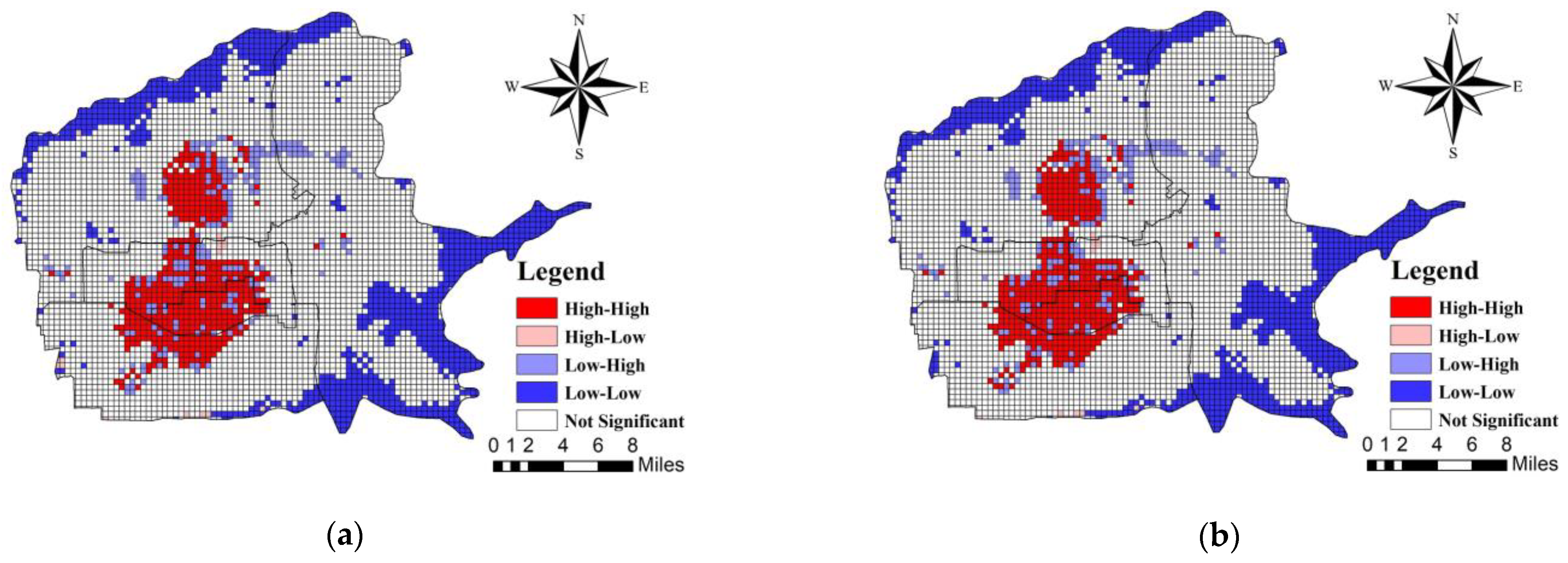
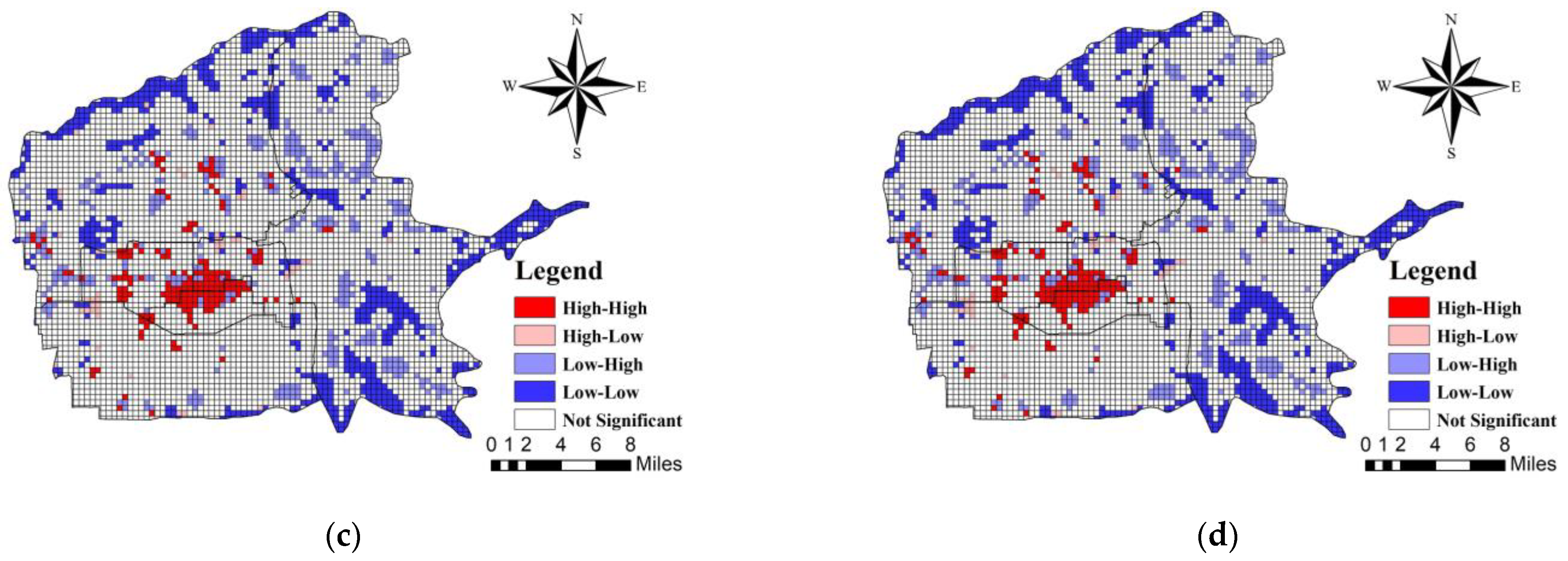
5.2.2. Local Spatial Correlation Analysis

Based on the road network topological indicators (NQPDA5000, TPBtA2000) corresponding to the maximum bivariate Moran’s I, we analyze the local spatial correlation between the TOI of taxi drivers and road network topological indicators on working days and non-working days. The LISA clustering results are shown in Figure 6 and reveal similar local spatial clustering and outlier characteristics under the same research scale on working days and non-working days. High-High (HH) indicates the spatial phenomenon in which research grids with high value of TOI are surrounded by research grids with high value of road network topological indicators; High-Low (HL) indicates the spatial phenomenon in which research grids with high value of TOI are surrounded by research grids with low value of road network topological indicators; Low-High (LH) indicates the spatial phenomenon in which research grids with low value of TOI are surrounded by research grids with high value of road network topological indicators; and Low-Low (LL) indicates the spatial phenomenon in which research grids with low value of TOI are surrounded by research grids with low value of road network topological indicators.

From the specific view, the TOI of taxi drivers and NQPDA5000 mainly presented HH and LL cluster states. HH regions are mainly located in Beilin District, Weiyang District, and the junction of Lianhu District, Xincheng District, Yanta District, and Beilin District, which covers the area within the city wall of Xi’an and the area along the subway line between Daminggong Station and Fengcheng 10th Road Station in Weiyang District. Such regions include the bustling business districts such as the Bell Tower business district in Beilin District, Xiaozhai business district in Yanta District, and Zhangjiabu business district in Weiyang District, where there are numerous shopping malls, entertainment facilities, office buildings, and catering facilities. In these regions, the demand for taxis is large, and the road networks are very accessible. Hence, it is easier for drivers to pick up passengers and earn more income. By comparison, LL regions are mainly located at the southeast of Baqiao District and the junction between the northwest of Weiyang District and Xianyang, which are suburban areas outside the ring expressway of Xi’an. As a matter of fact, the closeness of road networks in these regions is generally low and these regions lack attraction for traffic flows. Correspondingly, the demand for taxi travel is also significantly less, which leads to the phenomenon that taxi drivers’ income is low.

In contrast, the TOI of taxi drivers and TPBtA2000 mainly presented HH, LL, and LH cluster states. HH regions are mainly located in the junction of Lianhu District, Xincheng District, and Beilin District, where there are a lot of historical blocks, commercial streets, etc. In these regions, the demand for taxi travel is large, and the value of betweenness is high. Similar to the clustering characteristics of the TOI of taxi drivers and NQPDA5000, LL regions are also mainly located at the southeast of Baqiao District and the junction between the northwest of Weiyang District and Xianyang, which are suburban areas outside the ring expressway of Xi’an and have a lower value of betweenness. Notably, LH regions are basically distributed along the roads that bear a large number of passing traffic flows such as the ring expressway. Roads in this type of area have a higher betweenness, and there are fewer taxi stands. As a result, passengers are less likely to wait in such areas, and taxi drivers’ income is relatively lower.

5.3. Impact Analysis of Road Network Topological Variables on Taxi Drivers’ Income

5.3.1. Results of Multicollinearity Test

Table 4. The VIF of explanatory variables.

Date Category	Variable	Search Radius
		500 m	1000 m	2000 m	3000 m	5000 m	10,000 m	15,000 m	20,000 m	n
Working days	NQPDAR	7.3037	3.9471	2.6853	2.4257	2.2468	2.1802	2.0604	1.9193	1.4567
	TPBtAR	7.3743	3.7954	2.3601	1.9136	1.5389	1.3219	1.2570	1.2102	1.0967
	ADM	1.3818	1.3828	1.3852	1.3876	1.3918	1.3972	1.4004	1.4041	1.4135
	ADT	1.0841	1.0841	1.0839	1.0845	1.0851	1.0857	1.0845	1.0841	1.0838
	ASM	1.2734	1.2728	1.2714	1.2707	1.2695	1.2693	1.2688	1.2683	1.2695
	AWT	1.2319	1.2323	1.2330	1.2323	1.2320	1.2317	1.2320	1.2319	1.2316
	UFMD	1.2033	1.2754	1.3801	1.4899	1.6689	1.7911	1.7379	1.6455	1.3122
Non-working days	NQPDAR	7.3004	3.9447	2.6829	2.4280	2.2562	2.1996	2.0865	1.9411	1.4501
	TPBtAR	7.3572	3.7873	2.3539	1.9032	1.5292	1.3178	1.2561	1.2107	1.0965
	ADM	1.3036	1.3042	1.3064	1.3076	1.3126	1.3239	1.3296	1.3314	1.3292
	ADT	1.0837	1.0837	1.0837	1.0837	1.0838	1.0841	1.0844	1.0845	1.0845
	ASM	1.2619	1.2605	1.2604	1.2598	1.2601	1.2594	1.2592	1.2592	1.2597
	AWT	1.1125	1.1129	1.1123	1.1123	1.1124	1.1125	1.1130	1.1129	1.1126
	UFMD	1.2152	1.2865	1.3895	1.4976	1.6728	1.7901	1.7361	1.6434	1.3125

presents the VIF of all explanatory variables on working days and non-working days. The VIF of all variables is less than 10, which indicates that there is no obvious multicollinearity in the selected variables.

5.3.2. Results of Spatial Autocorrelation Test

Table 5. Spatial autocorrelation analysis results of explanatory variables.

Variable	Moran’s I	Z-Score	Variance	Variable	Moran’s I	Z-Score	Variance
NQPDA500	0.6638	65.4212	0.0001	TPBtA500	0.5453	53.7292	0.0001
NQPDA1000	0.7867	77.5360	0.0001	TPBtA1000	0.5786	57.0095	0.0001
NQPDA2000	0.8473	83.5191	0.0001	TPBtA2000	0.5836	57.5052	0.0001
NQPDA3000	0.8462	83.3921	0.0001	TPBtA3000	0.5327	52.5011	0.0001
NQPDA5000	0.8297	81.7309	0.0001	TPBtA5000	0.4474	44.1048	0.0001
NQPDA10000	0.8192	80.6863	0.0001	TPBtA10000	0.4075	40.1746	0.0001
NQPDA15000	0.8050	79.2863	0.0001	TPBtA15000	0.4160	41.0404	0.0001
NQPDA20000	0.7774	76.5718	0.0001	TPBtA20000	0.4233	41.8031	0.0001
NQPDAn	0.5867	57.8035	0.0001	TPBtAn	0.4153	41.1388	0.0001
ADM on working days	0.2259	23.1084	0.0001	ADM on non-working days	0.2412	23.8273	0.0001
ADT on working days	0.3496	34.4487	0.0001	ADT on non-working days	0.3651	35.9813	0.0001
ASM on working days	0.1553	15.4212	0.0001	ASM on non-working days	0.1391	13.9240	0.0001
AWT on working days	0.1012	10.1403	0.0001	AWT on non-working days	0.0448	6.4075	0.0001
UFMD	0.6888	67.8459	0.0001

reports the results of the Moran’s I test, which passed the significance test at the 1% level. The results indicate that significant spatial autocorrelation exists in all the explanatory variables and it is necessary to conduct the GWR model.

5.3.3. Model Comparison

We constructed OLS models and GWR models under nine research scales on working days and non-working days, respectively. In these models, the AOI of taxi drivers is the explained variable, and the explanatory variables include NQPDAR, TPBtAR, ADM, ADT, ASM, AWT, and UFMD (as shown in Table 1).

Table 6. Diagnostic information of OLS and GWR models.

Date Category	Search Radius	OLS			GWR
		R2	Adjusted R2	AICc	R2	Adjusted R2	AICc
Working days	500 m	0.987404	0.987387	−7785.938041	0.990464	0.990259	−9054.697923
	1000 m	0.987405	0.987388	−7786.242950	0.990428	0.990226	−9038.184838
	2000 m	0.987406	0.987389	−7786.676215	0.990297	0.99011	−8981.183506
	3000 m	0.987406	0.987389	−7786.785280	0.99025	0.99007	−8961.550904
	5000 m	0.987421	0.987404	−7792.839927	0.990219	0.990044	−8949.438457
	10,000 m	0.987478	0.987461	−7815.727285	0.990159	0.989992	−8924.594463
	15000 m	0.987535	0.987518	−7838.862552	0.990167	0.990002	−8930.625643
	20,000 m	0.987571	0.987554	−7853.553262	0.990212	0.990043	−8950.681031
	n	0.987573	0.987556	−7854.438004	0.990407	0.990209	−9030.502809
Non-working days	500 m	0.932685	0.932592	726.571381	0.948161	0.9475	−509.277002
	1000 m	0.932681	0.932588	726.857458	0.948048	0.947402	−500.405286
	2000 m	0.932710	0.932617	724.690041	0.948001	0.947364	−496.994085
	3000 m	0.932707	0.932614	724.907034	0.9479	0.947268	−488.04925
	5000 m	0.932706	0.932613	724.969798	0.947826	0.947198	−481.57563
	10,000 m	0.932745	0.932652	722.030340	0.947888	0.947267	−488.718107
	15,000 m	0.932803	0.932710	717.698034	0.9479	0.947285	−490.774212
	20,000 m	0.932812	0.932719	717.010204	0.947912	0.947296	−491.928945
	n	0.932797	0.932704	718.132490	0.947976	0.947327	−493.539596

presents the diagnostic information of the OLS and GWR models. Compared with the OLS models, it can be seen that the GWR models have the higher adjusted R² values. In addition, the AICc values of the GWR models are significantly lower than those of the OLS models, and the difference is greater than 3, which indicates that the GWR model is more suitable for the research content of this paper [62]. Therefore, we use the GWR model to analyze the impact of road network topological variables on taxi drivers’ income.

5.3.4. Analysis of Road Network Topological Variables Regression Results

Regression coefficient results for the road network topological variables are shown in

Table 7. Regression coefficient results of road network topological variables.

Date Category	Variable	Search Radius	Mean	Minimum	Maximum	Standard Deviation
Working days	Closeness	5000 m	−0.00431	−0.035486	0.018811	0.011366
		10,000 m	−0.008766	−0.035982	0.016315	0.013123
		15,000 m	−0.010014	−0.036503	0.011878	0.012304
		20,000 m	−0.009829	−0.034507	0.012109	0.011041
	Betweenness	10,000 m	0.002589	−0.005416	0.013602	0.004491
		15,000 m	0.002422	−0.004514	0.014182	0.00343
		20,000 m	0.002225	−0.005132	0.012993	0.003461
Non-working days	Closeness	10,000 m	−0.008884	−0.042869	0.014767	0.012282
		15,000 m	−0.010311	−0.043604	0.014635	0.011555
		20,000 m	−0.008081	−0.037731	0.018884	0.010344

, and the variables that failed the 1% significance test are not included. In general, closeness and betweenness have a significant impact on the AOI of taxi drivers at the medium and larger scales. However, their impact is not significant at the smaller scales, which indicates that the income of the taxi orders with short delivery distance is less affected by urban road network topology. During the working days, closeness has a significant negative impact on the AOI of taxi drivers. This impact increases with the increase of the search radius before 15,000 m, and decreases with the increase of the search radius after 15,000 m. Moreover, betweenness has a significant positive impact on the AOI of taxi drivers, which decreases with the increase of the search radius. Compared with betweenness, closeness has a greater impact on the AOI of taxi drivers. The reasons for these phenomena are complex. On the one hand, the road networks with a higher value of closeness have better topological integration and centrality, which have greater attraction for traffic flows. However, these road networks have higher road density, and there are a large number of vehicles and a higher possibility of congestion on these road networks. Therefore, residents near these road networks prefer to travel by public transport or select roads with more passing traffic flows to take taxis, so as to improve the success rate of hailing a taxi, as well as avoiding overly long waiting times and slower travel speeds. Moreover, previous studies also indicate that the areas with high-density road networks may act as a constraint on taxi trips [63,64], which is consistent with our findings above. As a result, the demand for taxis in the areas covered by these road networks has been restrained. On the other hand, it is easier for the traffic flows in the roads with a high value of closeness to reach the other parts of the road networks within the search radius. In addition, the urban functions in the areas covered by these road networks are highly mixed. Thus, it is more likely to form short-distance orders and short-time orders, which may result in less income from the same number of orders. In addition, previous research has shown that the high mixed degree of land use will lead to the emergence of short-distance taxi trips [65]. Moreover, the roads with a high value of betweenness are often urban expressways and arterial roads. Nearby passengers tend to take taxis on such roads, which increases the possibility of taking orders and helps taxi drivers earn higher income. On non-working days, closeness also has a significant negative impact on the AOI of taxi drivers, while betweenness has no significant impact on the AOI of taxi drivers. To a certain extent, it indicates that the impact of closeness on the AOI of taxi drivers is more stable, and it is less affected by the reduction of commuting traffic flows and the changes of the travel characteristics of residents during non-working days.

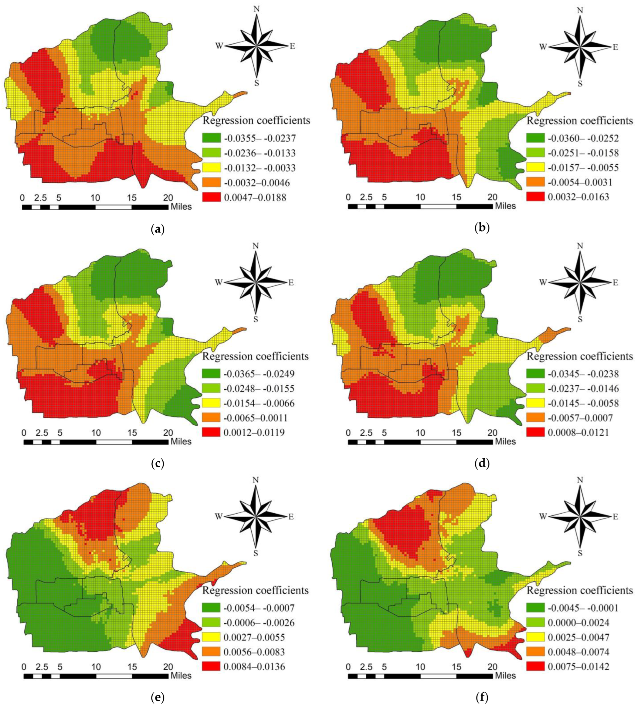
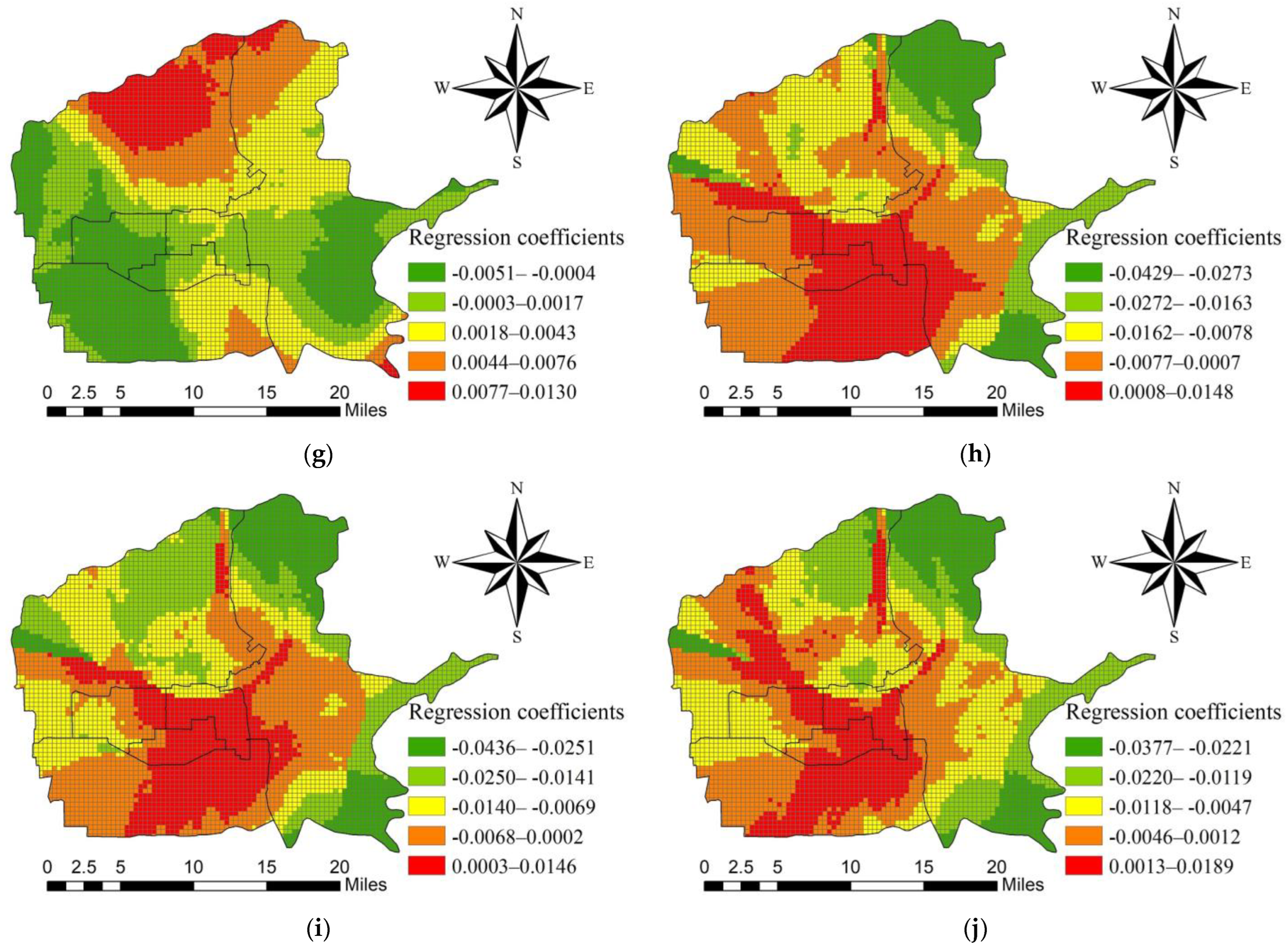
5.3.5. Spatial Pattern of Road Network Topological Variables Regression Coefficients

To analyze the spatial impact of road network topological variables, we use the natural break method to classify the local regression coefficients of road network topological variables which passed the 1% significance test. As shown in Figure 7, the spatial distribution of road network topological variables regression coefficients has some interesting characteristics. On the whole, regardless of working days or non-working days, the regression coefficients of road network topological variables show a certain degree of cross-scale similar characteristics. This indicates that the spatial impact of road network topology on the AOI of taxi drivers is stable. Specifically, on working days, the regression coefficient of closeness gradually increases from northeast to northwest, and southeast to southwest. The positive high-value area is mainly concentrated in the high-tech zone and the areas near Fengdong New City in the northwest of Weiyang District, while the negative high-value areas are located in the northern part of Weiyang District and the suburbs outside the ring expressway in Baqiao District. In fact, with the development of the high-tech zone and Fengdong New City, the closeness of the nearby road networks has been enhanced. At the same time, it also brings more jobs and travel demands, and promotes the increase of the AOI of taxi drivers. In contrast, the closeness of the road networks in the northern part of Weiyang District and the suburban areas outside the ring expressway in Baqiao District is lower. In these areas, taxis mainly travel on the roads with a higher value of betweenness. In the meantime, these areas are far from downtown, and the delivery distance of taxis in these areas is always long. Moreover, taxi drivers’ preference for passenger hot spots (such as the commercial area) also leads to a small number of total orders in these areas [1]. For these reasons, the AOI is relatively higher. In addition, in most areas, closeness and betweenness under the same scale have opposite impacts on the AOI of taxi drivers. Notably, the impact of closeness on the AOI of taxi drivers is greater than that of betweenness. This phenomenon indicates that the accessibility of road networks has a greater impact on taxi drivers’ income in comparison with the passing ability of road networks, and the opposite impact is often present in the same area. On non-working days, the high-value areas of regression coefficients of closeness are mainly distributed in Beilin District, Xincheng District, the east of Yanta District, and the areas within and near the city wall of Lianhu District, showing the decreasing characteristics from the high-value areas to the surroundings. Compared with working days, the regression coefficients of closeness on non-working days show the obvious spatial differentiation characteristics. The reasons are illustrated as follows. On the one hand, residents’ travel destinations and travel behavior characteristics are different on workdays and on non-working days. For instance, on non-working days, residents mainly travel for leisure, shopping, and entertainment by taxi. Thus, drivers may obtain higher AOI in the areas with more shopping malls, entertainment facilities, and catering facilities. In addition, most of these areas always have higher closeness. On the other hand, the changes in commuting traffic flows on urban roads also have an impact on the spatial distribution of taxi order income.

6. Conclusions

Taxi drivers’ income is an important topic in urban taxi research. Since taxis mainly travel on the road networks between different urban areas, taxi delivery activities and drivers’ income are closely related to the road network topological characteristics at different scales. However, previous studies have not focused on the impact of urban road network topology on taxi drivers’ income. In this paper, taking the main urban area of Xi’an as the research scope, we analyze the relationship between urban road network topology and taxi drivers’ income based on the method framework of sDNA, bivariate Moran’s I, and GWR. The major conclusions of this paper are summarized as follows.

(1)

The TOI of taxi drivers has a certain degree of positive spatial correlation with closeness and betweenness under each research scale. Compared with betweenness, the positive spatial correlation between the TOI of taxi drivers and closeness is significantly higher under the same research scale. This correlation shows little difference between working days and non-working days.

(2)

The impact of road network topological indicators at different scales on the AOI of taxi drivers is stable. Regardless of working days or non-working days, the impact of road network topological variables on the AOI of taxi drivers shows a certain degree of cross-scale similar features. Moreover, closeness and betweenness have a significant impact on the AOI of taxi drivers at the medium and larger scales.

(3)

As a whole, closeness has a negative impact on the AOI of taxi drivers, and betweenness has a positive impact on the AOI of taxi drivers. In most areas, closeness and betweenness under the same scale have opposite impacts on the AOI of taxi drivers. Compared with betweenness, the impact of closeness on the AOI of taxi drivers is greater and more stable.

These findings have important policy implications for urban managers and planners, and in particular, for the management of the taxi industry. Accordingly, urban taxi industry managers should pay more attention to the impact of road network topology on taxi drivers’ income and they should take road network factors into account when formulating policies such as vehicle allocation, price regulation, etc. Moreover, urban planners need to focus on the impact of road network topology on urban social economic phenomena when designing and optimizing road networks, so as to ensure the rationality of road network planning. Furthermore, taxi drivers can estimate the distribution of high-income areas and high-quality passengers based on the characteristics of the road networks in the operation area. In the process of searching for passengers, drivers should especially focus on the changes in the closeness of the nearby road networks to increase the possibility of obtaining higher-income orders. Furthermore, this paper focuses on urban road networks and taxi drivers’ income, and spans the gaps between urban road networks design, transport planning, and the urban taxi system. The methodological results obtained within this research work provide an evidence base for future researchers to explore the social and economic logic contained in the urban road network. In particular, the research framework of this paper can be extended to other travel modes, such as subways, BRT, private cars, and shared bikes.

Several limitations remain in this study. First, due to the lack of data, this paper has only examined the relationship between urban road network topology and the order income of cruising taxis. In the follow-up research, it is recommended that scholars take online car-hailing into consideration and further extend the results of this paper. Second, this study did not take into account the competitive relationship between taxis and other transportation modes, as well as the interaction of different traffic flows on the urban road networks. With that in mind, a number of possible future studies could further elucidate the precise influencing mechanism of road network topology on urban social economic phenomena. Last but not least, this study only focuses on the topological indicators near the pick-up locations of taxis. Further work needs to be conducted to investigate the impact of road network topology on taxi drivers’ income with different driving trajectories.

References

1. Zhang, D.; Sun, L.; Li, B.; Chen, C.; Pan, G.; Li, S.; Wu, Z. Understanding taxi service strategies from taxi GPS traces. IEEE Trans. Intell. Transp. Syst. 2014, 16, 123–135. [Google Scholar] [CrossRef]
2. Qin, G.; Li, T.; Yu, B.; Wang, Y.; Huang, Z.; Sun, J. Mining factors affecting taxi drivers’ incomes using GPS trajectories. Transp. Res. Part C Emerg. Technol. 2017, 79, 103–118. [Google Scholar] [CrossRef]
3. Ou, G.; Wu, Y.; Wang, G.; Guo, Z. Big-data-based analysis on the relationship between taxi travelling patterns and taxi drivers’ incomes. In Proceedings of the 2019 16th International Conference on Service Systems and Service Management (ICSSSM), Shenzhen, China, 13–15 July 2019; pp. 1–6. [Google Scholar]
4. Phiboonbanakit, T.; Horanont, T. How does taxi driver behavior impact their profit? Discerning the real driving from large scale GPS traces. In Proceedings of the 2016 ACM International Joint Conference on Pervasive and Ubiquitous Computing: Adjunct, Heidelberg, Germany, 12–16 September 2016; pp. 1390–1398. [Google Scholar]
5. Zhang, S.; Wang, Z. Inferring passenger denial behavior of taxi drivers from large-scale taxi traces. PLoS ONE 2016, 11, e0165597. [Google Scholar] [CrossRef]
6. Sun, L.; Zhang, D.; Chen, C.; Castro, P.S.; Li, S.; Wang, Z. Real time anomalous trajectory detection and analysis. Mob. Netw. Appl. 2013, 18, 341–356. [Google Scholar] [CrossRef]
7. Dong, Y.; Zhang, Z.; Fu, R.; Xie, N. Revealing New York taxi drivers’ operation patterns focusing on the revenue aspect. In Proceedings of the 2016 12th World Congress on Intelligent Control and Automation (WCICA), Guilin, China, 12–15 June 2016; pp. 1052–1057. [Google Scholar]
8. Liu, L.; Andris, C.; Ratti, C. Uncovering cabdrivers’ behavior patterns from their digital traces. Comput. Environ. Urban Syst. 2010, 34, 541–548. [Google Scholar] [CrossRef]
9. Tang, L.; Sun, F.; Kan, Z.; Ren, C.; Cheng, L. Uncovering distribution patterns of high performance taxis from big trace data. ISPRS Int. J. Geo-Inf. 2017, 6, 134. [Google Scholar] [CrossRef]
10. Ding, L.; Fan, H.; Meng, L. Understanding taxi driving behaviors from movement data. In AGILE 2015; Springer: Berlin/Heidelberg, Germany, 2015; pp. 219–234. [Google Scholar]
11. Naji, H.A.; Wu, C.; Zhang, H. Understanding the impact of human mobility patterns on taxi drivers’ profitability using clustering techniques: A case study in Wuhan, China. Information 2017, 8, 67. [Google Scholar] [CrossRef]
12. Gao, Y.; Xu, P.; Lu, L.; Liu, H.; Liu, S.; Qu, H. Visualization of taxi drivers’ income and mobility intelligence. In Proceedings of the International Symposium on Visual Computing, Rethymnon, Greece, 16–18 July 2012; pp. 275–284. [Google Scholar]
13. Kamga, C.; Yazici, M.A.; Singhal, A. Analysis of taxi demand and supply in New York City: Implications of recent taxi regulations. Transp. Plan. Technol. 2015, 38, 601–625. [Google Scholar] [CrossRef]
14. Yuan, C.; Wu, D.; Wei, D.; Liu, H. Modeling and analyzing taxi congestion premium in congested cities. J. Adv. Transp. 2017, 2017, 2619810. [Google Scholar] [CrossRef]
15. Yang, H.; Fung, C.; Wong, K.I.; Wong, S.C. Nonlinear pricing of taxi services. Transp. Res. Part A Policy Pract. 2010, 44, 337–348. [Google Scholar] [CrossRef]
16. Veloso, M.; Phithakkitnukoon, S.; Bento, C. Sensing urban mobility with taxi flow. In Proceedings of the 3rd ACM SIGSPATIAL International Workshop on Location-Based Social Networks, Chicago, IL, USA, 1 November 2011; pp. 41–44. [Google Scholar]
17. Sun, J.; Dong, H.; Qin, G.; Tian, Y. Quantifying the Impact of Rainfall on Taxi Hailing and Operation. J. Adv. Transp. 2020, 2020, 7081628. [Google Scholar] [CrossRef]
18. Wong, R.; Mak, P.; Szeto, W.; Yang, W. Spatio-temporal influence of extreme weather on a taxi market. Transp. Res. Rec. 2021, 2675, 639–651. [Google Scholar] [CrossRef]
19. Yu, J.; Xie, N.; Zhu, J.; Qian, Y.; Zheng, S.; Chen, X.M. Exploring impacts of COVID-19 on city-wide taxi and ride-sourcing markets: Evidence from Ningbo, China. Transp. Policy 2022, 115, 220–238. [Google Scholar] [CrossRef]
20. Putri, F.K.; Song, G.; Kwon, J.; Rao, P. DISPAQ: Distributed profitable-area query from big taxi trip data. Sensors 2017, 17, 2201. [Google Scholar] [CrossRef] [PubMed]
21. Devabhakthuni, K.; Munukurthi, B.; Rodda, S. Selection of Commercially Viable Areas for Taxi Drivers Using Big Data. In Smart Intelligent Computing and Applications; Springer: Berlin/Heidelberg, Germany, 2019; pp. 517–525. [Google Scholar]
22. Chen, Y.; Fu, Q.; Zhu, J. Finding next high-quality passenger based on spatio-temporal big data. In Proceedings of the 2020 IEEE 5th International Conference on Cloud Computing and Big Data Analytics (ICCCBDA), Chengdu, China, 10–13 April 2020; pp. 447–452. [Google Scholar]
23. Hu, B.; Zhang, S.; Ding, Y.; Zhang, M.; Dong, X.; Sun, H. Research on the coupling degree of regional taxi demand and social development from the perspective of job–housing travels. Phys. A Stat. Mech. Its Appl. 2021, 564, 125493. [Google Scholar] [CrossRef]
24. Chen, H.; Guo, B.; Yu, Z.; Wang, A.; Zheng, C. The Framework of Increasing Drivers’ Income on the Online Taxi Platforms. IEEE Trans. Netw. Sci. Eng. 2020, 7, 2182–2191. [Google Scholar] [CrossRef]
25. Qu, B.; Yang, W.; Cui, G.; Wang, X. Profitable taxi travel route recommendation based on big taxi trajectory data. IEEE Trans. Netw. Sci. Eng. 2019, 21, 653–668. [Google Scholar] [CrossRef]
26. Qiu, Y.; Xu, X. RPSBPT: A route planning scheme with best profit for taxi. In Proceedings of the 2018 14th International Conference on Mobile Ad-Hoc and Sensor Networks (MSN), Hefei, China, 6–8 December 2018; pp. 121–126. [Google Scholar]
27. Zhang, D.; Zhou, C.; Sun, D.; Qian, Y. The influence of the spatial pattern of urban road networks on the quality of business environments: The case of Dalian City. Environ. Dev. Sustain. 2021, 24, 9429–9446. [Google Scholar] [CrossRef]
28. Said, M.; Geha, G.; Abou-Zeid, M. Natural experiment to assess the impacts of street-level urban design interventions on walkability and business activity. Transp. Res. Rec. 2020, 2674, 258–271. [Google Scholar] [CrossRef]
29. Matthews, J.W.; Turnbull, G.K. Neighborhood street layout and property value: The interaction of accessibility and land use mix. J. Real Estate Financ. Econ. 2007, 35, 111–141. [Google Scholar] [CrossRef]
30. Yoshimura, Y.; Santi, P.; Arias, J.M.; Zheng, S.; Ratti, C. Spatial clustering: Influence of urban street networks on retail sales volumes. Environ. Plan. B Urban Anal. City Sci. 2021, 48, 1926–1942. [Google Scholar] [CrossRef]
31. Xiao, Y.; Orford, S.; Webster, C.J. Urban configuration, accessibility, and property prices: A case study of Cardiff, Wales. Environ. Plan. B Plan. Des. 2016, 43, 108–129. [Google Scholar] [CrossRef]
32. Batty, M. Accessibility: In search of a unified theory. Environ. Plan. B Plan. Des. 2009, 36, 191–194. [Google Scholar] [CrossRef]
33. Porta, S.; Latora, V.; Wang, F.; Rueda, S.; Strano, E.; Scellato, S.; Cardillo, A.; Belli, E.; Cardenas, F.; Cormenzana, B. Street centrality and the location of economic activities in Barcelona. Urban Stud. 2012, 49, 1471–1488. [Google Scholar] [CrossRef]
34. Merchan, D.; Winkenbach, M.; Snoeck, A. Quantifying the impact of urban road networks on the efficiency of local trips. Transp. Res. Part A Policy Pract. 2020, 135, 38–62. [Google Scholar] [CrossRef]
35. Wang, S.; Yu, D.; Kwan, M.-P.; Zheng, L.; Miao, H.; Li, Y. The impacts of road network density on motor vehicle travel: An empirical study of Chinese cities based on network theory. Transp. Res. Part A Policy Pract. 2020, 132, 144–156. [Google Scholar] [CrossRef]
36. Koohsari, M.J.; Owen, N.; Cole, R.; Mavoa, S.; Oka, K.; Hanibuchi, T.; Sugiyama, T. Built environmental factors and adults’ travel behaviors: Role of street layout and local destinations. Prev. Med. 2017, 96, 124–128. [Google Scholar] [CrossRef]
37. Orellana, D.; Guerrero, M.L. Exploring the influence of road network structure on the spatial behaviour of cyclists using crowdsourced data. Environ. Plan. B Urban Anal. City Sci. 2019, 46, 1314–1330. [Google Scholar] [CrossRef]
38. Zlatkovic, M.; Zlatkovic, S.; Sullivan, T.; Bjornstad, J.; Shahandashti, S.K.F. Assessment of effects of street connectivity on traffic performance and sustainability within communities and neighborhoods through traffic simulation. Sustain. Cities Soc. 2019, 46, 101409. [Google Scholar] [CrossRef]
39. Choi, D.-A.; Ewing, R. Effect of street network design on traffic congestion and traffic safety. J. Transp. Geogr. 2021, 96, 103200. [Google Scholar] [CrossRef]
40. Serok, N.; Levy, O.; Havlin, S.; Blumenfeld-Lieberthal, E. Unveiling the inter-relations between the urban streets network and its dynamic traffic flows: Planning implication. Environ. Plan. B Urban Anal. City Sci. 2019, 46, 1362–1376. [Google Scholar] [CrossRef]
41. Hillier, B.; Iida, S. Network and psychological effects in urban movement. In Proceedings of the International Conference on Spatial Information Theory, Ellicottville, NY, USA, 14–18 September 2005; pp. 475–490. [Google Scholar]
42. Hillier, B.; Hanson, J. The Social Logic of Space; Cambridge University Press: Cambridge, UK, 1989. [Google Scholar]
43. Hillier, B. Space Is the Machine: A Configurational Theory of Architecture; Space Syntax: London, UK, 2007. [Google Scholar]
44. Hillier, B.; Penn, A.; Hanson, J.; Grajewski, T.; Xu, J. Natural movement: Or, configuration and attraction in urban pedestrian movement. Environ. Plan. B Plan. Des. 1993, 20, 29–66. [Google Scholar] [CrossRef]
45. Hillier, W.; Yang, T.; Turner, A. Normalising least angle choice in Depthmap-and how it opens up new perspectives on the global and local analysis of city space. J. Space Syntax 2012, 3, 155–193. [Google Scholar]
46. Cooper, C.H.; Chiaradia, A.J. sDNA: 3-d spatial network analysis for GIS, CAD, Command Line & Python. SoftwareX 2020, 12, 100525. [Google Scholar] [CrossRef]
47. Powell, J.W.; Huang, Y.; Bastani, F.; Ji, M. Towards reducing taxicab cruising time using spatio-temporal profitability maps. In Proceedings of the International Symposium on Spatial and Temporal Databases, Minneapolis, MN, USA, 24–26 August 2011; pp. 242–260. [Google Scholar]
48. Ding, Y.; Liu, S.; Pu, J.; Ni, L.M. Hunts: A trajectory recommendation system for effective and efficient hunting of taxi passengers. In Proceedings of the 2013 IEEE 14th International Conference on Mobile Data Management, Milan, Italy, 3–6 June 2013; pp. 107–116. [Google Scholar]
49. Huang, H.; Fang, Z.; Wang, Y.; Tang, J.; Fu, X. Analysing taxi customer-search behaviour using Copula-based joint model. Transp. Saf. Environ. 2022, 4, tdab033. [Google Scholar] [CrossRef]
50. Yuan, N.J.; Zheng, Y.; Zhang, L.; Xie, X. T-finder: A recommender system for finding passengers and vacant taxis. IEEE Trans. Knowl. Data Eng. 2012, 25, 2390–2403. [Google Scholar] [CrossRef]
51. Li, X.; Sun, Y.-E.; Liu, Q.; Shen, Z.; Song, B.; Du, Y.; Huang, H. PROMISE: A taxi recommender system based on inter-regional passenger mobility. In Proceedings of the 2019 International Joint Conference on Neural Networks (IJCNN), Budapest, Hungary, 14–19 July 2019; pp. 1–8. [Google Scholar]
52. Wang, H.; Rong, H.; Zhang, Q.; Liu, D.; Hu, C.; Hu, Y. Good or Mediocre? A Deep Reinforcement Learning Approach for Taxi Revenue Efficiency Optimization. IEEE Trans. Netw. Sci. Eng. 2020, 7, 3018–3027. [Google Scholar] [CrossRef]
53. Gao, Y.; Jiang, D.; Xu, Y. Optimize taxi driving strategies based on reinforcement learning. Int. J. Geogr. Inf. Sci. 2018, 32, 1677–1696. [Google Scholar] [CrossRef]
54. Zhou, X.; Rong, H.; Yang, C.; Zhang, Q.; Khezerlou, A.V.; Zheng, H.; Shafiq, Z.; Liu, A.X. Optimizing taxi driver profit efficiency: A spatial network-based markov decision process approach. IEEE Trans. Big Data 2018, 6, 145–158. [Google Scholar] [CrossRef]
55. Chiaradia, A.J.; Cooper, C.; Webster, C. Spatial Design Network Analysis Software. 2013. Available online: http://www.cardiff.ac.uk/sdna/ (accessed on 17 June 2022).
56. Zhang, Y.; Liu, Y.; Zhang, Y.; Liu, Y.; Zhang, G.; Chen, Y. On the spatial relationship between ecosystem services and urbanization: A case study in Wuhan, China. Sci. Total Environ. 2018, 637, 780–790. [Google Scholar] [CrossRef]
57. Fotheringham, A.S. Trends in quantitative methods I: Stressing the local. Prog. Hum. Geogr. 1997, 21, 88–96. [Google Scholar] [CrossRef]
58. Liu, Z.; Chen, H.; Li, Y.; Zhang, Q. Taxi demand prediction based on a combination forecasting model in hotspots. J. Adv. Transp. 2020, 2020, 1302586. [Google Scholar] [CrossRef]
59. Yang, Y.; He, Z.; Song, Z.; Fu, X.; Wang, J. Investigation on structural and spatial characteristics of taxi trip trajectory network in Xi’an, China. Phys. A Stat. Mech. Its Appl. 2018, 506, 755–766. [Google Scholar] [CrossRef]
60. Research Institute for Road Safety of MPS; Cennavi; China Academy of Urban Planning & Design. Portrait Report on the Road Network Structure of China’s Key Cities; 2020. Available online: https://baijiahao.baidu.com/s?id=1685489050502555860&wfr=spider&for=pc (accessed on 21 June 2022).
61. Ni, J.; Qian, T.; Xi, C.; Rui, Y.; Wang, J. Spatial distribution characteristics of healthcare facilities in Nanjing: Network point pattern analysis and correlation analysis. Int. J. Environ. Res. Public Health 2016, 13, 833. [Google Scholar] [CrossRef]
62. Fotheringham, A.S.; Brunsdon, C.; Charlton, M. Geographically Weighted Regression: The Analysis of Spatially Varying Relationships; John Wiley & Sons: New York, NY, USA, 2003. [Google Scholar]
63. Zhang, X.; Huang, B.; Zhu, S. Spatiotemporal influence of urban environment on taxi ridership using geographically and temporally weighted regression. ISPRS Int. J. Geo-Inf. 2019, 8, 23. [Google Scholar] [CrossRef]
64. Qian, X.; Ukkusuri, S.V. Spatial variation of the urban taxi ridership using GPS data. Appl. Geogr. 2015, 59, 31–42. [Google Scholar] [CrossRef]
65. Cervero, R.; Kockelman, K. Travel demand and the 3Ds: Density, diversity, and design. Transp. Res. Part D Transp. Environ. 1997, 2, 199–219. [Google Scholar] [CrossRef]
Figure 1. Study area and units.
Ijgi 11 00464 g001
Figure 2. Description of taxi order data.
Ijgi 11 00464 g002
Figure 3. The road network line segment map of the main urban area of Xi’an.
Ijgi 11 00464 g003
Figure 4. The closeness of the road networks at different scales in the main urban area of Xi’an (R denotes search radius). (a) R = 500 m; (b) R = 1000 m; (c) R = 2000 m; (d) R = 3000 m; (e) R = 5000 m; (f) R = 10,000 m; (g) R = 15,000 m; (h) R = 20,000 m; (i) R = n.
Ijgi 11 00464 g004
Figure 5. The betweenness of the road networks at different scales in the main urban area of Xi’an (R denotes search radius). (a) R = 500 m; (b) R = 1000 m; (c) R = 2000 m; (d) R = 3000 m; (e) R = 5000 m; (f) R = 10,000 m; (g) R = 15,000 m; (h) R = 20,000 m; (i) R = n.
Ijgi 11 00464 g005aIjgi 11 00464 g005b
Figure 6. Bivariate local Moran’s I analysis map. (a) The TOI of taxi drivers is the first variable and NQPDA5000 is the second variable on working days. (b) The TOI of taxi drivers is the first variable and NQPDA5000 is the second variable on non-working days. (c) The TOI of taxi drivers is the first variable and TPBtA2000 is the second variable on working days. (d) The TOI of taxi drivers is the first variable and TPBtA2000 is the second variable on non-working days.
Ijgi 11 00464 g006aIjgi 11 00464 g006b
Figure 7. Spatial patterns of road network topological variables regression coefficients. (a) NQPDA5000, working days; (b) NQPDA10000, working days; (c) NQPDA15000, working days; (d) NQPDA20000, working days; (e) TPBtA10000, working days; (f) TPBtA15000, working days; (g) TPBtA20000, working days; (h) NQPDA10000, non-working days; (i) NQPDA15000, non-working days; (j) NQPDA20000, non-working days.
Ijgi 11 00464 g007aIjgi 11 00464 g007b