Article

Explore the Correlation between Environmental Factors and the Spatial Distribution of Property Crime

1
Chinese Academy of Surveying and Mapping, Beijing 100830, China
2
School of Earth Science and Resources, Chang’an University, Xi’an 710054, China
3
School of Geography and Environment Science, Tianjin Normal University, Tianjin 300387, China
4
School of Economics and Management, Beijing University of Technology, Beijing 100124, China
5
College of Resource and Environmental Science, Wuhan University, Wuhan 430072, China
*
Author to whom correspondence should be addressed.
ISPRS Int. J. Geo-Inf. 2022, 11(8), 428; https://doi.org/10.3390/ijgi11080428
Submission received: 26 May 2022 / Revised: 22 July 2022 / Accepted: 25 July 2022 / Published: 28 July 2022

Abstract

:
Comprehensively understanding the factors influencing crime is a prerequisite for preventing and combating crime. Although some studies have investigated the relationship between environmental factors and property crime, the interaction between factors was not fully considered in these studies, and the explanation of complex factors may be insufficient. This paper explored the influence of environmental factors on property crime using factor regression and factor interaction based on data from the central city of Lanzhou, China. Our findings showed that: (1) The distribution of crime cases showed the pattern of a local multi-center. Shop density, hotel density, entertainment density and house price were the four dominant environmental drivers of property crime; (2) The relationship between the light intensity and property crime had different correlation explanations in temporal projection and spatial projection. There was a normal distribution curve between the number of property crimes and the Price-to-Earnings Ratio (PE Ratio) of the community house price; and (3) The results of the factor interaction indicated that the effect of all factors on crime showed a two-factor enhancement. As an important catalyst, shop density had the strongest interaction with other factors. Shop density gradient influenced the degree of interpretation of spatial heterogeneity of property crime.

1. Introduction

Crime poses a major threat to urban areas in many countries. This is because it not only results in injury and property loss, but also increases the general fear of crime and feelings of insecurity [1]. Property offences are commonly considered less serious than personal crimes. Nonetheless, they significantly affect individual victims and negatively influence the overall quality of urban life. Across all crime categories, property crimes such as burglary, larceny and motor vehicle theft and sometimes robbery are generally the most frequent individual offences, with a ratio that usually far exceeds either violent crimes or other types of crime. Among all property crimes, burglary is probably the most invasive offence, often carrying with it a long-term psychological impact on victims, stigma for neighborhoods and districts, and implications for planning and design. Robbery is a major security threat and a special concern in developing countries. Property crime accounted for the largest share of total crimes in China [2], accounting for 30.3% of all reported crime cases from 2013 to 2017.
Geographical environment has always played an important role in affecting criminal activities as it is the sphere of direct interaction between nature and society. In the 18th century, “classical criminological theories” were developed on the basis of Enlightenment ideas [3]. The Chicago School of Criminology was identified with social neighborhood space studies of crime and delinquency that focus particularly on the spatial patterns of such behavior, especially as reflected in maps of their spatial distributions, and proposed social structure theories [4]—Social Disorganization Theory [5], Differential Association Theory [6] and Social Learning Theory [7]—which represent a group of so-called positivist approaches to crime research that took shape in the nineteenth century. It was a reflection of the belief that only scientific methods of explanation would help to elucidate the causes of criminal behavior. Belton Fileisher [8] and Gary Becker [9] have previously suggested that crime may be explainable. In the 1960s and 1970s, humanism and positivism further promoted the cognition and understanding of the space of individuals in crime research. The layout and design of urban living environment was considered to be an important factor affecting some regions prone to criminal behavior. During this period, theories such as crime prevention through environmental design (CPTED) [10], defensible space theory [10] and situational crime prevention [11] emerged successively. Matlovicova K. et al. used the example of Slovak cities to show that crime prevention or its reduction were possible through urban environment formation and modification [3,12,13]. Since the late 1980s, a solid theoretical background about the spatial and temporal dimensions of crime has been established [14,15,16], including well-known theories such as routine activity [17], rational choice [18] and geometry of crime [19] and supports the understanding of the crime mechanism, which is a crucial initial step toward crime reduction [20,21]. These models have added insights that help in the understanding of crime offences. Some studies have proved that there is a certain relationship between environmental factors and the occurrence of crime. For example, Ceccato [22] found that thefts and robberies in São Paulo, Brazil, were concentrated around subway stations in the center of the city. Liu et al. [23] explored the influence of changes in the location of bus stops on street robberies in Cincinnati. Hipp J.R. studied the effect of housing age and housing type on crime at different spatial scales [24]. Boivin discussed the relationship between population density and crime rate in Toronto [25]. The results showed that the relationship between population density and crime rate was uncertain in different scenarios, and it might increase or decrease. Some studies have shown that dark environments were conducive to crime, and crime rates have dropped significantly in areas with improved street lighting [26,27]. In promoting community pride and informal social control, street lighting seemed to be more useful than strengthening surveillance and deterrence. However, some scholars believed that the lighting in some hidden areas could not only improve the street visibility of pedestrians, but also improve the visibility of criminals, which may help them choose the target of the crime and escape after committing the crime [28]. At present, crime research has continued to focus on reducing situational opportunity to carry out crime by changing the environment, which benefited from the application of GIS and spatial statistics in studying regional crime, as well as the addition of architecture, urban planning and design and other disciplines. The environmental factors about the crime space obtained from various data sources are more and more complex and closer to the real urban environment. Since there are many environmental factors affecting crime, we would like to know the difference in the interpretation of multiple environmental factors on crime and the interpretation of interactive environmental factors on crime; after all, the criminal environment is not composed of a single factor, but instead of complexity.
The purpose of this study is not to delve into the mechanism of these models but to explore the environmental variables on the spatial distribution of property crime to increase our understanding of the complexity of property crime across space. Regression models are of utmost importance to both law enforcement agencies and academic research [29]. Based on ordinary least squares regression and geographically weighted regression, Cabrera-Barona analyzed the relationship between crime types and poverty, population density and police in the metropolitan area [30]. Michelle Kondo studied the influence of green space and community vacant land on crime by using linear regression and Poisson regression model [31]. Cundiff used multilevel negative binomial regression to analyze the relationship between college campuses and violent and property crime rates [32]. The results showed that the closer to the campus, the higher the crime rate, after controlling for other community and city-level indicators. Although the regression model can independently show the influence degree of factors on geographical phenomena, it does not fully consider the interaction between factors, and the explanation of complex factors may be insufficient. Crime is a complex social behavior, and its occurrence is the result of the joint action of social, individual, natural and other environmental factors. Interaction between factors can inherently be attributed to the coupling mechanism between different theories. For example, the social disorganization theory could interpret the criminal motivation in routine activity theory in some cases, while the lack of supervision in routine activity theory may interpret the effect of social conflicts in social disorganization theory. Compared with regression analysis, the Geo-detector takes into account the interaction between factors. It reveals the driving forces of geographical phenomena by detecting their spatial stratified heterogeneity (SSH), which means it is an effective and suitable method to explain the complex drivers of crime. Although the Geo-detector can effectively detect the influence of factor interaction on geographical phenomena, it cannot determine the positive or negative correlations of independent factors and lacks the ability of regression models to simulate the characteristics of the dependent variables. At present, there is poor understanding and few studies of combined factors of regression and interaction to explore the factors influencing property crime. Therefore, this paper explored and measured the interpretation of multiple factors on the spatial density of property crime in the study area by combining factor regression and interaction through the collection of environmental factors.

2. Materials and Methods
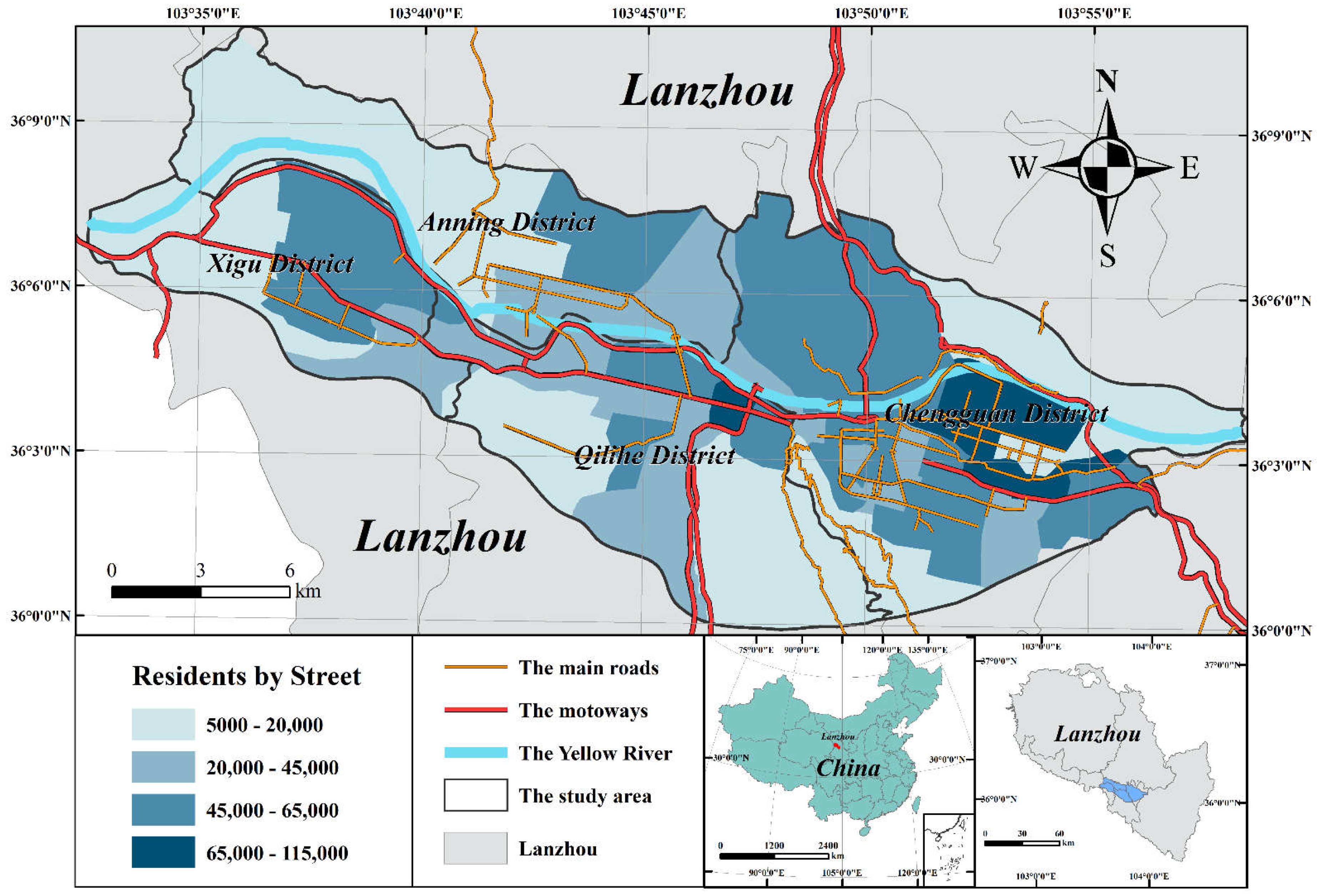
2.1. The Case Study

Lanzhou is a significant commercial center and comprehensive transportation hub in northwest China with a long history, and it is also an important city in the Silk Road Eco-nomic Belt and an important inflow place for floating population in Northwest China. It has 5 districts and 3 counties under its jurisdiction, with a total area of 13,100 square kilometers and a resident population of about 4.38 million. Lanzhou is a multi-ethnic city with 56 ethnic groups, in which the most crowded group is the Han, accounting for 95.88% of the city’s population. Most of the people live in the central urban area, the Chengguan District, Xigu District, Anning District and Qilihe District (Figure 1). The central urban area accounts for only 2.75% of the city’s area, but it concentrates 67.70% of the city’s population, with an average population density of 2716 person/km2, and is a high population density area. As an important central city in northwest China, Lanzhou has attracted a large number of floating migrants. The influx of population not only provides cheap labor for urban construction, but the high-density population agglomeration also brings some pressure to the public security management of the city. Thus, the selection of Lanzhou central city as the study area for property crime driving factors has an important social significance.

2.2. Data Sources and Preprocessing
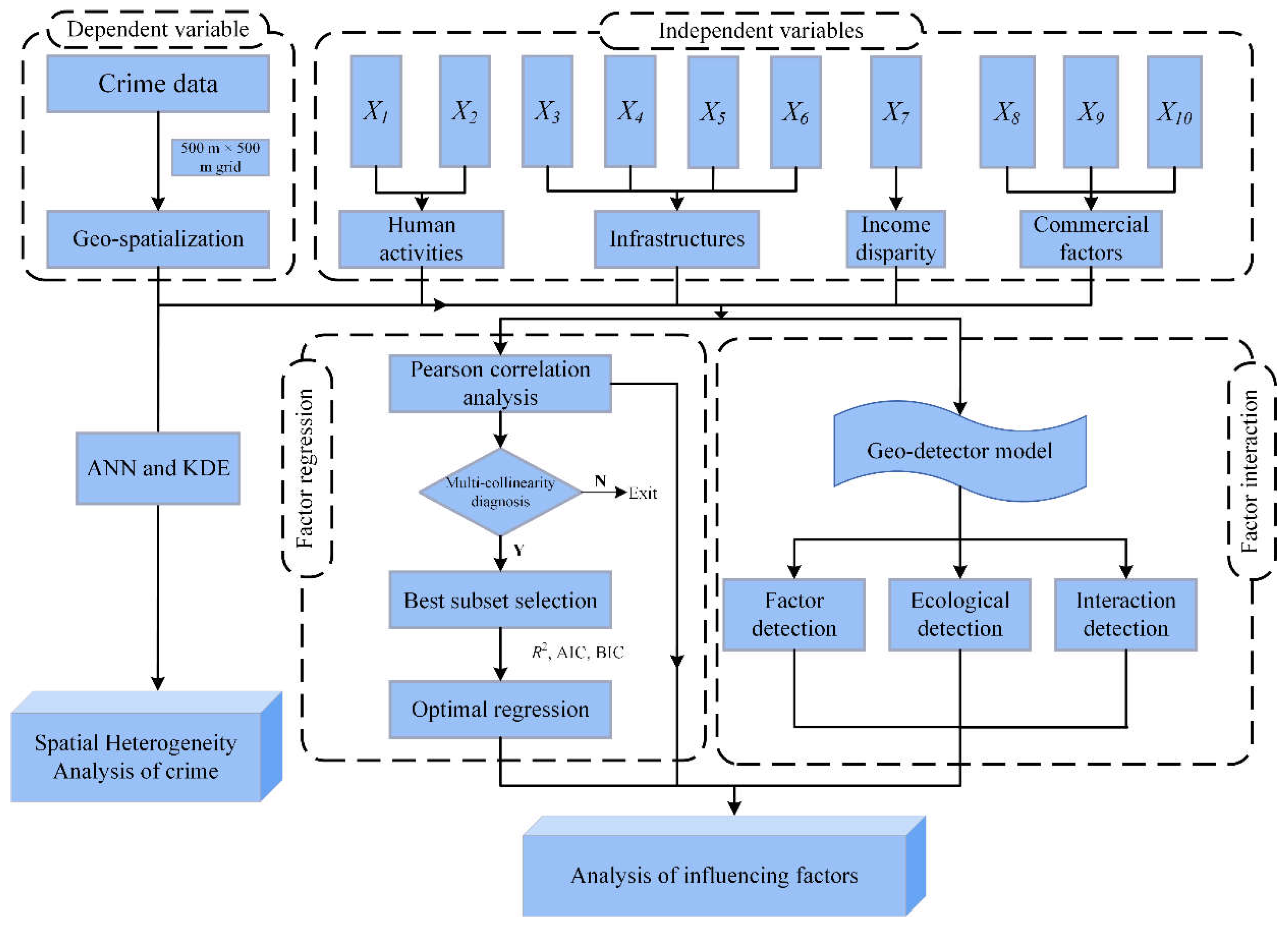
We collected data for property crimes (including burglary, larceny, motor vehicle theft and robbery) and their environmental influencing factors from multiple sources. The records of property crime were used as the dependent variable to analyze the spatial heterogeneity. This dataset was free downloaded from China Judgements Online [33], including the time, the place and the category of crime. It has been widely used and proven to be effective in reflecting the spatial pattern of urban crime in China [34,35,36]. We extracted a total of 2207 property crime records that occurred in the central urban area of Lanzhou from 2014 to 2016, and they were geo-graphically coded to determine the spatial location.
Considering the complexity of the crime conditions, a frameset including 10 representative variables factors was designed from human activity, socio-economic and infrastructure as potential risk factors to analyze the effect of these factors on property crime (see Figure 2 and Table 1). Population density and night lighting represent the intensity of human activity [37,38]. The density of the road network, the distance to the police stations, the distance to the main roads and the distance to the bus stops represent the perfect degree of infrastructure and traffic accessibility [24,39,40,41]. To some extent, the average house price is related to the local income level, and the gap in income levels will aggravate crime [42,43]. Entertainment density, hotel density and shop density reflect the business environment, and there may be more potential victims in more prosperous areas [44,45,46,47], and they were also introduced as independent variables.
The population data were obtained from the community population survey by the Lanzhou Municipal Public Security Bureau. The night light data with the 500 m × 500 m resolution came from NPP-VIIRS [48]. Considering that the shading effect of vegetation canopy in winter is weaker than in other seasons, nightlight images in winter can detect the urban environment more clearly [49], the synthetic image data in 2016 was selected. The image eliminated the light saturation effect, improved the signal-to-noise ratio and eliminated obvious noise. In the study, the image was reclassified in order to facilitate analysis, and the range of pixel value is 0–400. The road network data came from OpenStreetMap [50], and was obtained after pre-processing such as topological rules check, editing and modifications based on geographic national conditions monitoring data in Lanzhou. The house price data were downloaded from the “Anjuke” website [51]. After data cleaning and spatialization, the average house price records of 2661 communities in the main urban area of Lanzhou in 2016 were obtained. The POI data including police stations, bus stops, entertainment venues, hotels and shops were derived from the Amap [52]. They were obtained by calling Amap API in the study area through python programming. After data cleaning, coordinate conversion and collation, 40,524 valid records were derived, including 86 police stations, 994 bus stops, 2632 entertainment venues, 3053 hotels and 33,759 shops. For subsequent analysis, the shop density was divided into five classes according to the natural breakpoint method: very few shops (level 1: <3/km2), fewer shops (level 2: 3–8/km2), average shops (level 3: 8–15/km2), more shops (level 4: 15–50/km2) and too many shops (level 5: >50/km2). Some hotels, entertainment venues and shops overlap spatially, which is related to the fact that most of these three types of facilities are located in areas with high pedestrian flow in the business district.
1454 regular grids sizes of 500 m × 500 m were created in the study area, and the counts of property crime and 10 factor variables were extracted for each grid.
In Table 1, Y is the number of property crimes in grid. Among the 1405 geographical grids, max(Y) = 63, min(Y) = 0, E(Y) = 1.51. As regular grid, all the area of grids is same, so the variable Y is also the density of property crimes. Our analysis focuses on explaining the interpretation in the relationship between the density of property crime and the environmental factors across the 350.42 km2 grid cells in the study area. The crime is a small probability event, Poisson model, zero-inflated Poisson model, mixed effect model, negative binomial model and direct modeling of spatial dependence using random fields are presented in its research. Some scholars begin to realize the advantages of Bayesian model for spatial heterogeneity, increasing number of researchers introduced Bayesian model to the study of criminal geography [53,54,55,56,57]. The researchers explored the environmental factors on domestic violence [53,57], and the environmental factors on street crime [58]. In Bayesian statistics, parameters are treated as random variables expressed in terms of probabilities. Bayesian inference focuses on the modification of prior beliefs about the values of the parameters by later data.

2.3. Methodology

The framework of the whole study is shown in Figure 3. First, we used the Average Nearest Neighbor and Kernel Density Estimation to inspect the heterogeneity of the spatial distribution of crime. Then, we used Bayesian regression and Geo-detector to jointly explore the driving factors on property crime.

2.3.1. Average Nearest Neighbor

The Average Nearest Neighbor (ANN) index can be used to determine whether the point pattern is random, dispersed or clustered between each point and its closest neighboring point in a layer [59,60,61]. This paper quoted the ANN index to measure the spatial agglomeration pattern of crime cases.
A N N I = r ¯ r 0
r ¯ = i n d i n
r 0 = 0.5 n / A
where, A N N I is the ANN index; r ¯ is the average value of the nearest actual distance of crime cases; r 0 is the expected value of the nearest distance; d i is the nearest actual distance; n is the number of crime cases; A is the area of the study area. If A N N I < 1, the pattern exhibits clustering, if A N N I > 1, the pattern is dispersed, if A N N I = 1, the pattern is random.

2.3.2. Kernel Density Estimation

The Kernel Density Estimation (KDE) uses the kernel function to obtain the estimated value of each point of the density function which can approximately represent the data distribution, so as to represent the occurrence probability of point elements in different geographical locations and reflect the distribution patterns and characteristics of point elements in space. The higher the kernel density, the denser the points, and vice versa, the more dispersed. The formula is as follows:
f n w = 1 n h i = 1 n k w W i h ,
where h is the bandwidth; W i denotes the location coordinates of point i; n is the number of points within the search radius; k w W i h is the kernel function.

2.3.3. Pearson Correlation

The Pearson correlation coefficient reflects the direction and degree of the changing trend between two random variables [62]. This study used the Pearson correlation coefficient to explore the influence of 10 factors on property crime and the rationality of variable selection. Pearson correlation coefficient has been widely used in the elaboration of environment, climate, ecology and so on.
ρ x , y = i = 1 N   X i X ¯ Y i Y ¯ i = 1 N X i X ¯ 2 i = 1 N Y i Y ¯ 2 ,
where the value range is [–1, 1]; 0 means there is no correlation between the two variables. Positive and negative values indicate positive and negative correlation, respectively. The higher the value, the stronger the correlation.

2.3.4. Bayesian Linear Regression

BLR is a simple, efficient and classical algorithm, which has related practical applications in many fields [63]. It can effectively prevent the occurrence of overfitting by introducing the Gaussian prior to achieve a penalty parameter for the parameter (vectors) [64]. For a random vector θ (considered as a parameter) and a random vector y (considered as sample data), the Bayesian formula is as follows:
P θ | y = P ( y | θ ) P θ P y ,
where P θ | y is the posterior distribution; P θ is prior distribution for the parameters. P ( y | θ ) is the sampling distribution of the data; and P y is the marginal distribution density of y.
Bayesian linear regression (BLR) is a linear regression model inferred by the Bayesian probabilistic method, which has the basic properties of the Bayesian statistical model [65]. Define the sample data as X i = X 1 , X 2 , X n R n , Y i = Y 1 , Y 2 , ߪ Y n , X is the independent variable, Y is the dependent variable, and n is the number of samples, then the BLR model is:
f ( X i ) = X i T w
Y = f ( X i ) + ε ,
where w is the weight coefficient, ε is the residual.

2.3.5. Best Subset Selection

Best subset selection is a method that aims to find the subset of independent variables (Xi) that can best predict the outcome (Y) and it does this by considering all possible combinations of independent variables [66]. The main calculation steps are as follows: ① Fit models with 1 to p prediction variables and select n optimal models according to the criterion of “maximum adjusted R2” (R2adj). ② According to R2adj, select the best combination of independent variables from p models. ③ The determination coefficient (R2), Akaike information criterion (AIC) and Bayesian information criterion (BIC) of p optimal models are calculated in turn to comprehensively evaluate the results of the best subset selection. R2 is used to comprehensively evaluate the fitting of Y. The closer R2 is to 1, the higher the regression fitting accuracy is. The AIC and BIC are used to measure the excellent fitting effect of the statistical model based on entropy, which can effectively avoid the over-fitting phenomenon [67], and the smaller the value is, the better the model can explain the dependent variables with the least number of variables.

2.3.6. Geo-Detector

Geo-detector is a statistical model for spatial data analysis, whose basic theory is to determine the similarity of the spatial distribution of two variables through a spatially stratified heterogeneity perspective [68]. It can be freely downloaded from the website [69]. Compared with other spatial analysis methods, Geo-detector has two main advantages. Firstly, it can utilize both quantitative and qualitative data. Secondly, it can determine the effect of two interacting explanatory variables on a specific target variable. Functions of Geo-detector include factor detector, interaction detector, ecological detector and risk detector, the first three functions were mainly used in this paper.
(1)
Factor detector: The factor detector q value measures the SSH of a variable Y, or the determinant power of an explanatory variable X of Y; The calculation is;
q = 1 h = 1 L N h σ h 2 N σ 2 = 1 S S W S S T
S S W = h = 1 L N h σ h 2    S S T = N σ 2
where, h = 1,2, … n. L is the classification or layer of the variable (Y) or factor (X); N h and N are the number of units in layer h and the whole area respectively; σ h 2 and σ 2 are the variances of the (Y) value of layer h and the whole area respectively. SSW and SST are the sums of within squares and the total sum of squares, respectively. The value range of q is [0, 1], and a larger value of q indicates a stronger explanatory power of the independent variable X for attribute Y and vice versa. In the extreme case, a q value of 1 indicates that factor X completely controls the spatial distribution of Y, a q value of 0 indicates that factor X has no relationship with Y, and a q value indicates that X explains 100 × q% of Y;
(2)
Interaction detector: The interaction detector identifies the interactions between factors. By judging whether the joint action of two factors will increase or weaken the explanatory power of the variable (Y) or whether the effects of these factors on (Y) are independent of each other from Table 2. The method of judgment is to calculate the q value of two different driving factors on variable Y: q(Xi) and q(Xj), then calculates the interaction result of the q value of two different driving factors (q(XiXj): The new polygon distribution formed by the tangent of the two layers of the superimposed variables Xi and Xj), and finally compare the calculated results of q(Xi), q(Xj) and q(XiXj);
(3)
Ecological detection: The ecological detector identifies the difference of the impacts between two explanatory variables. As the test index, F is defined as:
F = N X 1 ( N X 2 1 ) S S W X 1 N X 2 ( N X 1 1 ) S S W X 2 ,
where N X 1 and N X 2 denote the sample size of the two factors; S S W X 1 and S S W X 2 denote the sum of intra-stratum variance of the two factors forming the stratum.

3. Results and Analysis

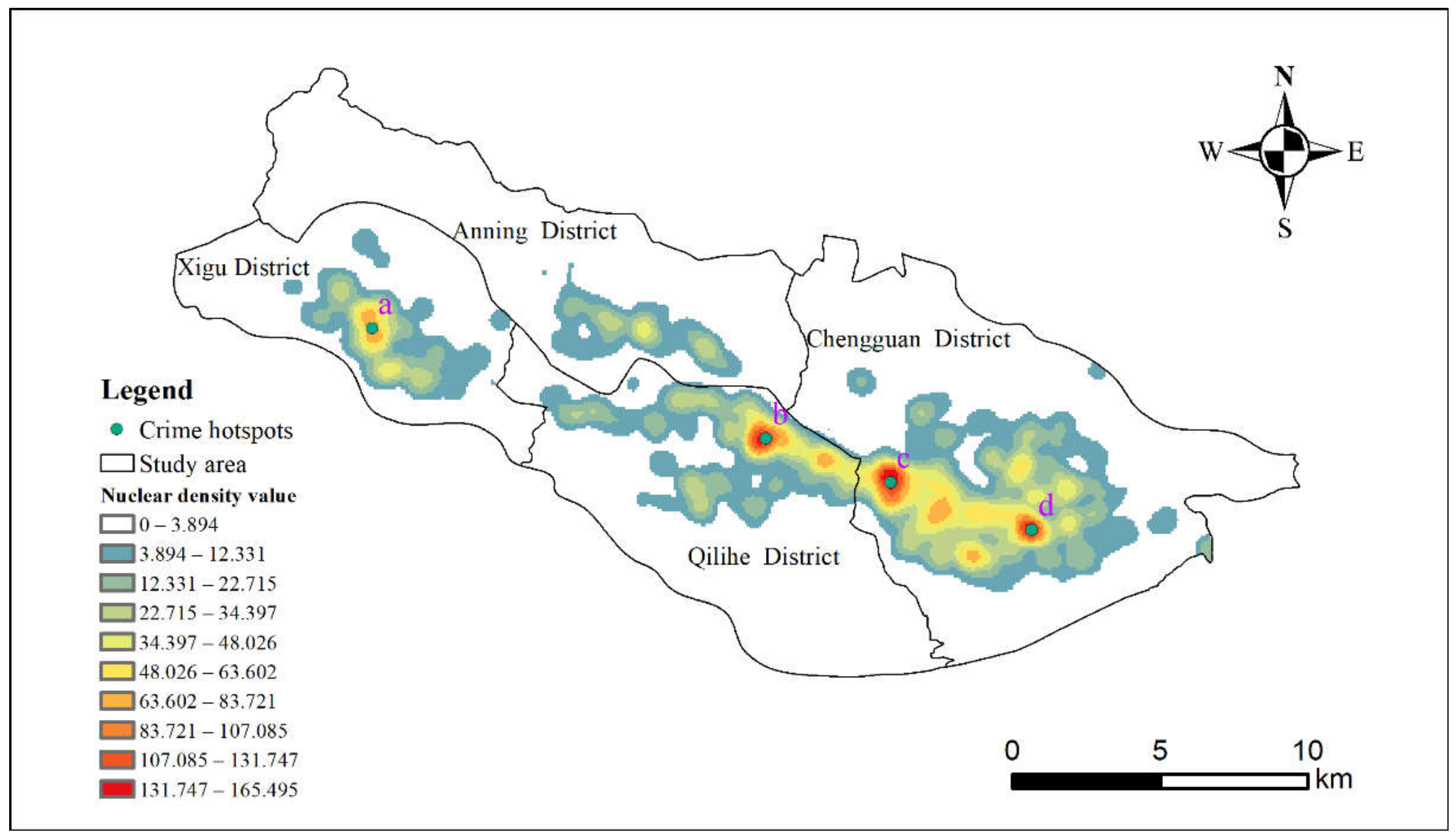
3.1. The Analysis of Spatial Distribution Heterogeneity of Property Crime

The result of the Average Nearest Neighbor showed that the A N N I index was 0.293 and the z-score was −63.511, which passed the test at the significance level of 0.01 and belonged to a significant spatial clustered pattern. Further analysis was carried out by using the KDE method, and the result was shown in Figure 4.
The distribution of property crime in the main urban area of Lanzhou had spatial heterogeneity, with the pattern of a local multi-center. Throughout the study area, crime sites were not randomly distributed, they were concentrated in some small “hot spots”. Results showed that more than half of the crime cases were concentrated in 4.33% of the area, and even up to 72.22% of crime cases were highly concentrated in 8.60% of the study area, which was consistent with previous studies [70]. In Figure 4, the crime hotspots were as follows: the crime hotspot c was near the CBD (Central Business District) in Chengguan District, where the city’s most famous sports centers, the highest-grade shopping malls, railway stations, high-grade hotels and office buildings of large domestic enterprises were located. In addition to the developed commercial, accommodation and catering industry, there were some colleges and universities, with a large number of young people, developed transportation and a high level of economic development. Crime hotspots b and d were located in the old urban areas of Qilihe District and Chengguan District, respectively, where there were dense dilapidated public housings, perfect commercial facilities, schools, tourism reception facilities, and the largest ethnic minority gathering area in the city. The crime hotspot a was located in the typical urban villages of Xigu District, where a large of floating population clustering. The exogenous of social members, cultural heterogeneity, and group vulnerability in these regions were prominent, which made government management difficult [71]. As the traditional political, cultural and educational center of Lanzhou, the south bank of the Yellow River with the well-developed economy had sound infrastructure, dense population, and was also an area with a high incidence of property crime.

3.2. Bayesian Linear Regression Analysis

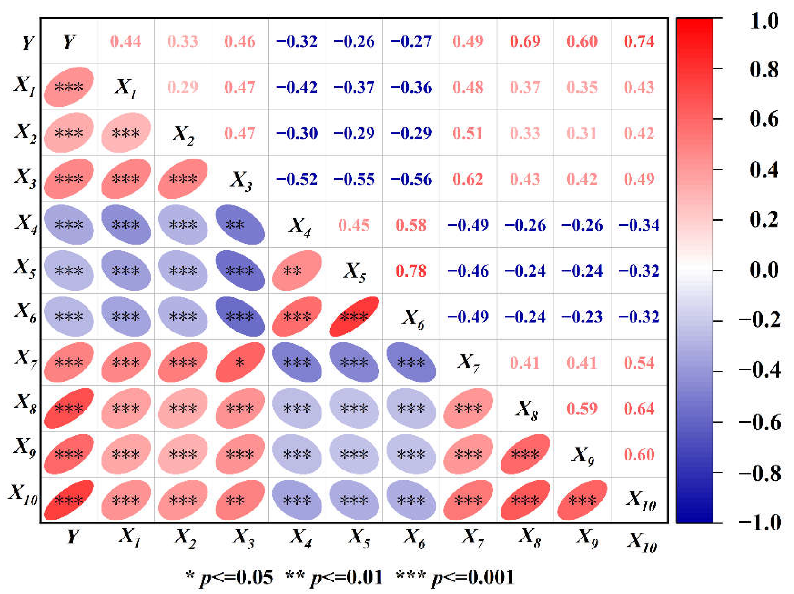
3.2.1. Multi-Collinearity Test and Pearson Analysis

The statistics of variable data are shown in Table 3. The strong correlation between variables may cause model estimation distortion, so it is necessary to carry out multi collinearity tests on independent variables. The Variance Inflation Factors (VIF) of all independent variables were less than 4.0 and the tolerance of all independent variables (1/VIF) were greater than 0.3, which was consistent with the assumption of independence of regression model characteristics [72]. Meanwhile, the Pearson correlation coefficients between each independent variable and the dependent variable Y were calculated for verifying the rationality of the independent variable selection (Figure 5). The results passed the significance test at the significance level of 0.01.
Figure 5 showed that most of the factors show a moderate or strong correlation with the crime distribution, and seven factors were positively correlated with crime distribution, among them, the max Pearson correlation coefficient value was 0.744, and shop density(X10) was the most important factor for crime distribution in the study area.

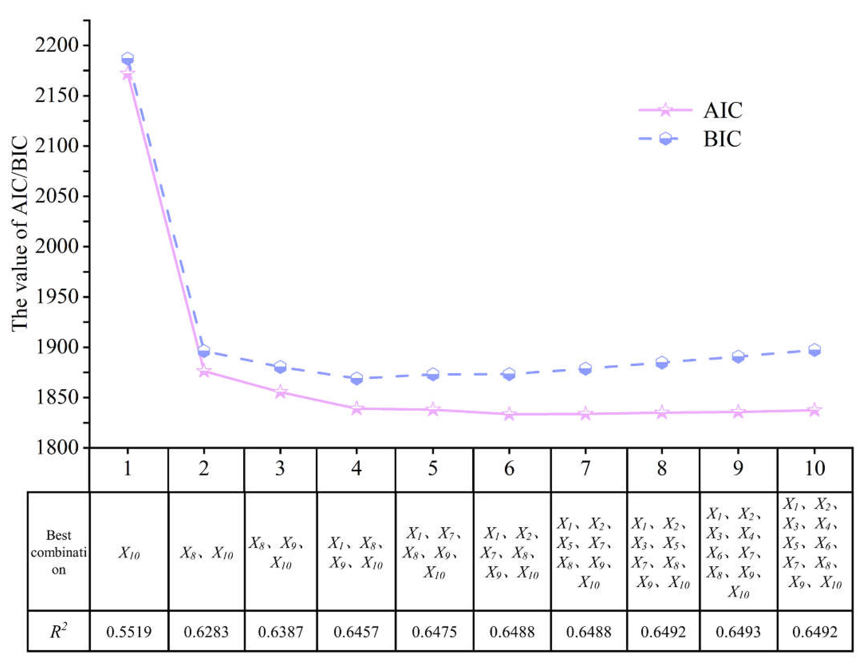
3.2.2. Regression Model with the Optimal Combination of Independent Variables

For each subset model, the combination of variables was determined by R2adj, and a total of 10 regression models were obtained, which were comprehensively evaluated the fitting to the dependent variable Y by R2. The closer the R2 is to 1, the higher the regression fitting accuracy is. Akaike Information Criterion (AIC) and Bayesian information criterion (BIC) are the criteria to measure the good fitting of statistical models based on entropy, which can effectively avoid the phenomenon of overfitting, and their smaller values indicate that the model can best explain the dependent variable with a minimum number of variables. The results of R2, AIC and BIC for the 10 regression models were shown in Figure 6. Generally speaking, with the increase of the number of model independent variables, R2 increased gradually, which occurs in the condition of the model with non-over-fitted. Figure 6 showed that the rising trend of R2 gradually slowed down and became stable when the number of independent variables n was greater than 4. When n = 4, the value of BIC reached the lowest, and then increased gradually, indicating that the model had over-fitted since then and the fitting effect of the model was the best. When n > 9, R2 did not increase accordingly. So, we have the optimal regression function based the Bayesian linear regression;
Y = 0.011 + 0.083 X 1 + 0.356 X 8 + 0.099 X 9 + 0.428 X 10 .
Equation (12) showed that the four independent variables, population density (X1), entertainment density (X8), hotel density (X9) and shop density (X10), can be used as the optimal independent variable combination to influence the distribution of property crime in the central urban area of Lanzhou. It is also found that the maximum R2 among the 10 regression models was only 0.6492 in Figure 6, indicating that crime is a complex process formed by numerous people and the microscopic role of people and the environment. Because of its inherent complexity, it is difficult to fit with high precision [73].

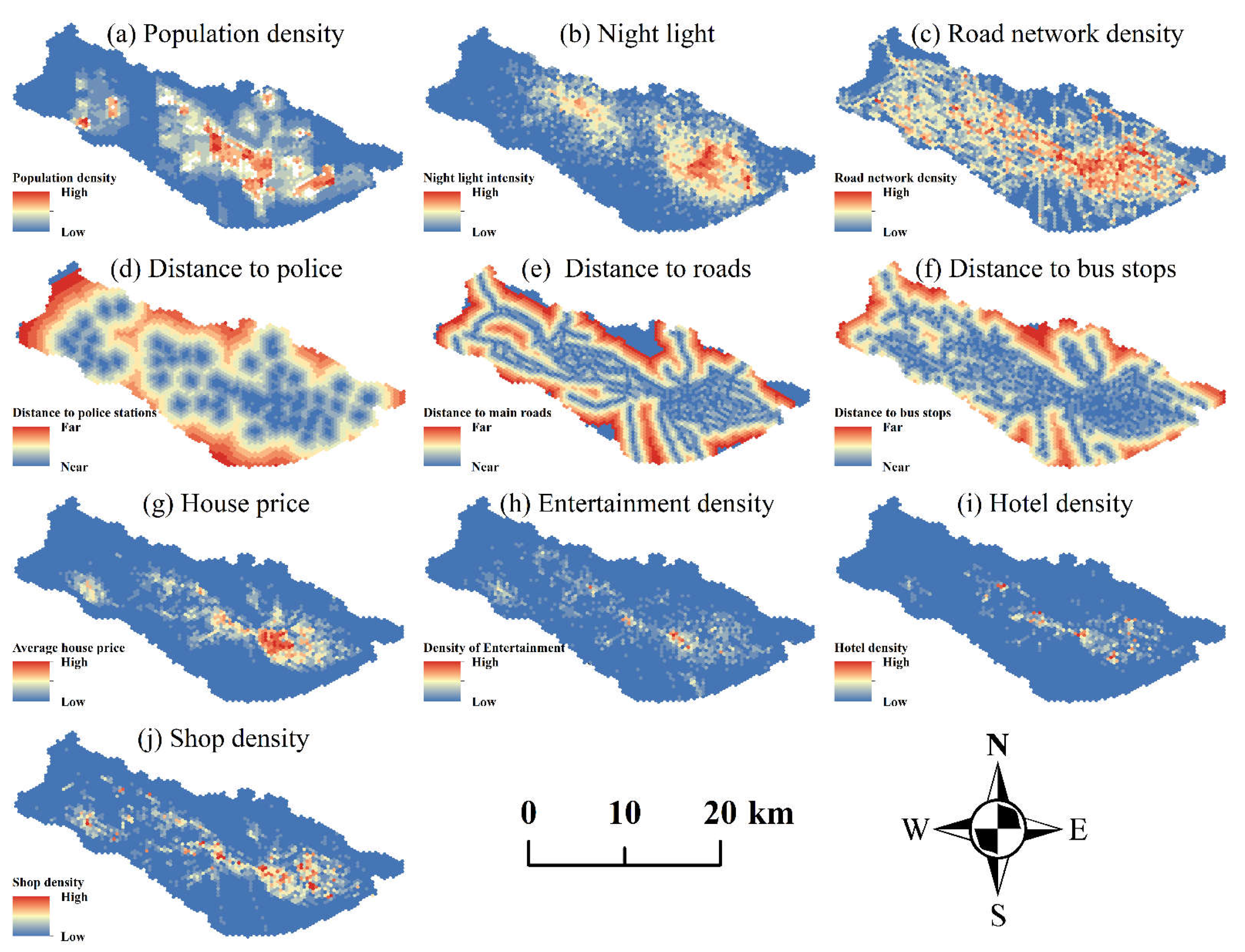
3.2.3. Analysis of Independent Factors on Crime Distribution

The Pearson correlation coefficients in Table 3 showed that house price (X7), entertainment density (X8), hotel density (X9) and shop density (X10) were positively correlated with crime distribution, which is consistent with the Equation (12). The shop density (X10) was the independent variable with the largest absolute coefficients in Equation (12), which was consistent with the strongest relationship by Pearson correlation coefficient in Table 3. The distance to the police stations (X4) was negatively correlated with crime distribution from Table 3, and the Pearson correlation coefficient was −0.324. It meant that more crime cases occurred in areas closer to the police authority.
Nighttime lighting was often used to study large spatial scale problems such as urban expansion, economic agglomeration, and human activity, while it was less applied in the field of crime geography. The launch of night light remote sensing satellite NPP and the open access to data make it possible to use night light data to study urban crime.
The samples of crime were divided into two categories according to the time of committing crime, crime committed during the day and crime committed during the night. The statistical relationship between the two categories and the night light intensity were shown in Figure 7. The R2 value fitting with the crime committed during the night was 0.191, indicating that the night light intensity in the study area had a positive impact on the crime committed during the night, but this effect was not statistically significant. The R2 value fitting with the crime committed during the day was 0.159, which was still weakly correlated. The influence of the night lighting on the property crime in Lanzhou was not significant, which might be related to the climate of Lanzhou. At 36 degrees North of the equator, Lanzhou is located in the inland of northwest China, where the annual average temperature is 10.3 °C and the winter is cold and long. The variation of temperature between the day and night is large, and the temperature at night is relatively low. Low temperature limits the outdoor socialization of residents and leads to decrease the activity intensity of residents, it plays a certain role in restricting property crime [74].
According to the routine activity theory, the conditions that lead to crime behavior include motivated offenders, appropriate targets, and the lack of crime prevention. The relationship between house price and property crime could be considered in terms of the latter two elements. On the one hand, house price represents the income level of the community to a certain extent, large gains of a successful crime from the rich attract the crime offenders, and there may be more victims in communities with higher income levels; On the other hand, the price of the house is usually proportional to the level of public security management in the community, and the higher the house price is, the more complete the security management measures may be [75].
Figure 8 showed that the property crime in the study area mainly occurred in the residential communities with the house price from 8000 to 14,000 ¥/m2, and a few criminal cases occurred in the communities with the house price less than 7500 ¥/m2 or more than 20,000 ¥/m2, and there was a peak of crime in the communities with the house price about 13,000 ¥/m2. Most of the communities with house price below 7500 ¥/m2 were located in the suburbs (Figure 8b), where the population was relatively scattered, most of the owners or tenants were migrant workers or low-income groups. There were low crime proceeds and success rate and was less attractive to criminals; The communities with house price from 8000 to 14,000 ¥/m2 were mainly located in the central urban area (Figure 8c), with high population density, convenient transportation, and most of the owners had a stable income. There was a crime peak in the communities with the house price about 13,000 ¥/m2 (Figure 8a). Most of these communities were located around the busiest urban commercial area, with high population density, dense road networks, high community openness and complex building environment, which were excellent breeding grounds for crime [76]. Communities with the house price more than 20,000 ¥/m2 were mostly located in the villa area (Figure 8d), where the security facilities were relatively complete, with strict management of the entry and exit of outsiders and perfect monitoring equipment. According to the rational choice theory, the overall income level of the owners in the villa area is higher, while the risk of crime in the villa area is often greater than the proceeds of crime. Criminals seldom choose to commit crime here through the rational trade-off between risk and proceeds, so there were fewer crime cases in the villa area [75].
The results in Table 3 and Figure 8 showed that the relation curve between property crime cases and house price showed a normal distribution curve. In the range of 0 to 13,000 ¥/m2, the property crime cases increased with the rise of the house price, after more than 13,000 ¥/m2, the crime cases decreased with the rise of the house price. The Pearson correlation coefficient showed that there was a positive correlation between house price and crime, it may be that crime cases were mainly distributed in the first half of the normal distribution curve, where the property crime cases decreased with the rise of the house price.

3.3. The Analysis of Geo-Detector Results

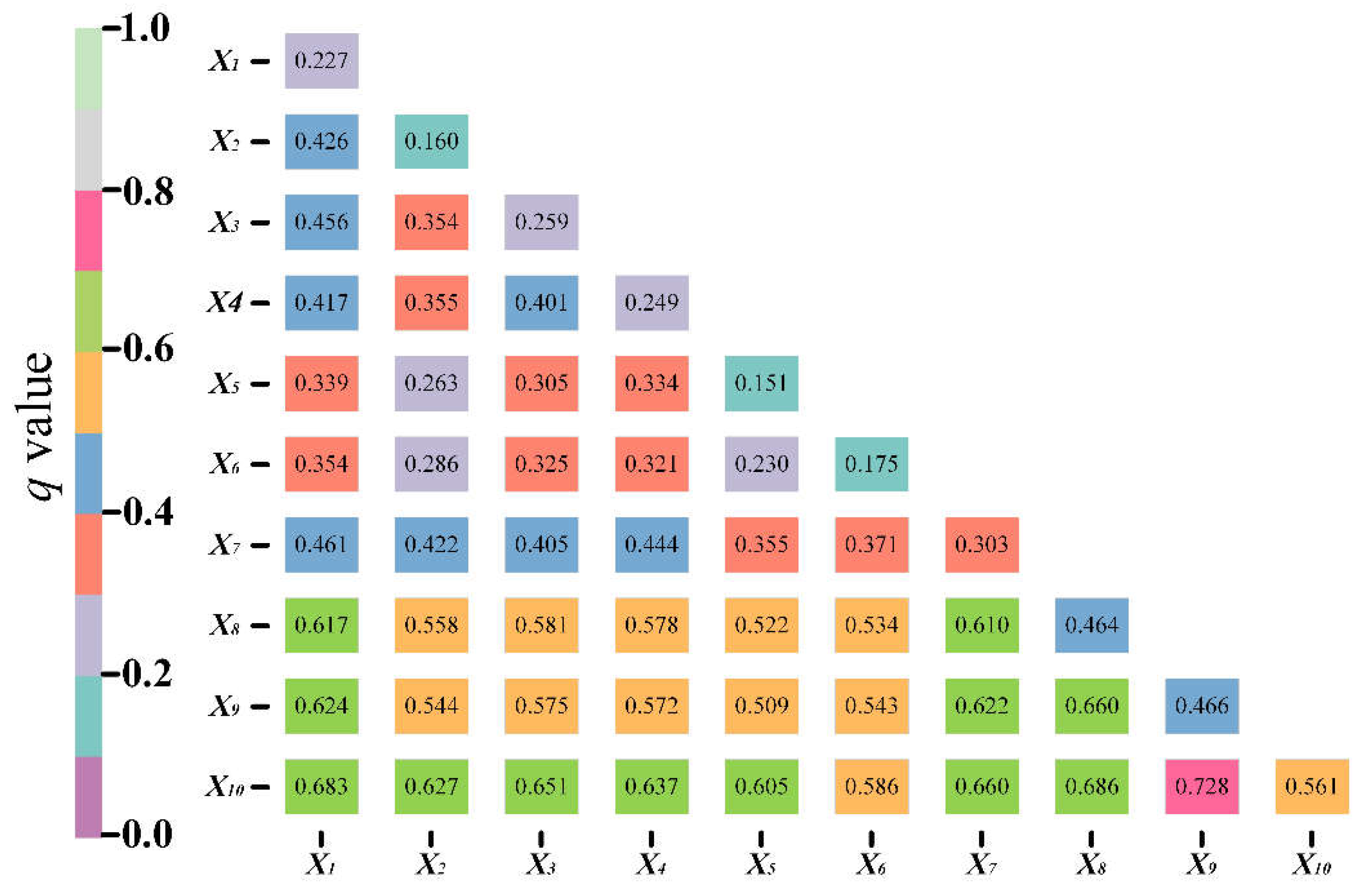
3.3.1. The Dominant Factors on Property Crime

The explanatory power of factors affecting property crime was measured with q value in Figure 9. Factors explanatory power were ranked as follows: Shop density (X10) > hotel density (X9) > entertainment density (X8) > average house price (X7) > road network density (X3) > distance to police stations (X4) > population density (X1) > night light intensity (X2) > distance to bus stops (X6) > distance to main roads (X5). Shop density (q = 0.56), hotel density (q = 0.47), entertainment density (q = 0.46) and house price (q = 0.30) were the four most powerful drivers. It showed that the commercial factors, which were related to the proceeds of crime, are the most important factors for property crime, which is consistent with previous studies [77].

3.3.2. The Differences between Factors

Ecological detection reflected whether there were significant differences in the effect of various factors on property crime. The detection results of Table 4 showed that there were no significant differences among seven couples of variables and there were significant differences among most variables. Combined with the results of the factor detector, we presented that shop density (X10), hotel density (X8) and entertainment density (X7) were the key factors for crime in the main urban area of Lanzhou, which was also consistent with the results of Bayesian linear regression. The spatial concentration of property provided attractive targets for property crime.

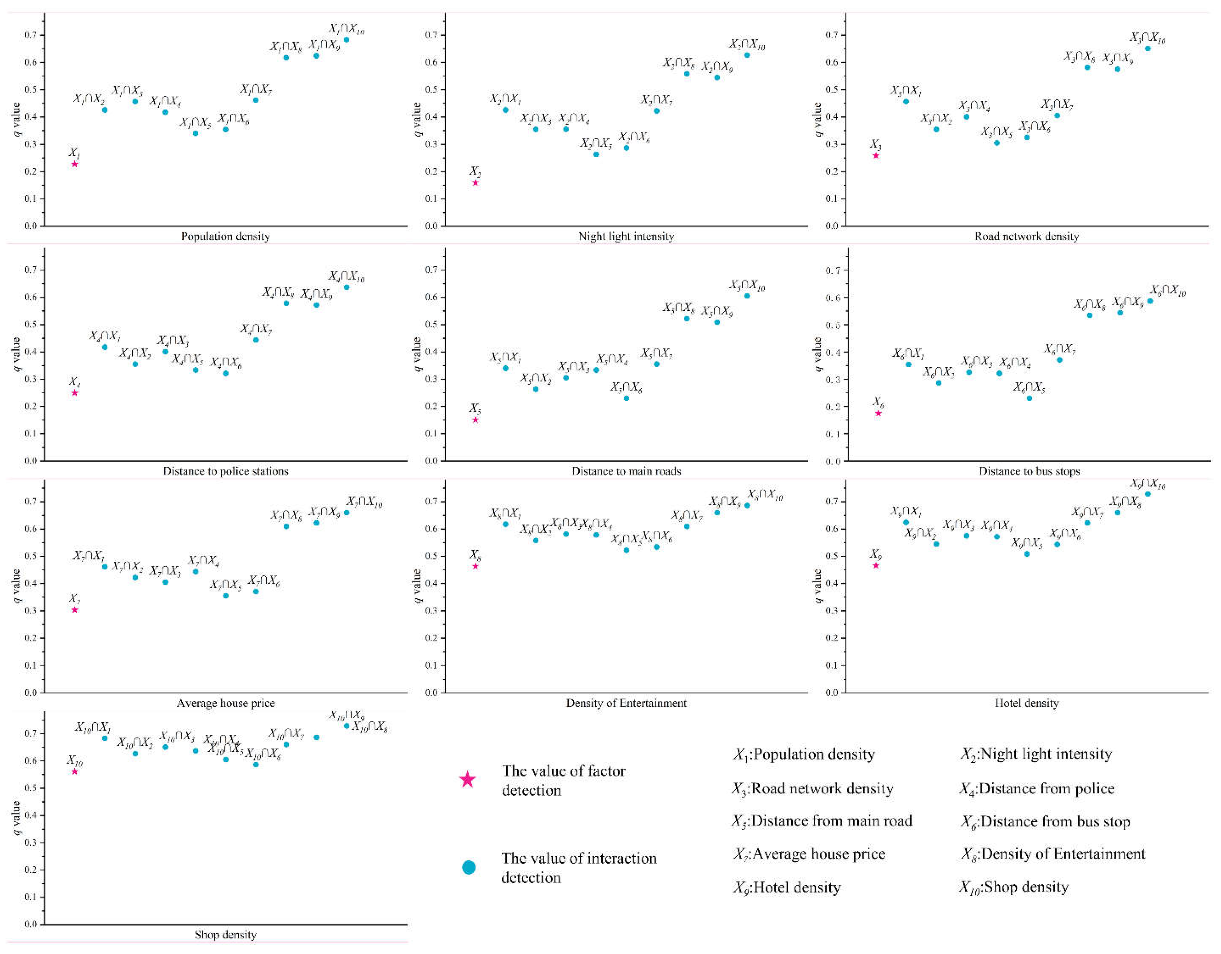
3.3.3. The Interaction of Factors on Property Crime

The interaction detector showed that the influence of any two factors was a two-factor enhancement, indicating that there was no independent factor from the system perspective. The interactions between most influencing factors showed a binary enhancement (from Table 3). Figure 10 and Figure 11 showed that the three strongest interactions were shop density ∩ hotel density (q(X10X9) = 0.728), shop density ∩ population density (q(X10X1) = 0.683) and shop density ∩ entertainment density (q(X10X8) = 0.686), and the explanatory powers between shop density and other environmental factors were also ranked in the top of all interactions. It showed that in the central urban area of Lanzhou, shop density was the most dominant factor on property crime than other factors, it had a strong interaction with environmental factors, and became an important catalyst for the occurrence of property crime.
From Figure 11, we found that without commercial factors (shop density, hotel density, entertainment density), the maximum q value of interaction was population density ∩ average house price (q(X1X7) = 0.461), which was related to the urban functional characteristics of Lanzhou. As the population center of the northwest region, the main urban area of Lanzhou has a high population density, but the urban functional space is relatively simple, basically divided into residential and commercial spaces, with few primary and secondary industries. The sub-high q value of interaction was the population density ∩ road network density (q(X1X3) = 0.456) without commercial factors. It showed that in the areas with high flow of people and convenient transportation, the chance of committing crime was much higher. The dense and developed road network facilitated the escape after committing the crime. It was necessary to emphasize that in the interaction detections, the influence of population density alone and road network density alone on crime was not significant. It meant that only high population density or convenient transportation would not greatly increase the probability of crime, but when the two work together, the probability of crime would be greatly increased. This was also consistent with the routine activity theory that crime requires a potential victim and a suitable environment to occur [17].
In addition to the binary enhancement, there was also a non-linear enhancement (from Table 3) between population density and night light intensity (q(X1X2) = 0.426 > q(X1) + q(X2)). The higher the population density and night light intensity, the higher the explanatory power on property crime, which was greater than the sum of the two factors alone. This indicated that there was a strong complementary relationship between night light intensity and population density among the factors affecting crime, and the night light provides a better view and convenience for criminals to commit crime in the crowd.

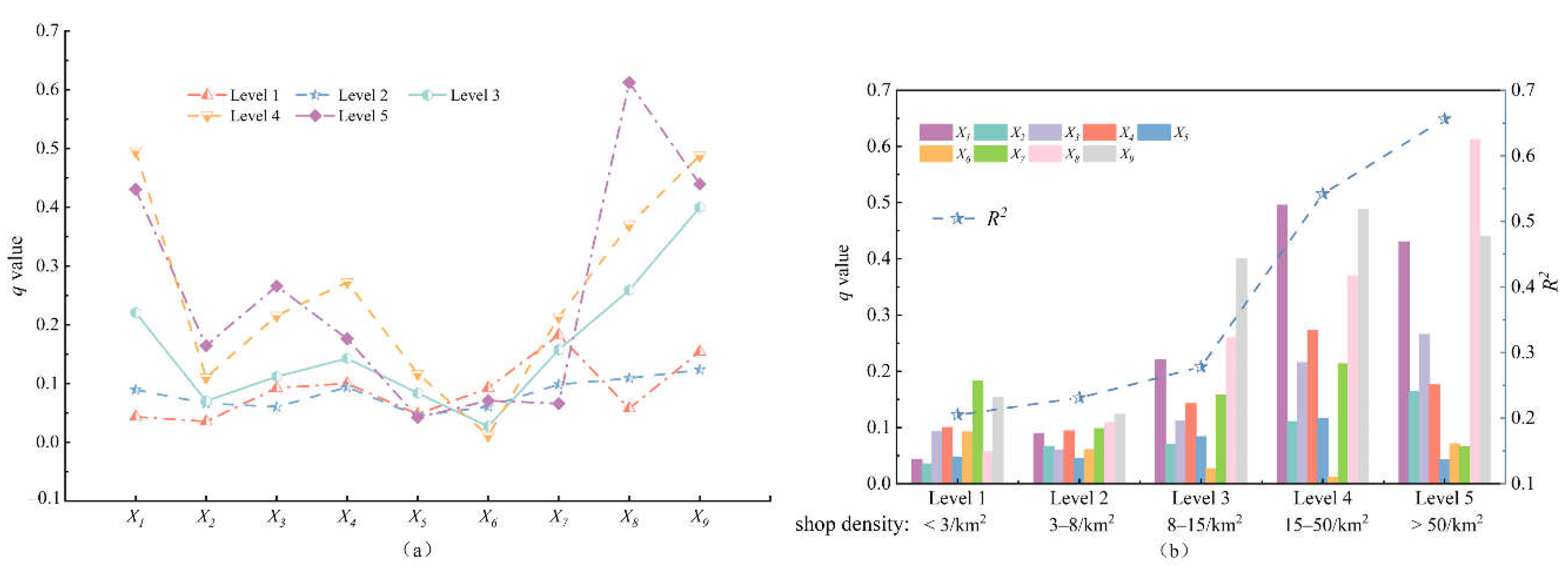
3.3.4. Influence of Factors on the Stability of System Interpretation

Both Bayesian linear regression and geo-detection showed that shop density was the most important factor affecting property crime in the main urban area of Lanzhou. According to the natural breakpoint method, the shop density was divided into five grades:0–3 (level 1), 3–8 (level 2), 8–15 (level 3), 15–50 (level 4), >50 (level 5), and the changes of the other environmental factors on property crime with different shop density gradient were discussed.
Figure 12a showed that in the urban area with level1, the average house price (X7) was the main factor affecting crime. With the increase of the shop density, population density (X1), entertainment density (X8) and hotel density (X9) became the main factors for crime, and the q values kept getting larger. It might be that with the prosperity of commerce, the surrounding hotels and entertainments were also increasing, these facilities attracted more people, and these leisure and entertainment places themselves were areas with a high incidence of crime. When the shop density was highest (level 5), population density (X1), entertainment density (X8) and hotel density (X9) were still the main factors affecting crime, while the q value of house prices was weak. The area with level 5 was located in the central business district, far from residential areas.
It could be seen from Figure 12a that with the continuous increase of shop density, the q value curves fluctuated significantly, and the solution of the model tended to be unstable. It indicated that with the continuous increase of shop density and the gradual transition from residential areas to commercial areas, the environmental factors gradually became complex. This led to the instability of the crime interpretation system and the sharp fluctuations of explanatory power curves. For better understanding the environmental mechanism behind property crime, we established regression equations between factors and property crime under different levels of shop density, and the R2 was shown in Figure 12b. The R2 showed that with the increase of the shop density, the fitting accuracy of various factors to property crime was improved.

4. Discussion

This paper explored the factors driving property crime by combining factor regression and factor interaction in Lanzhou city, China. We measured the spatial clustered pattern of crime by ANN index and KDE, presented Bayesian methodology for factors estimation on spatial heterogeneity of crime and used the best subset selection model to fit the effect on the dependent variable by containing the least number of free variables. The Bayesian linear regression could simulate the characteristics of the dependent variable with independent variables, but it does not consider the interactions between variables, which is insufficient for a systematic understanding of the geographic phenomena. Compared with the regression model, Geo-detector investigates the interaction between two explanatory variables to the response variable in the process of measuring and finding spatial stratified heterogeneity, which is an effective method to study driving factors, but it lacks the ability of regression models to simulate the characteristics of the dependent variable. In this paper, we explored the factors influencing crime cases distribution in Lanzhou by coordinating factor regression and factor interaction.
Generally speaking, crime is a rare event. The distribution of crime cases in the main urban area of Lanzhou had the spatial heterogeneity, with the pattern of local multi-center, which reflected the nonrandom spatial distribution. The results showed that more than half of the crime cases were concentrated in 4.33% of the area, and even up to 72.22% of crime cases were highly concentrated in 8.60% of the study area. The risk of suffering crime was not uniformly distributed over a region, and there were places in which crime cases were concentrated, which was consistent with previous studies [70,78]. These property crime hotspots are mainly concentrated in the CBD, universities, as well as slums. CBD is an area with wealth. Colleges and universities are concentrated areas of students as well as high valuable electronic products, such as mobile phones, laptops, iPad, etc. According to the routine activities theory (RAT) [17], criminals will choose valuable things that are is small and easy to hide in the same conditions, that is, criminals will prefer mobile phones to computers that are not easy to carry. The buildings in slums are dilapidated, the floating population is large, and the crime prevention is weak. The attractive targets which are from the concentration of wealth, and the lack of capable guardianship contribute to the offenders’ access to suitable, insufficiently guarded targets, whose spatial heterogeneity formed the spatial distribution of property crime. As such, offenders have been described as foragers, who “must find a good hunting ground before starting to chase prey” [79], then CBD, colleges, universities and slums are good hunting ground in offenders’ sight, which is in line with the crime pattern theory.
Every crime is an intersection of two factors in time and space: an offender’s motivation to commit a crime and the opportunity to carry out the desired act in a particular situation [80]. The results of the independent factors indicated that the explanatory power (q value) of different factors on the spatial distribution of crime were shop density (X10) > hotel density (X9) > entertainment density (X8) > average house price (X7) > road network density (X3) > distance to police stations (X4) > population density (X1) > night light intensity (X2) > distance to bus stops (X6) > distance to main roads (X5). Shop density (q = 0.56), hotel density (q = 0.47), entertainment density (q = 0.46) and house price (q = 0.30) were the four most powerful drivers, and those 4 factors were also the independent variables with the largest absolute Pearson coefficients. As factors reflecting attractive targets, Shop density, hotel density, entertainment density and house price are important factors on property criminals’ motivation in rational choice theory. The Pearson coefficient values of those 4 factors were all larger than 0. This meant that these four factors might induce the occurrence of property crime, or the regions with high values of these four factors were more attractive to property crime, which seems to be more appreciated by traditional criminal scholars. It was also found that the maximum R2 among the regression functions was only 0.6492, that is, crime is a complex process formed by numerous people and the microscopic role of people and the environment. For its inherent complexity, it is difficult to simulate or predict the crime location with high precision.
The Pearson coefficient values of distance to police stations (X4), distance to main roads (X5), and distance to bus stops (X6) were all less than 0, they had a weakly negative impact on crime. Although it is generally believed that the police station is a deterrent point to crime [41], representing a parameter for the expected value of getting caught [80] and does not seem to be attractive to offenders. If the rational choice or routine activity theory is adopted, a potential offender will choose the furthest point from a police station to commit a crime [81], while a number of studies have shown that proximity to a police station appears to increase property crime [71,82]. Possible reasons for this finding were as follows: It was police station patrol, not a station building, that had a more effective deterrent effect on crime, and there was no evidence that patrol around police station buildings was more intense than in other areas. In addition to crime prevention, the daily work of police includes interacting with the neighborhood population (Household management, in China), listening to their needs and proposals, and providing reliable information for decision making, so it is generally closer to the community, residents and commercial facilities, that is, it is closer to the hot spot of crime. Victims of theft might be more likely to notify the police if victimization takes place near a police station [71]. We cannot entirely exclude the possibility that our results are in part driven by differences in police manpower and changed patrolling intensity. This is because we lack more detailed data on police patrol records to assess the impact of the patrol intensity around police stations on the incidence of crime, which is related to the perceived risk of respective criminal offenders.
It has long been thought that street lighting can affect crime, and three research projects carried out in Dudley, Stoke-on-Trent and New York found that increased levels of lighting led to crime reduction [26,83]. The results in this paper showed that the light intensity in the study area had a positive effect on crime committed. The two conclusions seem to be contradictory. In fact, for the same area (such as a community), the light intensity in different periods is negatively related to crime, that is to say, improving lighting reduces the crime in this area, while for the crime space heterogeneity of cities in the same period, lighting is positively affecting crimes committed, that is to say, the higher the light intensity, the more crimes committed. The relationship between light intensity and property crime has different correlation explanations in temporal projection and spatial projection. The intensity of night light essentially reflects human activity. Factors that inhibit human activity, such as severe cold, will reduce the correlation coefficient between the night light intensity and the crime space heterogeneity of cities, therefore we can make a prediction that the correlation coefficient between the night light intensity and the crime space heterogeneity of cities in the cold zone might be lower than that in the temperate zone or the tropics.
This paper analyzed the correlation between the house price and property crime. Taking into account the exchange rate difference of the currencies of various countries, Price-to-Earnings Ratio (PE Ratio) was introduced into the analysis, which was calculated as follows:
PE Ratio = Average City house price/Cities average full time mean monthly earnings,
where the value of City average full time mean monthly earnings for Lanzhou city was 2471¥/month [84], and the unit of Average City house price was ¥/m2.
The statistical results showed that there was a normal distribution curve between the number of property crimes and the PE Ratio of the community. Combined with the definition of PE Ratio and calculated from the data in Figure 8, the crime in the study area mainly occurred in the residential communities with the PE Ratio from 3.0 to 6.0, and a few criminal cases occurred in the communities with the PE Ratio less than 3.0 or higher than 8.0, the crime peak occurred in the communities where the PE Ratio was about 5.26. The regions with low PE value were mostly apart from the city center, where low-and-middle income groups gathered, and the expected gains of committing a crime were small, which caused property crime to decrease. Wealthier urban dwellers mostly gathered the regions with high PE value. Although wealthier individuals were more economically attractive to criminals, the self-segregation of the wealthier urban dwellers increased to protect their property and individual privacy. They lived in gated communities. Gated communities in most cities were generally planned as a whole and designed with sophisticated security measures, such as electronic doorman systems, provided by the project developers, which effectively deterred the potential offenders and reduced property crime. For property offenders, they were less likely to choose areas with stronger guardianship.
Most scholars in traditional criminology and environmental criminology studied factors on criminal behavior as independent individuals, without a care about factor interaction. The results of the factor interaction indicated that shop density had the strongest interaction with other factors, and the interactions of shop density ∩ hotel density (q(X10X9) = 0.728), shop density ∩ population density (q(X10X1) = 0.683) and shop density ∩ entertainment density (q(X10X8) = 0.686) were the three strongest interactions, reflecting that shop density not only had a great influence on property crime, but also had a strong interaction with environmental factors, and has become an important catalyst for the occurrence of property crime. It also found that both factor interactions showed a two-factor enhancement, and the explanatory power of the factor interactions for property crime was much greater than any single factor, which was in line with Place Management Theory. The q values of factor interaction were less than the sum of q value of single factor, indicating that the interpretation of environmental factors to crime was not completely statistically independent, that is, multiple environmental factors might not work in an independent manner. It revealed that property crime was highly likely when multiple positive environmental factors come together at the same place at the same time. For example, in CBD, a busy street with near access to a bus-stop or high-way offers more lax place-level opportunity for property crime. From the perspective of crime complexity, the spatial heterogeneity of property crime is the result of the comprehensive interaction of multiple factors [85], and the feedbacks between economic and environmental factors influencing property crime spatial heterogeneity are complex. The results of factor interaction well illustrated this point, which also reminded us to study the deep driving forces of property crime from a systemic perspective. The value of a positive correlation between shop density and property crime was the largest among the socioeconomic drivers, which reflected that gain was the primary goal of property crime. This paper also discovered that the shop density gradient influenced the degree of interpretation of spatial heterogeneity of property crime in the main urban area of Lanzhou. With the continuous increase of shop density, the q value curves fluctuated significantly, the solution of the model tended to be unstable, and the fitting accuracy of various factors affecting crime was improved.

5. Conclusions

This paper focuses on the physical and social environmental factors affecting property crime, which belongs to the category of environmental criminology. A combination of factor regression and factor interaction was proposed to explore the drivers on the spatial heterogeneity of property crime, based on property crime records data and some socioeconomic data, including house price, population density, shop density, bus stops, entertainment, hotels, police stations, and other environmental data, such as road and night lighting. We took the main urban area of Lanzhou, China, as a case to analyze the results. The main conclusions were as follows.
(1)
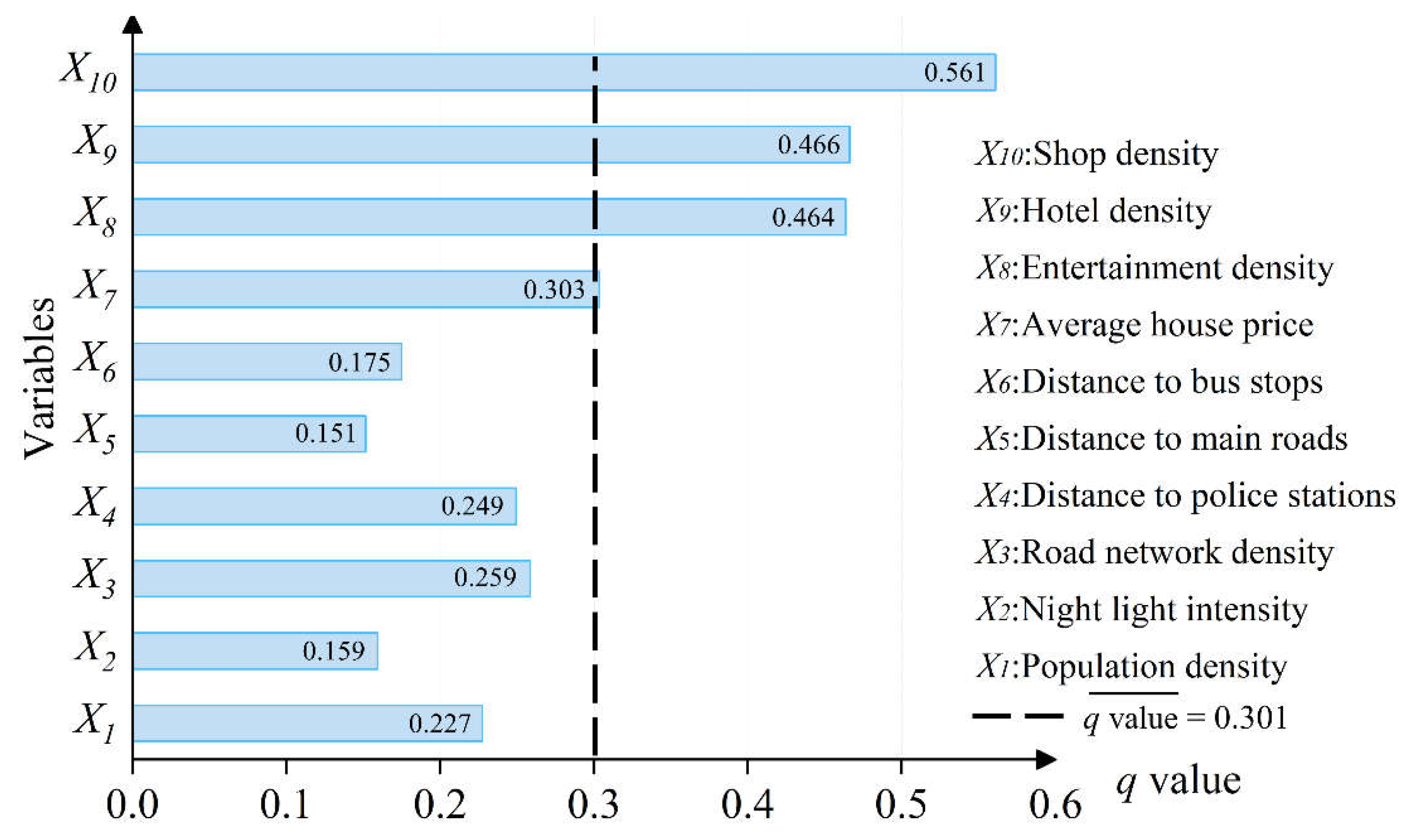
The distribution pattern of property crime cases in the main urban area of Lanzhou was not non-random; it had spatial heterogeneity, more specifically, spatial agglomeration. Half of the crime cases were concentrated in 4.33% of the area, and even up to 72.22% of crime cases were highly concentrated in 8.60% of the study area. Shop density, hotel density, entertainment density and house price were the four most powerful drivers of the spatial distribution of property crimes in the main urban area of Lanzhou, and the regions with high values of these four factors seemed more attractive to property crime. The attractive targets, which are from the concentration of wealth and the lack of capable guardianship, contribute to the offenders’ access to suitable, insufficiently guarded targets, whose spatial heterogeneity leads to the spatial distribution of property crime;
(2)
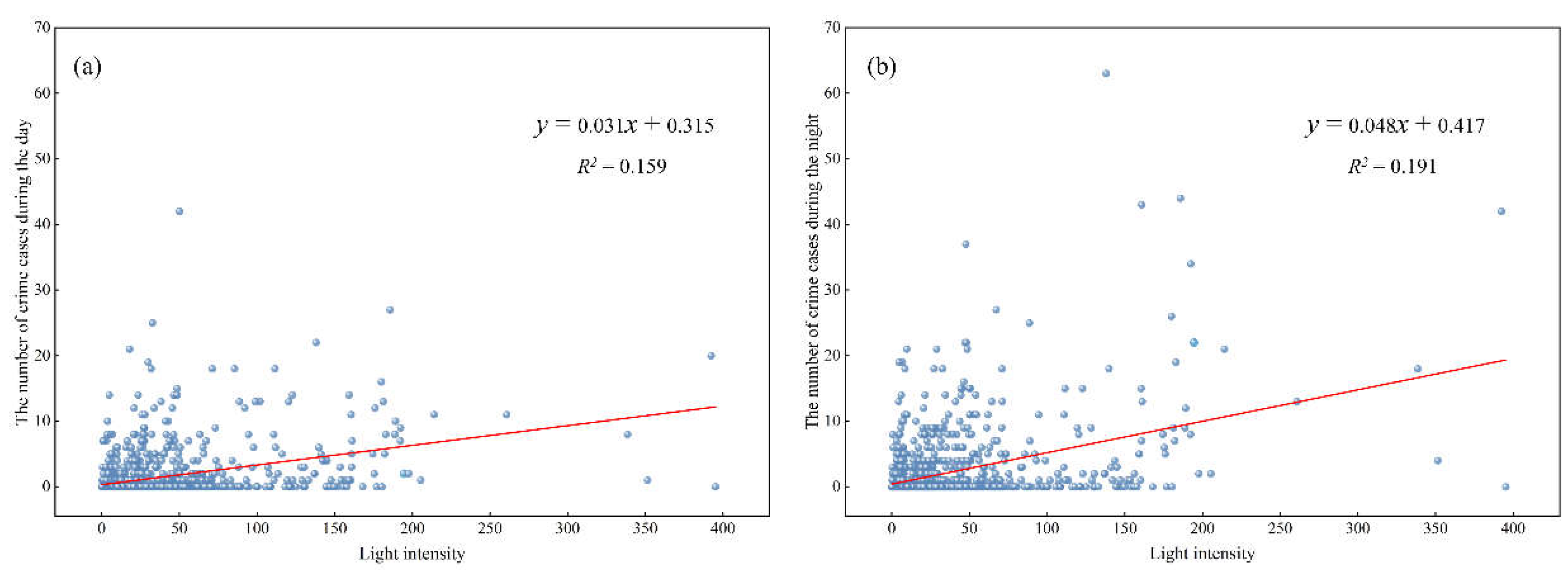
The distance to police stations, distance to main roads, and distance to bus stops had a weakly negative effect on property crime. The light intensity in the study area had a positive effect on crime committed. The relationship between the light intensity and crime has different correlation explanations in temporal projection and spatial projection. Factors that inhibit human activity, such as severe cold, will reduce the correlation coefficient between the night light intensity and the crime. We can make a prediction that the correlation coefficient between the night light intensity and the crime of cities in the cold zone should be lower than that in the temperate zone or the tropics;
(3)
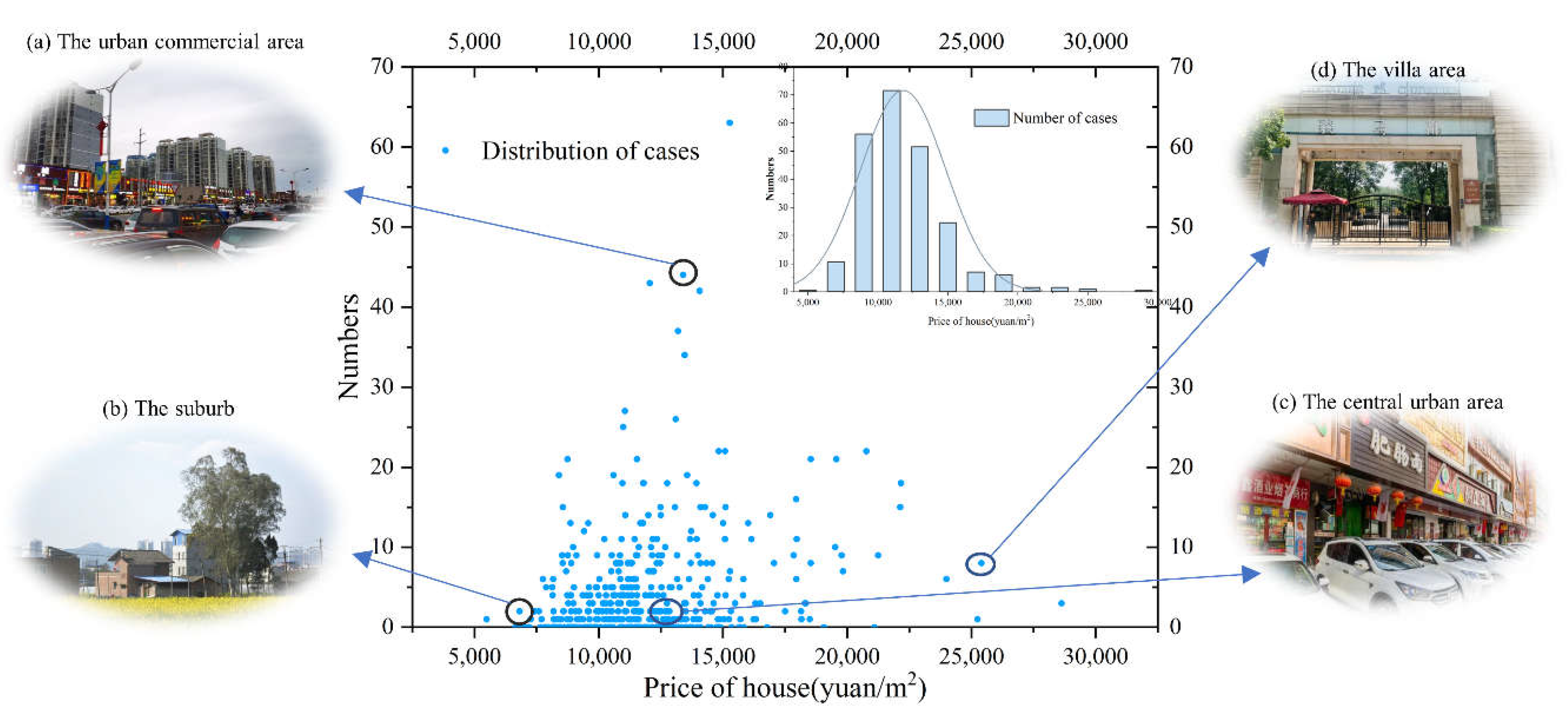
There was a normal distribution curve between the number of property crimes and the PE ratio of the community. With the increase of PE ratio, the number of property crimes first increased and then decreased, and the peak PE ratio was 5.25. Gated communities were designed with stronger guardianship, which effectively deterred the potential offenders and reduced property crime. For property offenders, they were less likely to choose areas with stronger guardianship;
(4)
The results of the factor interaction indicated that multiple environmental factors might not work in an independent manner; factor interactions showed a two-factor enhancement, and the explanatory power of the factor interaction for property crime was much greater than any single factor. As an important catalyst, shop density had the strongest interaction with other factors. The shop density gradient influenced the degree of interpretation of spatial heterogeneity of property crime. With the continuous increase of shop density, the solution of model factors tended to be unstable, and the fitting accuracy of various factors to crime was improved. Even so, the maximum R2 among the regression functions was only 0.6492, that is, the crime action is a process formed by multiple microscopic roles of people and the environment. For its inherent complexity, it is difficult to simulate or predict the crime event location with high precision.
This paper studied the environmental criminogenic contexts and exemplified environmental inducement for criminal action. However, limitations are evident. The statistical results in this study come from geographic information databases and urban property crime records. A criminogenic context is, itself, not sufficient for choosing crime. Socioeconomic and law enforcement variables, such as transience of the population, racial and ethnic makeup, composition by age and gender, educational levels, family structures, as well as strength (personnel and other resources) and the aggressiveness of a jurisdiction’s law enforcement agencies, should be taken into account, and through a combination of criminal investigation to further identify the causes of the results. The analysis of the inhabitant’s perception of insecurity could also be integrated into the analysis and compared with other geographical areas trying to understand possible similarities, recurrences or differences, providing a cross-reading interpretation of the results. In particular, it is necessary to clarify the coupling mechanism of criminology theory reflected by factor interaction. In addition, the analysis of the crime rate instead of crime density as a dependent variable is also worth exploring. Finally, the model used can be further improved. The Poisson regression is widely used for describing the frequency of random events, which is in line with the characteristics of crime occurrence. In future work, we will consider introducing Poisson regression to analyze crime cases and compare with existing results to better understand the mechanisms and factors influencing crime occurrence.

Author Contributions

Conceptualization, Lijian Sun and Guozhuang Zhang; Formal analysis, Guozhuang Zhang and Li Sun; Investigation, Guozhuang Zhang and Dan Zhao; Methodology, Lijian Sun, Guozhuang Zhang and Dan Zhao; Validation, Ling Ji and Haiyan Gu; Writing—original draft, Lijian Sun and Guozhuang Zhang; Writing—review & editing, Lijian Sun, Guozhuang Zhang, Dan Zhao and Xia Li. All authors have read and agreed to the published version of the manuscript.

Funding

This study was supported by the Fundamental Research Funds for Central Public-Interest Scientific Institution, China (No. AR2123), and in part by the Beijing Natural Science Foundation (No. 9212001).

Institutional Review Board Statement

Not applicable.

Informed Consent Statement

Not applicable.

Data Availability Statement

Some data used during the study are confidential and may only be provided with restrictions.

Acknowledgments

We appreciate Leyi Zhang from the School of Earth Science and Resources at Chang’an University for his help.

Conflicts of Interest

The authors declare no conflict of interest.

References

  1. Un-Habitat. Enhancing Urban Safety and Security: Global Report on Human Settlements 2007; Routledge: Abingdon-on-Thames, UK, 2012. [Google Scholar]
  2. Jin, G.; Shou, J.; Lin, X.N. Analysis and forecast of China’s crime situation (2018–2019). J. People Public Secur. Univ. China 2019, 35, 1–11. [Google Scholar]
  3. Matlovičová, K. Theoretical Framework of the Intra-Urban Criminality Research: Main Approaches in the Criminological Thought. Folia Geogr. 2014, 56, 29–40. [Google Scholar]
  4. Li, C.K. The applicability of social structure and social learning theory to explain intimate partner violence perpetration across national contexts. J. Interpers. Violence 2022, 08862605211072166. [Google Scholar] [CrossRef] [PubMed]
  5. Shaw, C.R.; Moore, M.E. A Delinquency Area; University of Chicago Press: Chicago, IL, USA, 1931. [Google Scholar]
  6. Harris, H.M.; Nakamura, K.; Bucklen, K.B. Do cellmates matter? A causal test of the schools of crime hypothesis with implications for differential association and deterrence theories. Criminology 2017, 56, 87–122. [Google Scholar] [CrossRef]
  7. Ward, J.T.; McConaghy, M.; Bennett, J. Differential Applicability of Criminological Theories to Individuals? The Case of Social Learning vis-à-vis Social Control. Crime Delinq. 2017, 64, 510–541. [Google Scholar] [CrossRef]
  8. Roach, J.L. Fleisher: The Economics of Delinquency (Book Review). Soc. Forces 1967, 45, 462. [Google Scholar]
  9. Becker, G.S. Crime and punishment: An economic approach. In The Economic Dimensions of Crime; Palgrave Macmillan: London, UK, 1968; pp. 13–68. [Google Scholar] [CrossRef] [Green Version]
  10. Piroozfar, P.; Farr, E.R.; Aboagye-Nimo, E.; Osei-Berchie, J. Crime prevention in urban spaces through environmental design: A critical UK perspective. Cities 2019, 95, 102411. [Google Scholar] [CrossRef]
  11. Hodgkinson, T.; Farrell, G. Situational crime prevention and Public Safety Canada’s crime-prevention programme. Secur. J. 2018, 31, 325–342. [Google Scholar] [CrossRef] [Green Version]
  12. Matlovičová, K.; Mocák, P.; Andrejko, J. Objektívna a Subjektívna Dimenzia Stavu Kriminality na Území Mesta Prešov/Prešov City Crime Perception-Draw a Comparison Situation in 2007 and 2011. Folia Geogr. 2012, 54, 146. [Google Scholar]
  13. Matlovicová, K.; Mocák, P.; Kolesárová, J.; Kvetoslava, M.; Peter, M.; Jana, K. Environment of estates and crime prevention through urban environment formation and modification. Geogr. Pannonica 2016, 20, 168–180. [Google Scholar] [CrossRef]
  14. Chainey, S.; Ratcliffe, J. GIS and Crime Mapping; John Wiley & Sons: Hoboken, NJ, USA, 2013. [Google Scholar]
  15. Rey, S.J.; Mack, E.A.; Koschinsky, J. Exploratory space-time analysis of burglary patterns. J. Quant. Criminol. 2012, 28, 509–531. [Google Scholar] [CrossRef]
  16. Leitner, M. Crime Modeling and Mapping Using Geospatial Technologies; Springer Science & Business Media: Berlin/Heidelberg, Germany, 2013; Volume 8. [Google Scholar]
  17. Cohen, L.E.; Felson, M. Social change and crime rate trends: A routine activity approach. In Classics in Environmental Criminology; Routledge: Abingdon-on-Thames, UK, 1979; pp. 588–608. [Google Scholar]
  18. Clarke, R.V.; Cornish, D.B. Modeling Offenders’ Decisions: A Framework for Research and Policy. Crime Justice 1985, 6, 147–185. [Google Scholar] [CrossRef]
  19. Brantingham, P.J.; Brantingham, P.L. Environmental criminology: From theory to urban planning practice. Stud. Crime Crime Prev. 1998, 7, 31–60. [Google Scholar]
  20. Andresen, M.A. Crime measures and the spatial analysis of criminal activity. Br. J. Criminol. 2006, 46, 258–285. [Google Scholar] [CrossRef]
  21. Short, M.B.; Brantingham, P.J.; Bertozzi, A.L.; Tita, G.E. Dissipation and displacement of hotspots in reaction-diffusion models of crime. Proc. Natl. Acad. Sci. USA 2010, 107, 3961–3965. [Google Scholar] [CrossRef] [Green Version]
  22. Ceccato, V.; Moreira, G. Research. the dynamics of thefts and robberies in São Paulo’s Metro, Brazil. Eur. J. Crim. Policy Res. 2021, 27, 353–373. [Google Scholar] [CrossRef]
  23. Liu, L.; Lan, M.; Eck, J.E.; Kang, E.L. Assessing the effects of bus stop relocation on street robbery. Comput. Environ. Urban Syst. 2020, 80, 101455. [Google Scholar] [CrossRef]
  24. Hipp, J.R.; Lee, S.; Ki, D.; Kim, J.H. Measuring the Built Environment with Google Street View and Machine Learning: Consequences for Crime on Street Segments. J. Quant. Criminol. 2021. [Google Scholar] [CrossRef]
  25. Boivin, R. Routine activity, population (s) and crime: Spatial heterogeneity and conflicting Propositions about the neighborhood crime-population link. Appl. Geogr. 2018, 95, 79–87. [Google Scholar] [CrossRef]
  26. Chalfin, A.; Hansen, B.; Lerner, J.; Parker, L. Reducing Crime Through Environmental Design: Evidence from a Randomized Experiment of Street Lighting in New York City. J. Quant. Criminol. 2022, 38, 127–157. [Google Scholar] [CrossRef]
  27. Fotios, S.A.; Robbins, C.J.; Farrall, S. The effect of lighting on crime counts. Energies 2021, 14, 4099. [Google Scholar] [CrossRef]
  28. Jacobs, R. Reclaiming the Streets of Three Rivers: Eblockwatch and CPTED. In Proceedings of the 9th Annual International CPTED Conference, Brisbane, Australia, 13–16 September 2004. [Google Scholar]
  29. Osgood, D.W. Poisson-Based Regression Analysis of Aggregate Crime Rates. J. Quant. Criminol. 2000, 16, 21–43. [Google Scholar] [CrossRef]
  30. Cabrera-Barona, P.F.; Jimenez, G.; Melo, P. Types of Crime, Poverty, Population Density and Presence of Police in the Metropolitan District of Quito. ISPRS Int. J. Geo-Inf. 2019, 8, 558. [Google Scholar] [CrossRef] [Green Version]
  31. Kondo, M.; Hohl, B.; Han, S.; Branas, C. Effects of greening and community reuse of vacant lots on crime. Urban Stud. 2015, 53, 3279–3295. [Google Scholar] [CrossRef] [Green Version]
  32. Cundiff, K. Colleges and Community Crime: An Analysis of Campus Proximity and Neighborhood Crime Rates. Crime Delinq. 2021, 67, 431–448. [Google Scholar] [CrossRef]
  33. China Judgements Online. Available online: https://wenshu.court.gov.cn/ (accessed on 1 May 2022).
  34. Zheng, Z.Q.; Jiang, C.; Yu, R.L.; Zhou, J.Q.; Wu, Z.J.; Luo, J.Y. General characteristics, economic burden, causative drugs and medical errors associated with medical damage litigation involving severe cutaneous adverse drug reactions in China. J. Clin. Pharm. Ther. 2020, 45, 1087–1097. [Google Scholar] [CrossRef]
  35. Cai, R.L.; Tang, J.; Deng, C.H.; Lv, G.F.; Xu, X.H.; Sylvia, S.; Pan, J. Violence against health care workers in China, 2013–2016: Evidence from the national judgment documents. Hum. Resour. Health 2019, 17, 103. [Google Scholar] [CrossRef]
  36. Shao, M.L.; Newman, C.; Buesching, C.D.; Macdonald, D.W.; Zhou, Z.M. Understanding wildlife crime in China: Socio-demographic profiling and motivation of offenders. PLoS ONE 2021, 16, e024608. [Google Scholar] [CrossRef]
  37. Bagan, H.; Yamagata, Y. Analysis of urban growth and estimating population density using satellite images of nighttime lights and land-use and population data. GISci. Remote Sens. 2015, 52, 765–780. [Google Scholar] [CrossRef]
  38. Pandey, B.; Seto, K.C. Urbanization and agricultural land loss in India: Comparing satellite estimates with census data. J. Environ. Manag. 2015, 148, 53–66. [Google Scholar] [CrossRef]
  39. Zahnow, R.; Corcoran, J. Crime and bus stops: An examination using transit smart card and crime data. Environ. Plan. B-Urban Anal. City Sci. 2021, 48, 706–723. [Google Scholar] [CrossRef]
  40. Wuschke, K.; Andresen, M.A.; Brantingham, P.L. Pathways of crime: Measuring crime concentration along urban roadways. Can. Geogr. Geogr. Can. 2021, 65, 267–280. [Google Scholar] [CrossRef]
  41. Fondevila, G.; Vilalta-Perdomo, C.; Perez, M.C.G.; Cafferata, F.G. Crime deterrent effect of police stations. Appl. Geogr. 2021, 134, 102518. [Google Scholar] [CrossRef]
  42. Goda, T.; Stewart, C.; Garcia, A.T. Absolute income inequality and rising house prices. Soc.-Econ. Rev. 2020, 18, 941–976. [Google Scholar] [CrossRef]
  43. Metz, N.; Burdina, M. Neighbourhood income inequality and property crime. Urban Stud. 2018, 55, 133–150. [Google Scholar] [CrossRef] [Green Version]
  44. Boggs, S.L.J. Urban crime patterns. Am. Sociol. Rev. 1965, 30, 899–908. [Google Scholar] [CrossRef]
  45. Taylor, N.; Coomber, K.; Zahnow, R.; Ferris, J.; Mayshak, R.; Miller, P.G. The prospective impact of 10-day patron bans on crime in Queensland’s largest entertainment precincts. Drug Alcohol Rev. 2021, 40, 771–778. [Google Scholar] [CrossRef]
  46. Algahtany, M.; Kumar, L. A Method for Exploring the Link between Urban Area Expansion over Time and the Opportunity for Crime in Saudi Arabia. Remote Sens. 2016, 8, 863. [Google Scholar] [CrossRef]
  47. Hua, N.; Li, B.; Zhang, T.T. Crime research in hospitality and tourism. Int. J. Contemp. Hosp. Manag. 2020, 32, 1299–1323. [Google Scholar] [CrossRef]
  48. National Centers for Environmental Information Home Page. Available online: https://ngdc.noaa.gov/eog/ (accessed on 1 May 2022).
  49. Ghosh, T.; Elvidge, C.D.; Sutton, P.C.; Baugh, K.E.; Ziskin, D.; Tuttle, B.T. Creating a Global Grid of Distributed Fossil Fuel CO2 Emissions from Nighttime Satellite Imagery. Energies 2010, 3, 1895–1913. [Google Scholar] [CrossRef]
  50. Open Street Map. Available online: https://www.openstreetmap.org/ (accessed on 1 May 2022).
  51. Anjuke Home Page. Available online: https://lanzhou.anjuke.com/ (accessed on 1 May 2022).
  52. Amap Home Page. Available online: http://lbs.amap.com/ (accessed on 1 May 2022).
  53. Cunradi, C.B.; Mair, C.; Ponicki, W.; Remer, L. Alcohol Outlets, Neighborhood Characteristics, and Intimate Partner Violence: Ecological Analysis of a California City. J. Hered. 2011, 88, 191–200. [Google Scholar] [CrossRef] [Green Version]
  54. Li, G.; Haining, R.; Richardson, S.; Best, N. Space–time variability in burglary risk: A Bayesian spatio-temporal modelling approach. Spat. Stat. 2014, 9, 180–191. [Google Scholar] [CrossRef]
  55. Quick, M.; Law, J.; Li, G. Time-varying relationships between land use and crime: A spatio-temporal analysis of small-area seasonal property crime trends. Environ. Plan. B Urban Anal. City Sci. 2019, 46, 1018–1035. [Google Scholar] [CrossRef] [Green Version]
  56. Quick, M.; Li, G.; Law, J. Spatiotemporal Modeling of Correlated Small-Area Outcomes: Analyzing the Shared and Type-Specific Patterns of Crime and Disorder. Geogr. Anal. 2018, 51, 221–248. [Google Scholar] [CrossRef]
  57. Gracia, E.; López-Quílez, A.; Marco, M.; Lladosa, S.; Lila, M. Exploring Neighborhood Influences on Small-Area Variations in Intimate Partner Violence Risk: A Bayesian Random-Effects Modeling Approach. Int. J. Environ. Res. Public Health 2014, 11, 866–882. [Google Scholar] [CrossRef] [PubMed]
  58. Deng, M.; Yang, W.; Chen, C.; Liu, C. Exploring associations between streetscape factors and crime behaviors using Google Street View images. Front. Comput. Sci. 2021, 16, 164316. [Google Scholar] [CrossRef]
  59. Adler, J.T.; Yeh, H.; Markmann, J.F.; Nguyen, L.L. Temporal Analysis of Market Competition and Density in Renal Transplantation Volume and Outcome. Transplantation 2016, 100, 670–677. [Google Scholar] [CrossRef] [PubMed]
  60. Aziz, S.; Ngui, R.; Lim, Y.A.L.; Sholehah, I.; Farhana, J.N.; Azizan, A.S.; Yusoff, W.W.S. Spatial pattern of 2009 dengue distribution in Kuala Lumpur using GIS application. Trop. Biomed. 2012, 29, 113–120. [Google Scholar]
  61. Yajid, M.Z.M.; Dom, N.C.; Camalxaman, S.N.; Nasir, R.A. Spatial-temporal analysis for identification of dengue risk area in Melaka Tengah district. Geocarto Int. 2020, 35, 1570–1579. [Google Scholar] [CrossRef]
  62. Schober, P.; Boer, C.; Schwarte, L.A. Correlation Coefficients: Appropriate Use and Interpretation. Anesth. Analg. 2018, 126, 1763–1768. [Google Scholar] [CrossRef]
  63. MacNab, Y.C. On identification in Bayesian disease mapping and ecological-spatial regression models. Stat. Methods Med. Res. 2014, 23, 134–155. [Google Scholar] [CrossRef]
  64. Van Erp, S.; Oberski, D.L.; Mulder, J. Shrinkage priors for Bayesian penalized regression. J. Math. Psychol. 2019, 89, 31–50. [Google Scholar] [CrossRef] [Green Version]
  65. Castillo, I.; Schmidt-Hieber, J.; Van der Vaart, A. Bayesian Linear Regression with Sparse Priors. Ann. Stat. 2015, 43, 1986–2018. [Google Scholar] [CrossRef] [Green Version]
  66. Di Gangi, L.; Lapucci, M.; Schoen, F.; Sortino, A. An efficient optimization approach for best subset selection in linear regression, with application to model selection and fitting in autoregressive time-series. Comput. Optim. Appl. 2019, 74, 919–948. [Google Scholar] [CrossRef]
  67. Aho, K.; Derryberry, D.; Peterson, T. Model selection for ecologists: The worldviews of AIC and BIC. Ecology 2014, 95, 631–636. [Google Scholar] [CrossRef]
  68. Wang, J.; Xu, C. Geodetector: Principle and prospective. Acta Geogr. Sin. 2017, 72, 116–134. [Google Scholar]
  69. Geodetector Home Page. Available online: http://www.geodetector.cn/ (accessed on 1 May 2022).
  70. Wheeler, A.P.; Reuter, S. Redrawing Hot Spots of Crime in Dallas, Texas. Police Q. 2021, 24, 159–184. [Google Scholar] [CrossRef]
  71. Song, G.W.; Liu, L.; Bernasco, W.; Xiao, L.Z.; Zhou, S.H.; Liao, W.W. Testing Indicators of Risk Populations for Theft from the Person across Space and Time: The Significance of Mobility and Outdoor Activity. Ann. Am. Assoc. Geogr. 2018, 108, 1370–1388. [Google Scholar] [CrossRef]
  72. Hsieh, F.Y.; Bloch, D.A.; Larsen, M.D. A simple method of sample size calculation for linear and logistic regression. Stat. Med. 1998, 17, 1623–1634. [Google Scholar] [CrossRef] [Green Version]
  73. Malleson, N.; See, L.; Evans, A.; Heppenstall, A. Implementing comprehensive offender behaviour in a realistic agent-based model of burglary. Simul. Trans. Soc. Modeling Simul. Int. 2012, 88, 50–71. [Google Scholar] [CrossRef]
  74. Hu, X.F.; Wu, J.S.; Chen, P.; Sun, T.; Li, D. Impact of climate variability and change on crime rates in Tangshan, China. Sci. Total Environ. 2017, 609, 1041–1048. [Google Scholar] [CrossRef] [Green Version]
  75. Decreuse, B.; Mongrain, S.; van Ypersele, T. Property crime and private protection allocation within cities: Theory and evidence. Econ. Inq. 2022, 60, 1142–1163. [Google Scholar] [CrossRef]
  76. Twinam, T. Danger zone: Land use and the geography of neighborhood crime. J. Urban Econ. 2017, 100, 104–119. [Google Scholar] [CrossRef]
  77. Sypion-Dutkowska, N.; Leitner, M. Land Use Influencing the Spatial Distribution of Urban Crime: A Case Study of Szczecin, Poland. ISPRS Int. J. Geo-Inf. 2017, 6, 74. [Google Scholar] [CrossRef] [Green Version]
  78. Umar, F.; Johnson, S.D.; Cheshire, J.A. Assessing the Spatial Concentration of Urban Crime: An Insight from Nigeria. J. Quant. Criminol. 2021, 37, 605–624. [Google Scholar] [CrossRef] [Green Version]
  79. Bernasco, W.; Block, R. Where offenders choose to attack: A discrete choice model of robberies in Chicago. Criminology 2009, 47, 93–130. [Google Scholar] [CrossRef]
  80. Felson, M.; Clarke, R.V. Opportunity makes the thief. Police Res. Ser. 1998, 98, 10. [Google Scholar]
  81. Groff, E.R. Simulation for theory testing and experimentation: An example using routine activity theory and street robbery. J. Quant. Criminol. 2007, 23, 75–103. [Google Scholar] [CrossRef]
  82. Helbich, M.; Jokar Arsanjani, J.J. Spatial eigenvector filtering for spatiotemporal crime mapping and spatial crime analysis. Cartogr. Geogr. Inf. Sci. 2015, 42, 134–148. [Google Scholar] [CrossRef]
  83. Painter, K.A.; Farrington, D.P. The financial benefits of improved street lighting, based on crime reduction. Light. Res. Technol. 2001, 33, 3–10. [Google Scholar] [CrossRef]
  84. Committee of Yearbook of Gansu Province. Gansu Development Yearbook 2017; China Statistics Press: Neijing, China, 2017. [Google Scholar]
  85. Howsen, R.M.; Jarrell, S.B. Some determinants of property crime: Economic factors influence criminal behavior but cannot completely explain the syndrome. Am. J. Econ. Sociol. 1987, 46, 445–457. [Google Scholar] [CrossRef]
Figure 1. The geographical location of the study region.
Ijgi 11 00428 g001
Figure 2. Spatial distribution of environmental factors.
Ijgi 11 00428 g002
Figure 3. Research framework.
Ijgi 11 00428 g003
Figure 4. Nuclear density distribution of crime cases in the study area.
Ijgi 11 00428 g004
Figure 5. The Pearson correlation between all variables.
Ijgi 11 00428 g005
Figure 6. Optimal combination modes of the best subset selection.
Ijgi 11 00428 g006
Figure 7. The regression equations of Crime and Night Lighting during the Day (a) and Night (b).
Ijgi 11 00428 g007
Figure 8. The relationship between average house price and the number of crimes.
Ijgi 11 00428 g008
Figure 9. The q values of factor detection.
Ijgi 11 00428 g009
Figure 10. The q values of interaction detection.
Ijgi 11 00428 g010
Figure 11. Comparison of q values between interaction detection and factor detection of influencing factors.
Ijgi 11 00428 g011
Figure 12. The explanatory power curves of q values at different shop density gradient (a); The q values of each factor and the R2 of regression equations at different shop density gradient (b).
Ijgi 11 00428 g012
Table 1. List of variables used in this work.
VariablesCodeUnitsYear
Property crimeY-2014–2016
Population densityX1person/km22016
Night lightingX2-2016
Road network densityX3m/km22016
Distance to the police stationsX4m2016
Distance to main roadsX5m2016
Distance to bus stopsX6m2016
Average house priceX7¥/m22016
Entertainment densityX8-2016
Hotel densityX9-2016
Shop densityX10-2016
Table 2. Types of interaction between two independent variables.
Graphical RepresentationDescriptionInteraction
Ijgi 11 00428 i001 q X 1     X 2 < Min q X 1 , q X 2 Nonlinear-weaken
Ijgi 11 00428 i002 Min q X 1 , q X 2 < q X 1     X 2 < Max q X 1 , q X 2 Uni-weaken
Ijgi 11 00428 i003 q X 1     X 2 > Max q X 1 , q X 2 Bi-enhance
Ijgi 11 00428 i004 q X 1     X 2 = q X 1 + q X 2 Independent
Ijgi 11 00428 i005 q X 1     X 2 > q X 1 + q X 2 Nonlinear-enhance
Note: Ijgi 11 00428 i006 denotes Min (q ( X 1     X 2 )) Ijgi 11 00428 i007 denotes Max (q ( X 1     X 2 )) Ijgi 11 00428 i008 denotes q ( X 1 ) + q ( X 2 ) Ijgi 11 00428 i009 denotes q ( X 1     X 2 ).
Table 3. Descriptive statistics and multi-collinear test.
Variable CodesNumber of SamplesMinimumMaximumMeanStandard DeviationVIF1/VIF
X114540.99619,992.6851668.1002633.2751.5070.664
X2145400.6850.0340.0701.4570.686
X31454037,632.7586223.7895638.3342.2610.442
X4145442.3915530.1031500.5131034.1031.7560.569
X514540.1693613.028724.546692.4112.7020.370
X614545.3573067.615593.087520.9933.1140.321
X71454028,6353767.5085769.1212.1760.460
X8145401241.8105.7601.9560.511
X9145401152.1007.4871.8040.554
X1014540572.00023.21856.9572.2930.436
Y14540631.5184.427--
Table 4. The significant difference between factors.
X1X2X3X4X5X6X7X8X9X10
X1
X2Y
X3YY
X4NYN
X5YNYY
X6NNYYN
X7YYNYYY
X8YYYYYYY
X9YYYYYYYY
X10YYYYYYYYY
Note: Y means that the influence of two factors on the crime was significantly different at 95% confidence level and N means not.
Publisher’s Note: MDPI stays neutral with regard to jurisdictional claims in published maps and institutional affiliations.

