Unmanned Aerial Vehicle Target Tracking Based on OTSCKF and Improved Coordinated Lateral Guidance Law

Abstract

This paper proposes an approach of target tracking of a ground target for UAVs using Optimal Two-Stage Cubature Kalman Filter and Improved Coordinated Lateral Guidance Law. Firstly, the Optimal Two-Stage Cubature Kalman Filter (OTSCKF) is proposed to estimate the target motion. The OTSCKF combines two-stage filtering technology with CKF to improve the estimation accuracy. Secondly, to keep a constant distance between the UAV and the target, a new guidance law based on the lateral turning equation is proposed and its asymptotic stability is proven. On this basis, a distributed tracking algorithm is designed to balance the phase difference and achieve cooperation among multi-UAVs. Thirdly, numerical experiments are performed for the tracking problems of moving targets and the results verify the effectiveness of the proposed guidance algorithm.

1. Introduction

Unmanned Aerial Vehicles (UAVs) are increasingly used in battlefield reconnaissance, suppressing enemy air defenses, attacking ground targets, and dominating battlespaces [1]. The development of microcomputer technology has allowed modern UAVs to become comprehensive and intelligent [2]. Autonomous target tracking is one of the most important problems in the autonomous navigation of UAVs [3,4]. The UAV must maintain a certain distance from the target for the observation distance limitation of the sensor and the threat of the target, but the moving speed of the ground target is much slower than that of the fixed-wing UAV, which makes it difficult to realize. Therefore, it is of great significance to study autonomous target tracking methods to enhance the effectiveness of the UAV [5].

To complete the target tracking task, it is necessary to estimate the target motion first. The difficulty of target motion estimation is that the turning rate of the ground target cannot be predicted. The traditional nonlinear Kalman filter algorithms, such as extended Kalman filter (EKF) and unscented Kalman filter (UKF), can realize the state estimation of the ground target moving in constant velocity. However, when the ground target moves in the turning model, the state estimation of the traditional nonlinear Kalman filter algorithm is inaccurate. If the turning rate amplitude is large, the estimated state information will not be available [6]. On the contrary, the two-step Kalman filter can solve this problem well. Friedland proposed a two-step Kalman filter (TSKF), which can ensure the optimality of estimation for constant deviation [7]. Alouani explained that under the condition of random deviation, when the error covariance matrix of the unbiased filter of the two-step Kalman filter meets the limit of an algebraic condition, it is equivalent to the augmented state Kalman filter (ASKF), but this constraint is often not tenable in practical systems [8]. Hesieh and Chen proposed the optimal two-step Kalman filter (OTSKF), which removes this constraint. OTSKF can still ensure the optimality of filter state estimation in the presence of random deviation [9]. Mashhad used OTSKF to estimate the acceleration of the maneuvering target. The effective data fusion method plays an important role in accurately tracking the target [10].

After obtaining the state information of the target, the guidance law is used to generate control commands to guide the aircraft to fly around the target. Frew et al. [11] used the Lyapunov vector field guidance (LVFG) to generate the heading angle command and it is modified by a correction term considering the moving target and constant background wind. Although the LVFG method is simple to implement, it has some defects such as low convergence speed. In particular, the distance between the UAV and the target cannot converge to the desired radius when tracking a moving target. Jinsung et al. [12] proposed a UAV target tracking algorithm based on a navigation function, which only uses a range sensor. The reference point guidance (RPG) method is proposed in [13]. It guides the UAV on curved trajectories by tracking the specified reference point on the path. Lee et al. [14] proposed a backstepping-based control technique for tracking moving targets, which is designed to eliminate impact time error. Park et al. [15,16] described a globally asymptotically stable guidance law. To hover around a target, this guidance law generates the lateral acceleration command by a relative side-bearing angle. To track effectively in a GPS-denied environment, Cao et al. [17,18] proposed a range-only measurement-based control algorithm.

Multiple UCAVs can accomplish complex tasks through cooperative operations. In the future battlefield, multiple UAVs can enhance combat effectiveness through saturation attack. Therefore, it is of great significance to study the cooperative operation of UCAVs. Many well-known researchers have considered multiple UAVs cooperative target tracking. Wise et al. [19] proposed an improved LVFG method, which allows multiple UAVs to reach the tracking position at the same time. A decentralized guidance strategy was proposed by Quintero et al. [20] using model predict control for coordinated target tracking. Adamey et al. [21] constructed a leader-follower formation for cooperative tracking, which overcomes the limitation of speed range in the classical standoff tracking algorithm. Moseley et al. [22] designed a control strategy for coordinated operations between UAV and ground vehicles.

The primary contributions of this paper are as follows. First, the OTSCKF is proposed to estimate the target motion. Second, an improved coordinated lateral guidance law (ICLGL) is proposed and its asymptotic stability is proven. Third, a distributed tracking algorithm is designed to balance the phase difference and achieve the coordinated tracking among multi-UAVs.

The rest of this paper is organized as follows. In Section 2, the problem of standoff target tracking is discussed in detail. The OTSCKF is then described in Section 3. Section 4 presents the ICLGL and the proof of its asymptotic stability is presented. The numerical simulations are given in Section 5 and conclusions are drawn in Section 6.

2. Problem Description

2.1. Modeling of the UAV

During the target tracking task, the UAV needs to orbit around the target while keeping a safe distance. Every UAV has autopilot, so here, we use a simplified first-order heading model. The two-dimensional UAV model is derived as follows:

$$\begin{array}{cc}\hfill & \dot{x}=Vcos\psi \hfill \\ \hfill & \dot{y}=Vsin\psi \hfill \\ \hfill & \dot{\psi }=\frac{a}{V}\hfill \end{array}$$

(1)

where $[x,y]$ are the position of the UAV, V is UAV speed, $\psi$ is the heading angle, and a is the lateral load factor, which is the control input.

2.2. Modeling of the Ground Target

The accurate state of the target is required for tracking. It can be assumed that the height of the target is constant since the ground target has a small range of motion. The state equation for the target model is:

$$\begin{array}{cc}\hfill & {\dot{x}}^t=V^{t}cos{\psi }^t\hfill \\ \hfill & {\dot{y}}^t=V^{t}sin{\psi }^t\hfill \\ \hfill & {\dot{\psi }}^t={\omega }^t\hfill \end{array}$$

(2)

where ${\omega }^t$ means the turning rate, ${\psi }^t$ is the heading of the ground target, and $V^t$ means the velocity of the ground target. The difficulty of target motion estimation is that the turning rate ${\omega }^t$ is unknown. In this paper, the turning rate of the target is studied as a generalized bias b and we use b to represent ${\omega }^t$. The bias is modeled as a random walk model:

$$b_{k+1}^{}=b_k^{}+w_k^{}$$

(3)

It is assumed that the UAV is equipped with a target detection sensor (TDS) to obtain the target position. The measurements of the TDS consist of the range and azimuth (relative to the UAV position) of the target. The measurement ${(r,\varphi )}^T$ can be defined as:

$$\left(\begin{array}{c}{r}_k\\ {\varphi }_k\end{array}\right)=h\left(x_k^t\right)+v_k=\left(\begin{array}{c}\sqrt{{(x_k^t-x_k)}^2+{(y_k^t-y_k)}^2}\\ \mathrm{atan}\frac{y_k^t-y_k}{x_k^t-x_k}\end{array}\right)$$

(4)

where $(x_k^t,y_k^t)$ and $(x_k^{},y_k^{})$ are the position of the target and the UAV, respectively, $v_k$ is the measurement noise, and its noise covariance matrix is expressed in the form:

$$V_n\left[v_k\right]=R_k=diag\left([{\sigma }_r^2,{\sigma }_{\varphi }^2]\right)$$

(5)

3. Estimation of Target States

3.1. Cubature Kalman Filter

The state of the ground target is selected as ${\mu }^t=(x^t,y^t,{\psi }^t)$. For the sake of description, we use the following formula to represent the equation of the target motion:

$${\dot{\mu }}_{}^t=f({\mu }_{}^t,b^t)$$

(6)

After discretization, the system can be described by the following discrete systems:

$$\left\{\begin{array}{l}{\mu }_{k+1}^t=A_k{\mu }_k^t+U_k{b}_k+G_k{w}_k\\ y_{k+1}=H_{k+1}{\mu }_{k+1}^t+{\nu }_{k+1}\end{array}\right.$$

(7)

where $y_k=(r_k,{\varphi }_k)$. For the above systems, the standard form of the Kalman filter is:

$$\left\{\begin{array}{c}{\mu }_{k+1|k}=A_k{\mu }_{k|k}\hfill \\ P_{k+1|k}=A_k{P}_{k|k}{A}_k^T+Q_k\hfill \\ inn{o}_{k+1}=y_{k+1}-H_{k+1}{\mu }_{k+1|k}\hfill \\ K_{k+1}=P_{k+1|k}{H}_{k+1}^T{(H_{k+1}{P}_{k+1|k}{H}_{k+1}^T+R_{k+1})}^{-1}\hfill \\ {\mu }_{k+1|k+1}={\mu }_{k+1|k}+K_{k+1}·inn{o}_{k+1}\hfill \\ P_{k+1|k+1}=(I-K_{k+1}{H}_{k+1})P_{k+1|k}\hfill \end{array}\right.$$

(8)

The above filtering algorithm ensures the optimality of the state estimation, but most systems, in reality, are nonlinear systems, for example, the vehicle studied in this paper is a typical complex nonlinear system, and the above equation cannot guarantee the optimality of the filtering results. The basic idea of CKF is to use the spherical-radial cubature rule to solve high-dimensional nonlinear filtering problems [23,24]. CKF can at least ensure the accuracy of EKF third-order truncation, and does not need to linearize the nonlinear model. The CKF is a better filtering algorithm for complex nonlinear systems than EKF.

3.2. Two-Step Kalman Filtering

The turning rate of the vehicle is widely present and has the greatest impact on accuracy. The basic idea of the two-step Kalman filter is to design a bias-free filter and a bias filter, which are coupled by a coupling matrix $C_{k+1}$ to achieve the final state estimation. The block diagram of the algorithm is shown in Figure 1.

Figure 1. Block diagram of the OTSCKF.

3.2.1. Bias-Free Kalman Filtering

For the sake of description, we use the following formula to represent the cubature point generation of the bias-free filter.

$$X_{k+1|k}^{cubature}=cubature({\mu }_{k|k}^{bf},P_{k|k}^{bf})$$

(9)

$$X_{k+1|k+1}^{cubature}=cubature({\mu }_{k+1|k}^{bf},P_{k+1|k}^{bf})$$

(10)

We use the following formula to represent the system equation and observation equation calculated by the cubature point and spherical-radial rule, respectively. The specific algorithm implementation of cubature point generation and spherical-radial rule can be found in reference [25].

$$\left[{\mu }_{k+1|k}^{bf},P_{k+1|k}^{bf}\right]=f\_SR\left(X_{k|k}^{cubature}\right)$$

(11)

$$\left[y_{k+1|k}^{bf},P_{k+1|k+1}^{bf},K_{k+1}^{bf}\right]=h\_SR\left(X_{k+1|k}^{cubature}\right)$$

(12)

The innovation of the bias-free filter, on the other hand, will be used as the input of the bias filter.

$$inno\_x_{k+1}^{bf}=y_{k+1|k+1}-y_{k+1|k}^{bf}$$

(13)

3.2.2. Bias Kalman Filtering

The innovation and gain update formulas for the bias filter are derived in the literature [8] as follows:

$$\left\{\begin{array}{c}inno\_b_{k+1}=y_{k+1|k+1}-H_{k+1}{x}_{k+1|k}^{est}\hfill \\ =y_{k+1|k+1}-H_{k+1}{x}_{k+1|k}^{bf}-H_{k+1}{U}_{k+1}{b}_{k+1|k}\hfill \\ =inno\_x_{k+1}^{bf}-S_{k+1}{b}_{k+1|k}\hfill \\ P_{k+1|k}^b=P_{k|k}^b+G_k{w}_k\hfill \\ K_{k+1}^b=P_{k+1|k}^b{S}_{{}_{k+1}}^T{(H_{k+1}{P}_{k+1|k}^{bf}{H}_{{}_{k+1}}^T+S_{k+1}{P}_{k+1|k}^b{S}_{{}_{k+1}}^T+R)}^{-1}\hfill \\ b_{k+1|k+1}=b_{k+1|k}+K_{k+1}^b·inno\_b_{k+1}\hfill \\ P_{k+1|k+1}^b=(I-K_{k+1}^b{S}_{k+1})P_{k+1|k}^b\hfill \end{array}\right.$$

(14)

With the above equation, the input of the bias filter is the innovation of the bias-free filter and $S_{k+1}$ can be seen as the observation matrix of the bias filter. It is worth noting that the output of the bias filter enables the estimation of the turning rate of the vehicle.

3.2.3. Calculating the Coupling Matrix

The coupling of the bias-free filter and bias filter outputs for the state estimation of the vehicle can be achieved by matrix $C_k$ through the following equation:

$$\left\{\begin{array}{c}{V}_{k+1}=U_{k+1}-K_{k+1}^{bf}{S}_{k+1}\hfill \\ {\mu }_{k+1|k+1}^{est}={\mu }_{k+1|k+1}^{bf}+C_{k+1}{b}_{k+1|k+1}\hfill \\ P_{k+1|k+1}^{est}=P_{k+1|k+1}^{bf}+C_{k+1}{P}_{k+1|k+1}^b{C}_{{}_{k+1}}^T\hfill \end{array}\right.$$

(15)

4. Guidance Law and Asymptotic Stability

4.1. Coordinated Turning Guidance Law

In the previous section, we obtained the information of the target position $(x^t,y^t)$ with high accuracy. The distance r between the UAV and the ground target is $r=\sqrt{{(x-x^t)}^2+{(y-y^t)}^2}$. Thus, we can choose r and $\chi$ as the state variables of the tracking system [26]. The circular motion of the UAV around the ground target can be regarded as the target-centered coordinated turning maneuver, which is shown in Figure 2. The system equations can be written as:

$$\left\{\begin{array}{c}\dot{r}=Vsin\chi \hfill \\ \dot{\chi }=\frac{Vcos\chi }{r}-\frac{a}{V}\hfill \end{array}\right.$$

(16)

where $\chi \in [-\pi ,\pi ]$ and the positive direction is counterclockwise.

Figure 2. UAV tracking diagram.

For the moving target, we use the relative velocity and side-bearing angle between the UAV and the target as the states, as shown in Figure 3.

Figure 3. UAV tracking moving target diagram.

The system equations can be written as:

$$\left\{\begin{array}{c}\dot{r}=V_{r}sin{\chi }_r\hfill \\ {\dot{\chi }}_r=\frac{V_{r}cos{\chi }_r}{r}-\frac{a_r}{V_r}\hfill \end{array}\right.$$

(17)

The relationship between $a_r$ and a is:

$$a=\frac{a_r}{cos(\psi -{\psi }^t)}$$

(18)

The structure of Equations (16) and (17) is the same. For the convenience of description, we use Equation (16) to derive our main result.

It is easy to see that, when given the circle radius R, the lateral load factor at the equilibrium point is:

$$a=\frac{V^2}{R}$$

(19)

To speed up the convergence of the control algorithm, lateral deviations are usually introduced into the feedback loop, and the guidance law is:

$$a=\frac{V^2}{R}+k_{p}d$$

(20)

where $d=r-R$ and $k_p$ is a proportional coefficient. However, when the start point is far away from the target point, i.e., when d is very large, the UAV is likely to move in a circular motion around the starting point. To overcome this problem, we introduce $\chi$ into the feedback loop. Then, the improved coordinated lateral guidance law (ICLGL) is:

$$a=\left\{\begin{array}{cc}\frac{V^2}{R}\left(1+\epsilon ksin\chi \right)+2k{\left(\frac{V}{R}\right)}^{2}d(1+sin\chi )\hfill & d\ge 0\\ \frac{V^2}{R}\left(1+\epsilon k\frac{R}{r}sin\chi \right)-k{\left(\frac{V}{R}\right)}^{2}dsin\chi \hfill & d<0\end{array}\right.$$

(21)

where $\epsilon$ and k are positive constants. Applying Equation (21) to Equation (16) and letting $\dot{r}=0$ and $\dot{\chi }=0$, we can get the equilibrium point: $r_0=R$ and ${\chi }_0=0$.

4.2. Analysis of Asymptotic Stability

The first step we need to show is that $\chi$ always stays in the set $\left[-\frac{\pi }{2},\frac{\pi }{2}\right]$. The proof is given in Lemma 1.

Lemma 1.

For any $\chi \left(t_0\right)={\chi }_0\in \left[-\pi ,\pi \right]$, if $\epsilon k>1$, $\epsilon >0$, there always exists some $t_1>t_0$, such that $\chi \left(t_1\right)\in \left[-\frac{\pi }{2},\frac{\pi }{2}\right]$.

Proof. 

The proof of Lemma 1 requires consideration of two cases.

Case 1. When $d\ge 0$, substituting Equation (21) into Equation (16):

$$\begin{array}{c}\hfill \dot{\chi }\left(t\right)=\frac{V}{r}cos\chi -\frac{V}{R}\left[1+\left(\epsilon +2\frac{d}{R}\right)ksin\chi +2k\frac{d}{R}\right]\end{array}$$

(22)

$\chi$ is discontinuous in $\left[-\pi ,-\frac{\pi }{2}\right]\cup \left[\frac{\pi }{2},\pi \right]$, for ease of analysis, we transform $\left[-\pi ,-\frac{\pi }{2}\right]\cup \left[\frac{\pi }{2},\pi \right]$ into $\left[\frac{\pi }{2},\frac{3\pi }{2}\right]$, and $\left[-\frac{\pi }{2},\frac{\pi }{2}\right]$ becomes $\left[0,\frac{\pi }{2}\right]\cup \left[\frac{3\pi }{2},\pi \right]$.

Suppose $\chi \in \left[\frac{\pi }{2},\pi \right]$, then $sin\chi \ge 0$ and $cos\chi \le 0$, we have $\dot{\chi }<0$, which means $\chi$ decreases monotonically in $\left[\frac{\pi }{2},\pi \right]$, thus $\chi$ will decrease until $\chi \in \left[0,\frac{\pi }{2}\right]$.

Suppose $\chi \in \left[\pi ,\frac{3\pi }{2}\right]$, then $sin\chi \le 0$ and $cos\chi \le 0$. Consider:

$$\ddot{\chi }\left(t\right)=-\frac{V}{r}sin\chi -\frac{V}{R}\left(\epsilon +2\frac{d}{R}\right)kcos\chi \ge 0$$

Therefore, $\dot{\chi }\left(t\right)$ increases monotonically in $\left[\pi ,\frac{3\pi }{2}\right]$. Besides, when $\chi =\pi$, we have $\dot{\chi }\left(t\right)=-\frac{V}{r}-\frac{V}{R}\left(\epsilon +2\frac{d}{R}\right)k<0$, when $\chi =\frac{3\pi }{2}$, we have $\dot{\chi }\left(t\right)=\frac{V}{R}(\epsilon k-1)>0$, then, there is only one zero point ${\chi }_{zero}$ in $\left[\pi ,\frac{3\pi }{2}\right]$. When $\chi \in \left[\pi ,{\chi }_{zero}\right]$, $\dot{\chi }\left(t\right)<0$, when $\chi \in \left[{\chi }_{zero},\frac{3\pi }{2}\right]$, $\dot{\chi }\left(t\right)>0$. Thus, $\chi$ will decrease monotonically in $\left[\frac{\pi }{2},{\chi }_{zero}\right]$ until $\chi \in \left[0,\frac{\pi }{2}\right]$ and increase monotonically in $\left[{\chi }_{zero},\frac{3\pi }{2}\right]$ until $\chi \in \left[\frac{3\pi }{2},2\pi \right]$.

Case 2. When $d<0$, substituting Equation (21) into Equation (16):

$$\begin{array}{c}\hfill \dot{\chi }\left(t\right)=\frac{V}{r}cos\chi -\frac{V}{R}\left[1+\left(\epsilon \frac{R}{r}-\frac{d}{R}\right)ksin\chi \right]\end{array}$$

(23)

Suppose $\chi \in \left[\frac{\pi }{2},\pi \right]$, then $sin\chi \ge 0$ and $cos\chi \le 0$, then $\dot{\chi }\left(t\right)<0$, which means $\chi$ decreases monotonically in $\left[\frac{\pi }{2},\pi \right]$, thus $\chi$ will decrease until $\chi \in \left[0,\frac{\pi }{2}\right]$.

Suppose $\chi \in \left[\pi ,\frac{3\pi }{2}\right]$, then $sin\chi \le 0$ and $cos\chi \le 0$. Consider:

$$\ddot{\chi }\left(t\right)=-\frac{V}{r}sin\chi -\frac{V}{R}\left(\epsilon \frac{R}{r}-\frac{d}{R}\right)kcos\chi \ge 0$$

Therefore, $\dot{\chi }\left(t\right)$ increases monotonically in $\left[\pi ,\frac{3\pi }{2}\right]$. Besides, when $\chi =\pi$, we have $\dot{\chi }\left(t\right)=-\frac{V}{r}-\frac{V}{R}<0$, when $\chi =\frac{3\pi }{2}$, we have $\dot{\chi }\left(t\right)=\frac{V}{R}\left[\left(\epsilon \frac{R}{r}-\frac{d}{R}\right)k-1\right]>0$, then, there is only one zero point ${\chi }_{zero}$ in $\left[\pi ,\frac{3\pi }{2}\right]$. When $\chi \in \left[\pi ,{\chi }_{zero}\right]$, $\dot{\chi }\left(t\right)<0$, when $\chi \in \left[{\chi }_{zero},\frac{3\pi }{2}\right]$, $\dot{\chi }\left(t\right)>0$. Thus, $\chi$ will decrease monotonically in $\left[\frac{\pi }{2},{\chi }_{zero}\right]$ until $\chi \in \left[0,\frac{\pi }{2}\right]$ and increase monotonically in $\left[{\chi }_{zero},\frac{3\pi }{2}\right]$ until $\chi \in \left[\frac{3\pi }{2},2\pi \right]$. □

From Lemma 1 we know that the $\chi$ will be in $\left[-\frac{\pi }{2},\frac{\pi }{2}\right]$ after a period of flight. Next, we will show $\chi$ will stay in $\left[-\frac{\pi }{2},\frac{\pi }{2}\right]$.

Lemma 2.

Consider the system and the control law we discussed above. If $\chi \left(t_1\right)\in \left[-\frac{\pi }{2},\frac{\pi }{2}\right]$, then $\chi \left(t\right)\in \left[-\frac{\pi }{2},\frac{\pi }{2}\right]$ for any $t>t_1$.

Proof. 

The proof of Lemma 2 requires consideration of two cases.

Case 1. When $d\ge 0$, substituting Equation (21) into Equation (16):

$$\dot{\chi }\left(t\right)=\frac{V}{r}cos\chi -\frac{V}{R}\left[1+\left(\epsilon +2\frac{d}{R}\right)ksin\chi +2k\frac{d}{R}\right]$$

(24)

Suppose $\chi =\frac{\pi }{2}$, then $\dot{\chi }\left(t\right)=-\frac{V}{R}\left[1+\left(\epsilon +2\frac{d}{R}\right)k+2k\frac{d}{R}\right]<0$, which means $\chi$ is decreasing as soon as it reaches $\frac{\pi }{2}$.

Suppose $\chi =-\frac{\pi }{2}$, then $\dot{\chi }\left(t\right)=--\frac{V}{R}\left[1-\left(\epsilon +2\frac{d}{R}\right)k+2k\frac{d}{R}\right]=\frac{V}{R}\left[\epsilon k-1\right]$. Note that $\epsilon k>1$, then $\dot{\chi }\left(t\right)>0$, which means $\chi$ is increasing as soon as it reaches $-\frac{\pi }{2}$.

Case 2. When $d<0$, substituting Equation (21) into Equation (16):

$$\dot{\chi }\left(t\right)=\frac{V}{r}cos\chi -\frac{V}{R}\left[1+\left(\epsilon \frac{R}{r}-\frac{d}{R}\right)ksin\chi \right]$$

(25)

Suppose $\chi =\frac{\pi }{2}$, then $\dot{\chi }=-\frac{V}{R}\left[1+\left(\epsilon \frac{R}{r}-\frac{d}{R}\right)k\right]<0$, which means $\chi$ decreases as soon as it reaches $\frac{\pi }{2}$.

Suppose $\chi =-\frac{\pi }{2}$, then $\dot{\chi }=-\frac{V}{R}\left[1-\epsilon k\frac{R}{r}+\frac{d}{R}k\right]$. Note that $d<0$, then $\frac{R}{r}>1$, $\frac{d}{R}k<0$, so $\dot{\chi }>0$, which means $\chi$ is increasing as soon as it reaches $-\frac{\pi }{2}$.

From the discussion above we know that if $\chi \left(t_1\right)\in \left[-\frac{\pi }{2},\frac{\pi }{2}\right]$, then $\chi \left(t\right)\in \left[-\frac{\pi }{2},\frac{\pi }{2}\right]$ for any $t>t_1$. □

We have proved that $\chi$ always stays in $\left[-\frac{\pi }{2},\frac{\pi }{2}\right]$, next we will show that r will get closer to R after some time.

Lemma 3.

Suppose $r\left(0\right)>R$ or $r\left(0\right)<R$, $r\left(t\right)$ will get closer to R for any $t>0$.

Proof. 

The proof of Lemma 3 needs to be discussed in the following two cases:

Case 1. When $r\left(0\right)>R$, which means $d>0$. From Lemma 2 we know that there is a time $t_1$ such that $\chi \left(t_1\right)\in \left[-\frac{\pi }{2},\frac{\pi }{2}\right]$.

Suppose $\chi \in \left[0,\frac{\pi }{2}\right]$, then $sin\chi \ge 0$, $cos\chi \ge 0$. Consider:

$$\ddot{\chi }\left(t\right)=-\frac{V}{r}sin\chi -\frac{V}{R}\left(\epsilon +2\frac{d}{R}\right)kcos\chi \le 0$$

Therefore, $\dot{\chi }\left(t\right)$ decreases monotonically in $\left[0,\frac{\pi }{2}\right]$. Let $\chi =0$, $\dot{\chi }\left(t\right)=\frac{V}{r}-\frac{V}{R}\left(1+2k\frac{d}{R}\right)\le 0$. Let $\chi =\frac{\pi }{2}$, $\dot{\chi }=-\frac{V}{R}\left[1+\left(\epsilon +2\frac{d}{R}\right)k+2k\frac{d}{R}\right]\le 0$. Therefore, when $\chi \in \left[0,\frac{\pi }{2}\right]$, $\dot{\chi }\le 0$, $\chi$ decreases monotonically until $\chi \in \left[-\frac{\pi }{2},0\right]$.

Suppose $\chi \in \left[-\frac{\pi }{2},0\right]$. Let $\chi =0$, $\dot{\chi }=\frac{V}{r}-\frac{V}{R}\le 0$, which means $\chi$ will decrease as soon as it reaches 0. Let $\chi =-\frac{\pi }{2}$, $\dot{\chi }\left(t\right)=--\frac{V}{R}\left[1-\left(\epsilon +2\frac{d}{R}\right)k+2k\frac{d}{R}\right]=\frac{V}{R}\left[\epsilon k-1\right]$. Note that $\epsilon k>1$, then $\dot{\chi }\left(t\right)>0$, which means $\chi$ will increase as soon as it reaches $-\frac{\pi }{2}$. Therefore, $\chi$ will stay in $\left[-\frac{\pi }{2},0\right]$. If $\chi \in \left[-\frac{\pi }{2},0\right]$, from Equaiton (16) we know $\dot{r}=Vsin\chi \le 0$. This implies that r will get closer to R when $r>R$.

Case 2. When $r\left(0\right)<R$, which means $d<0$. From Lemma 2 we know that there is a time $t_1$ such that $\chi \left(t_1\right)\in \left[-\frac{\pi }{2},\frac{\pi }{2}\right]$.

Suppose $\chi \in \left[-\frac{\pi }{2},0\right]$, consider:

$$\dot{\chi }\left(t\right)=\frac{V}{r}cos\chi -\frac{V}{R}\left[1+\left(\epsilon \frac{R}{r}-\frac{d}{R}\right)ksin\chi \right]$$

$$\ddot{\chi }\left(t\right)=-\frac{V}{r}sin\chi -\frac{R}{V}\left[(\epsilon \frac{R}{r}-\frac{d}{R})kcos\chi \right]$$

$$\left(t\right)=-\frac{V}{r}cos\chi +\frac{R}{V}\left[(\epsilon \frac{R}{r}-\frac{d}{R})ksin\chi \right]$$

Because $sin\chi \le 0$ and $cos\chi \ge 0$, then $\left(t\right)<0$, which means $\ddot{\chi }\left(t\right)$ is monotonically decreasing in $\left[-\frac{\pi }{2},0\right]$. Let $\chi =-\frac{\pi }{2}$, $\ddot{\chi }\left(t\right)=\frac{V}{r}>0$. Let $\chi =0$, $\ddot{\chi }\left(t\right)=-\frac{V}{R}\left(\epsilon \frac{R}{r}-\frac{d}{R}\right)k>0$. Hence, there exists only one zero point ${\chi }_{zero}\in \left[-\frac{\pi }{2},0\right]$. If $\chi \in \left[-\frac{\pi }{2},{\chi }_{zero}\right]$, $\ddot{\chi }\left(t\right)>0$, $\dot{\chi }\left(t\right)$ is monotonically increasing. If $\chi \in \left({\chi }_{zero},0\right]$, $\ddot{\chi }\left(t\right)<0$, $\dot{\chi }\left(t\right)$ is monotonically decreasing. Let $\chi =-\frac{\pi }{2}$, $\dot{\chi }\left(t\right)=-\frac{V}{R}\left[1-\left(\epsilon \frac{R}{r}-\frac{d}{R}\right)k\right]>0$. Let $\chi =0$, $\dot{\chi }\left(t\right)=\frac{V}{r}-\frac{V}{R}>0$. Because $\dot{\chi }\left(t\right)$ is first increasing and then decreasing in $\left[-\frac{\pi }{2},0\right]$, then $\dot{\chi }\left(t\right)>0$ in $\left[-\frac{\pi }{2},0\right]$, which means $\chi$ is monotonically increasing in $\left[-\frac{\pi }{2},0\right]$.

Suppose $\chi \in \left[0,\frac{\pi }{2}\right]$. Let $\chi =\frac{\pi }{2}$, $\dot{\chi }\left(t\right)=-\frac{V}{R}\left[1+\left(\epsilon \frac{R}{r}-\frac{d}{R}\right)k\right]<0$, which $\chi$ will decrease as soon as $\chi =\frac{\pi }{2}$ happens.

Therefore, $\chi$ will always be in the set $\left[0,\frac{\pi }{2}\right]$ after some time. If $\chi \in \left[0,\frac{\pi }{2}\right]$, from Equation (16) we know $\dot{r}=Vsin\chi \ge 0$. This implies that r will get closer to R when $r<R$. □

Finally, Lemma 3 is proved. Therefore, the UAV with any initial heading angle can approach the given circle radius. Using these three lemmas, we can derive the main theorem.

Theorem 1.

Consider system Equation (16) with the guidance law in Equation (21). If $\epsilon k>1$, then $r\to R$ and $\chi \to 0$ as $t\to \infty$.

Proof. 

Consider the following Lyapunov function:

$$L={\int }_R^r\left(\frac{1}{R}-\frac{1}{x}\right)dx+(1-cos\chi )+k\left(\frac{d^2}{R^2}\right)$$

(26)

It is easy to see that $L\ge 0$. When $\chi =0$ and $r=R$, $L=0$. The differential of Equation (26) can be expressed as:

$$\dot{L}=\left(\frac{1}{R}-\frac{1}{x}\right)\dot{r}+\dot{\chi }sin\chi +2k\frac{d}{R^2}Vsin\chi$$

(27)

The proof of theorem 1 needs to be discussed in the following two cases:

Case 1. When $d\ge 0$, apply Equations (21) and (16) to Equation (26), we can get:

$$\dot{L}=Vsin\chi \left[\frac{1}{r}\left(cos\chi -1\right)-(\epsilon +2\frac{d}{R})ksin\chi \right]$$

(28)

From Lemma 3 we know that when $d\ge 0$, $\chi$ will be in the set $\left[-\frac{\pi }{2},0\right]$ after some time, so we just need to consider the case of $\chi \in \left[-\frac{\pi }{2},0\right]$. When $\chi \in \left[-\frac{\pi }{2},0\right]$, $Vsin\chi \le 0$, so we only need to prove $\frac{1}{r}\left(cos\chi -1\right)-(\epsilon +2\frac{d}{R})ksin\chi \ge 0$. Let $f\left(\chi \right)=\frac{1}{r}\left(cos\chi -1\right)-(\epsilon +2\frac{d}{R})ksin\chi$. Consider:

$$f^{\prime }\left(\chi \right)=-\frac{1}{r}sin\chi -(\epsilon +2\frac{d}{R})kcos\chi$$

$$f^{″}\left(\chi \right)=-\frac{1}{r}cos\chi +(\epsilon +2\frac{d}{R})ksin\chi$$

When $\chi \in \left[-\frac{\pi }{2},0\right]$, $sin\chi \le 0$, $cos\chi \ge 0$, so $f^{″}\left(\chi \right)<0$, which means $f^{\prime }\left(\chi \right)$ decrease monotonically in $\left[-\frac{\pi }{2},0\right]$. Note that $f^{\prime }(-\frac{\pi }{2})=\frac{1}{r}>0$, $f^{\prime }\left(0\right)=-(\epsilon +2\frac{d}{R})k<0$, then there exists only one zero point ${\chi }_{zero}$ in $\left[-\frac{\pi }{2},0\right]$. When $\chi \in \left[-\frac{\pi }{2},{\chi }_{zero}\right)$, $f^{\prime }\left(\chi \right)>0$. When $\chi \in \left({\chi }_{zero},0\right]$, $f^{\prime }\left(\chi \right)<0$. Therefore, $f\left(\chi \right)$ increase monotonically in $\left[-\frac{\pi }{2},{\chi }_{zero}\right)$ and decrease monotonically $\left({\chi }_{zero},0\right]$. Note that $f(-\frac{\pi }{2})=(\epsilon +2\frac{d}{R})k-\frac{1}{r}>0$, $f\left(0\right)=0$, so $f\left(\chi \right)\ge 0$ when $\chi \in \left[-\frac{\pi }{2},0\right]$. Then we can infer that $\dot{L}\le 0$.

Case 2. When $d<0$, applying Equations (21) and (16) to Equation (26), we can get:

$$\dot{L}=Vsin\chi \left[\frac{1}{r}\left(cos\chi -1\right)-\frac{1}{R}(\epsilon \frac{R}{r}-\frac{d}{R})ksin\chi +2k\frac{d}{R^2}\right]$$

(29)

From Lemma 3 we know that when $d<0$, $\chi$ will be in the set $\left[0,\frac{\pi }{2}\right]$ after some time, so we just need to consider the case of $\chi \in \left[0,\frac{\pi }{2}\right]$. When $\chi \in \left[0,\frac{\pi }{2}\right]$, $sin\chi \ge 0$, $cos\chi -1\le 0$, $2k\frac{d}{R^2}<0$, then we can infer that $\dot{L}\le 0$.

From case 1 and case 2, we know that:

$$\dot{L}\le 0$$

Let:

$$\dot{L}=0$$

we get $\chi =0$. Suppose $\chi =0$ and let:

$$L=0$$

we get $r=R$. Let $\chi =0$, $r=R$. Applying Equations (21) and (16) to Equation (26), we get $\dot{r}=0$, $\dot{\chi }=0$. Therefore, we get the equilibrium point $E=(r,\chi )=(R,0)$. Thus, the asymptotic stability of the ICLGL is proved [27]. □

4.3. Linear Analysis

In this section, the linear analysis of the guidance law is provided. When $d>0$, applying Equation (21) to Equation (16) and linearizing the system equation at $d=0$, $\chi =0$ by using the Taylor expansion, we can get:

$$\left\{\begin{array}{c}\dot{d}=V\chi \hfill \\ \dot{\chi }=\frac{V}{R}-\left[\frac{V}{R}\left(1+\epsilon k\chi \right)+2k\frac{V}{R^2}d\right]\hfill \end{array}\right.$$

(30)

Because $\dot{d}=V\chi$, then $\ddot{d}=V\dot{\chi }$. According to Equation (30), we get the linear system equation about d:

$$\ddot{d}+\epsilon k\frac{V}{R}\dot{d}+2k{\left(\frac{V}{R}\right)}^{2}d=0$$

(31)

We choose system status as $x_1=d$, $x_2=\dot{d}$; thus, Equation (31) can be changed to:

$$\left[\begin{array}{c}{\dot{x}}_1\\ {\dot{x}}_2\end{array}\right]=\left[\begin{array}{cc}\hfill 0& 1\\ \hfill -2k{\left(\frac{V}{R}\right)}^2& -\epsilon k\frac{V}{R}\end{array}\right]\left[\begin{array}{c}{x}_1\\ x_2\end{array}\right]=A\left[\begin{array}{c}{x}_1\\ x_2\end{array}\right]$$

(32)

The eigenvalues of matrix A are $\frac{V}{2R}\left(-\epsilon k\pm \sqrt{{\left(\epsilon k\right)}^2-8k}\right)$. Apparently, both eigenvalues are in the left half of the complex plane, which illustrates that the system is stable.

4.4. Coordinate Target Tracking by Multiple UAVs

Compared with single UAV, multi-UAV tracking has more obvious advantages: (1) it can expand the range of sensors; (2) it can improve the accuracy of target motion estimation; (3) if one UAV is shot down during tracking, the remaining UAVs can continue to perform tasks. In this section, we assume that there is a team composed of three UAVs responsible for tracking a single target. The phase separation method can avoid collision and maximize the coverage of sensors to obtain a more accurate target state. Its basic idea is that when UAVs fly around the target, they should be distributed on the circle at an appropriate phase angle, as shown in Figure 4. The phase angle is defined as the intersection angle between the east direction and the connecting line from the target to the UAV in the horizontal plane, and its positive direction is clockwise. The traditional phase separation algorithm is often combined with the LVFG algorithm, but this method is not suitable for the kinematic guidance law. In this section, a phase separation algorithm suitable for the kinematic guidance law is proposed.

Figure 4. Coordinate target tracking by multiple UAVs.

To ensure ${\theta }_2-{\theta }_1$ and ${\theta }_3-{\theta }_2$ converge to ${\theta }_{d1}={\theta }_{d2}=2\pi /3$, we choose the following Lyapunov equation:

$$V_q={({\theta }_2-{\theta }_1-{\theta }_{d1})}^2+{({\theta }_3-{\theta }_2-{\theta }_{d2})}^2$$

(33)

The time derivative of the Lyapunov equation is:

$$d{V}_q/dt=2({\theta }_2-{\theta }_1-{\theta }_{d1})({\dot{\theta }}_2-{\dot{\theta }}_1)+2({\theta }_3-{\theta }_2-{\theta }_{d2})({\dot{\theta }}_3-{\dot{\theta }}_2)$$

(34)

To make $d{V}_q/dt<0$, the angular velocity of each UCAV can be expressed as:

$$\begin{array}{c}{\dot{\theta }}_1=k_2({\theta }_2-{\theta }_1-{\theta }_{d1})+v_0/R\hfill \\ {\dot{\theta }}_2=v_0/R\hfill \\ {\dot{\theta }}_3=-k_3({\theta }_3-{\theta }_2-{\theta }_{d2})+v_0/R\hfill \end{array}$$

(35)

where $v_0$ is the desired horizontal speed of the UAVs, R is the tracking distance, $k_2$ and $k_3$ are positive constant values.

We applied Equation (34) into Equation (35) and get:

$$d{V}_q/dt=2k_2{({\theta }_2-{\theta }_1-{\theta }_{d1})}^2-2k_3{({\theta }_3-{\theta }_2-{\theta }_{d2})}^2\le 0$$

(36)

As the $d{V}_q/dt\le 0$. The phase between each UCAV will converge to ${\theta }_{d1}={\theta }_{d2}=2\pi /3$. Assuming UAV 2 is flying around the target, therefore, we can get ${\dot{\theta }}_2=\frac{v_0}{R}$. Note that $a=v_0\dot{\theta }$, then we can get the desired lateral guidance law:

$$\begin{array}{c}{a}_1=k_2({\theta }_2-{\theta }_1-{\theta }_{d1})+ICLGL\left(d_1\right)\hfill \\ a_2=ICLGL\left(d_2\right)\hfill \\ a_3=-k_3({\theta }_3-{\theta }_2-{\theta }_{d2})+ICLGL\left(d_3\right)\hfill \end{array}$$

(37)

where $ICLGL\left(d\right)$ is the lateral load factor calculated by ICLGL proposed in Section 4.

However, $d{V}_q/dt\le 0$ holds in the inertial coordinate system, this may not hold in the target coordinate system. This will make the UAVs unable to converge to the desired phase interval and will cause vibration in the process of convergence to the desired phase interval.

5. Simulations and Results

This section contains three simulations. The first simulation results show that the OTSCKF filter has high estimation accuracy for vehicle motion. Then, the performance of ICLGL with other standoff tracking methods is displayed. Finally, the target tracking based on the OTSCKF is proposed.

5.1. Estimation Results by OTSCKF

The ground target was set to (500 m, 500 m, ${45}^{\circ }$) at the beginning of the simulation. The simulation lasted 400 s. The measurement errors were ${\sigma }_r^{}=20$ m and ${\sigma }_{\varphi }^{}=0.01\mathrm{rad}$, respectively. Three typical states of vehicle turning rate are given in 100–150 s, 180–250 s, and 300–380 s, which are shown in Table 1.

Table 1. Typical states of vehicle turning rate.

t	100–150 s	180–250 s	300–380 s
$\omega$	$F_1$	$F_2$	$F_3$

The mathematical expression of $F_1$, $F_2$, and $F_3$ are:

$$\left\{\begin{array}{c}F1=-0.0349\mathrm{rad}/\mathrm{s}\hfill \\ F2=0.005\ast (t-t_0)\mathrm{rad}/\mathrm{s}\hfill \\ F3=0.08\ast sin[0.04\pi \ast (t-t_0)]\mathrm{rad}/\mathrm{s}\hfill \end{array}\right.$$

(38)

The estimated results of velocities are shown in Figure 5. Although the vehicle turning rate is not fixed, the results show that the estimation results of the OTSCKF method are accurate in speed.

Figure 5. Velocity estimation.

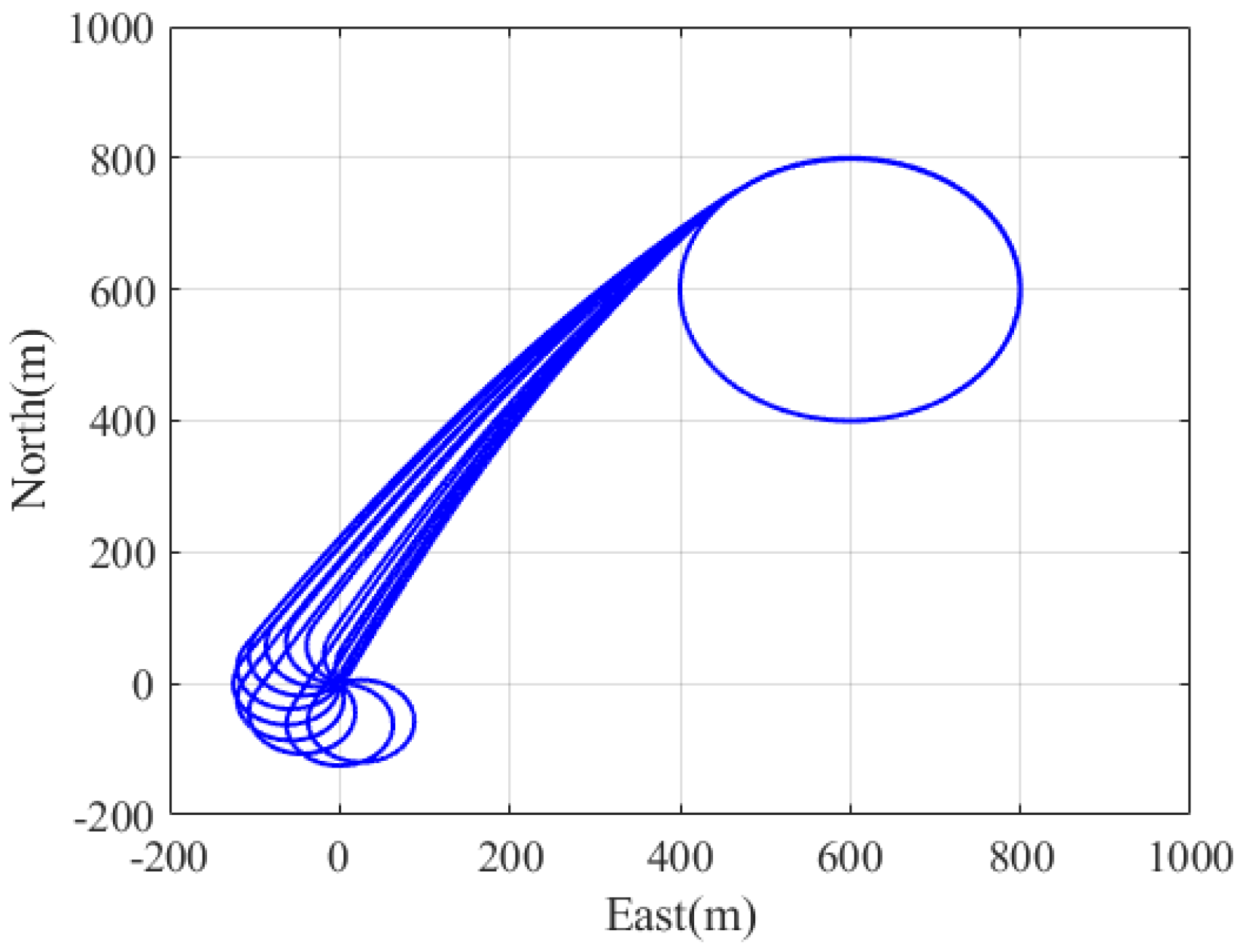
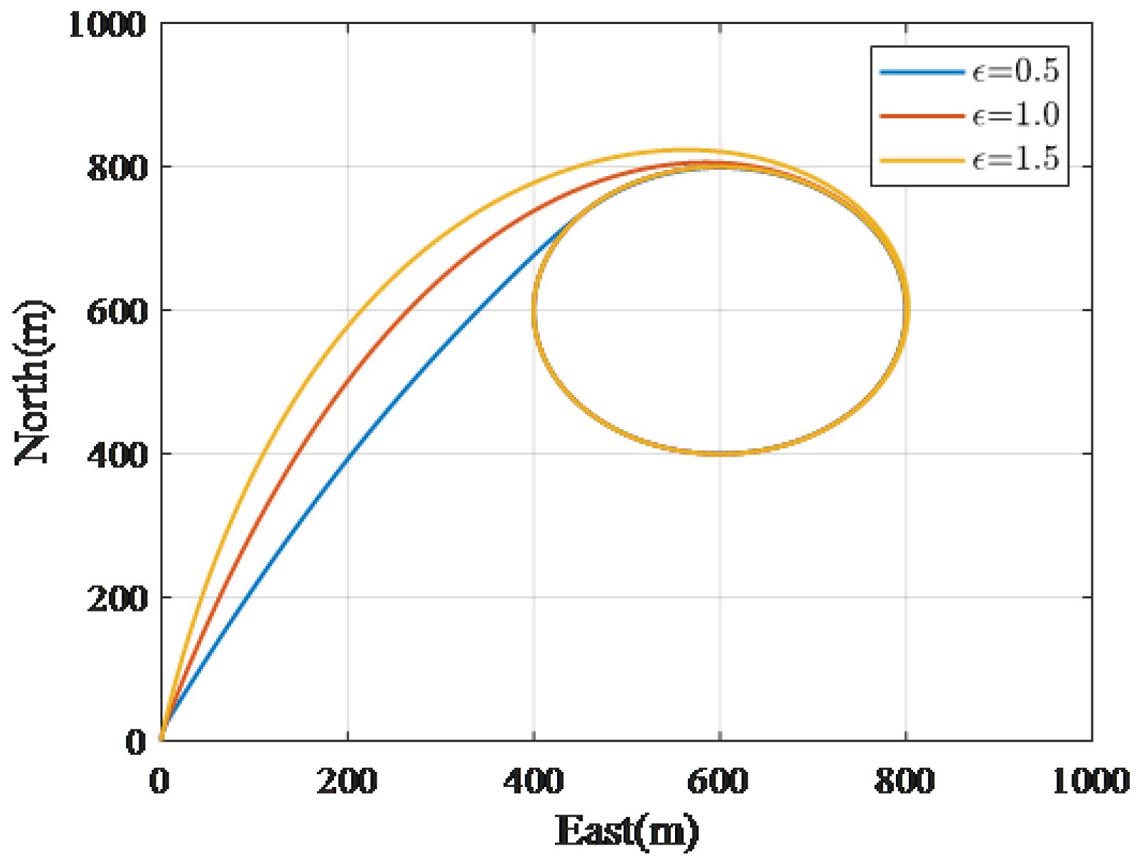
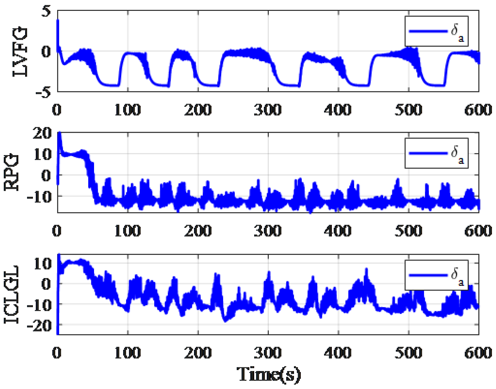
5.2. Target Tracking by ICLGL

The performance of ICLGL is compared with that of LVFG [11] and RPG [28] for tracking a static target. It should be noted that the ICLGL and RPG give the roll angle command signal while the LVFG gives the heading angle command signal. The desired standoff radius is 200 m.

The simulation results of tracking the static target located at $(600\mathrm{m},600\mathrm{m},0\mathrm{m})$ are given in Figure 6 and Figure 7. The simulation results show that RPG and ICLGL converge to circular trajectory faster than LVFG. To show the stability of the ICLGL, we construct simulations under different initial heading conditions. The UAV started with the heading angle of $0^{\circ },22.5^{\circ },{45}^{\circ },\dots ,{360}^{\circ }$ and the results are shown in Figure 8. The results for $\epsilon =0.5,1.0,1.5$ while $k=10$ are shown in Figure 9. We can find that the smaller the value of $\epsilon$, the faster the convergence speed.

Figure 6. Trajectory in horizontal plane.

Figure 7. Horizontal distance between UAV and target.

Figure 8. Simulation with variable initial headings.

Figure 9. Trajectory in the horizontal plane.

5.3. Target Tracking Based on OTSCKF

A six-degree-of-freedom model of the UAV was adopted for this study. The UAV model designed by our laboratory is shown in Figure 10. Table 2 gives the necessary parameters. An autopilot is designed for the model which can realize self-stable attitude control. The start point of the ground target is set to (200 m, 200 m) and the velocity is set to (8 m/s, $4\pi cos(\pi /250\ast t)$ m/s).

Figure 10. The UAV model used in this study.

Table 2. UAV parameters.

Name	Value	Unit
Moment of inertia $I_x$	$4.427$	kg·m${}^2$
Moment of inertia $I_y$	$5.395$	kg·m${}^2$
Moment of inertia $I_z$	$9.361$	kg·m${}^2$
Cruise speed	25	m/s
Take-off mass	$28.875$	kg

Figure 11 shows the trajectory in horizontal plane. From Figure 12, we can find that the RPG and LVFG do not converge to the required tracking radius. When using the LVGF method, UAV will get too close to the target, which is very dangerous. On the other hand, when using ICLGL, the distance can converge to the desired tracking radius. Figure 13 shows the guidance signal and response. From Figure 14 we can find that the deflection of the aileron is within a reasonable range. It should be noted that it takes time for the UAV to respond to the command, the relative distance between the UAVs and the target will oscillate and cannot converge to the expected tracking radius, but the maximum deviation is less than 30 m. In summary, the ICLGL is more accurate and effective in tracking moving targets compared to the LVFG and RPG.

Figure 11. Trajectory in horizontal plane.

Figure 12. Horizontal distance between UAV and target.

Figure 13. Guidance signal and response.

Figure 14. Control surface deflection.

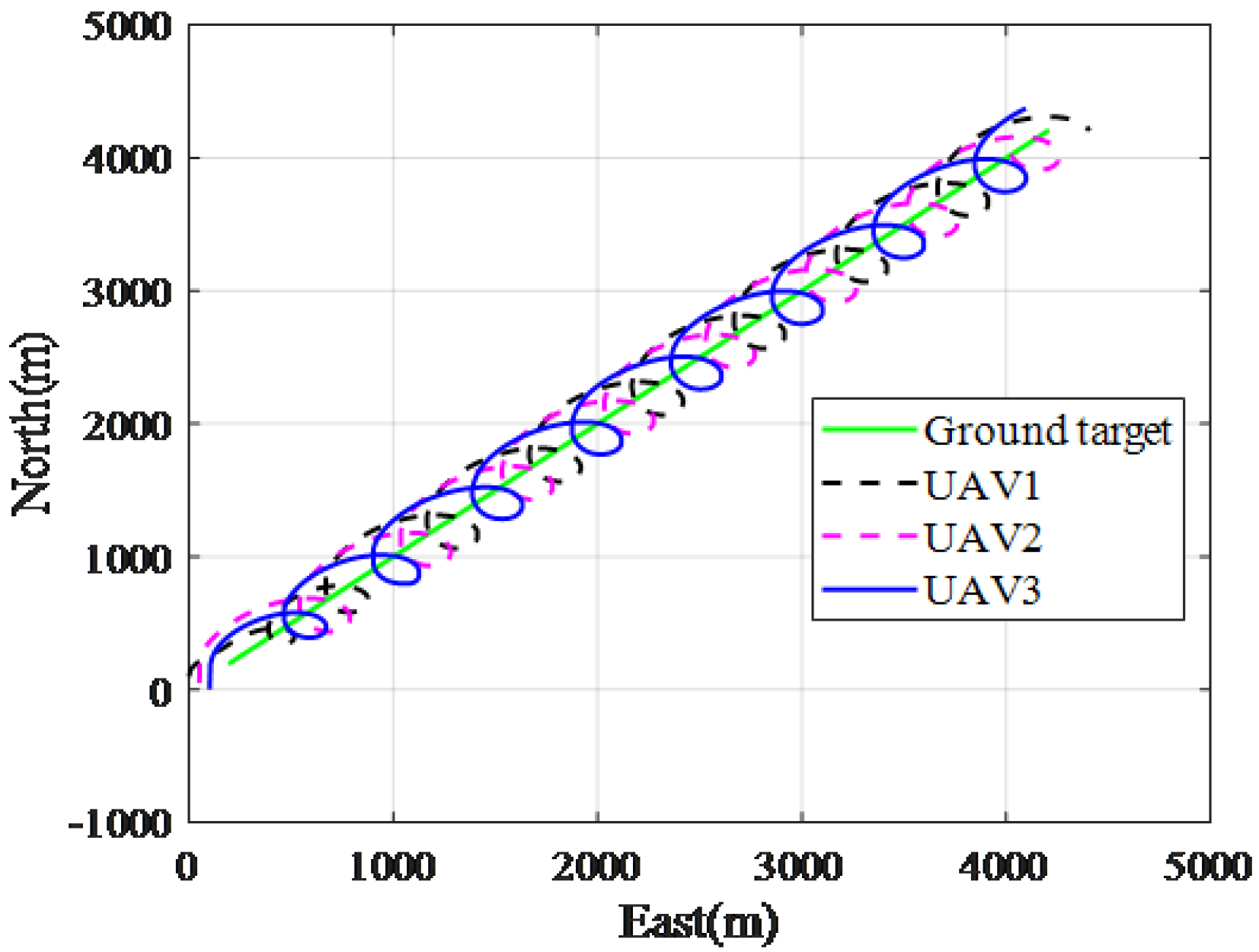
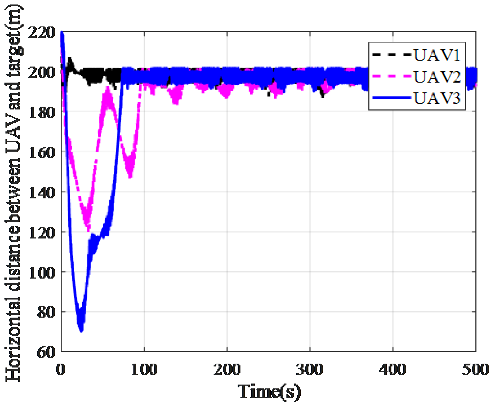
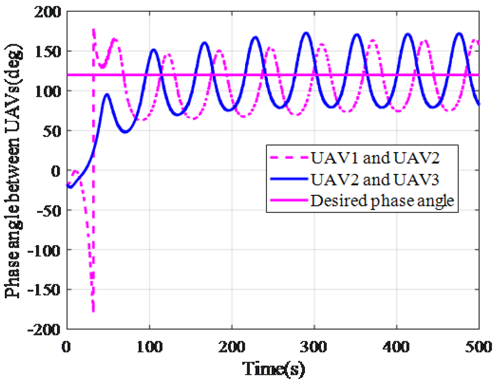
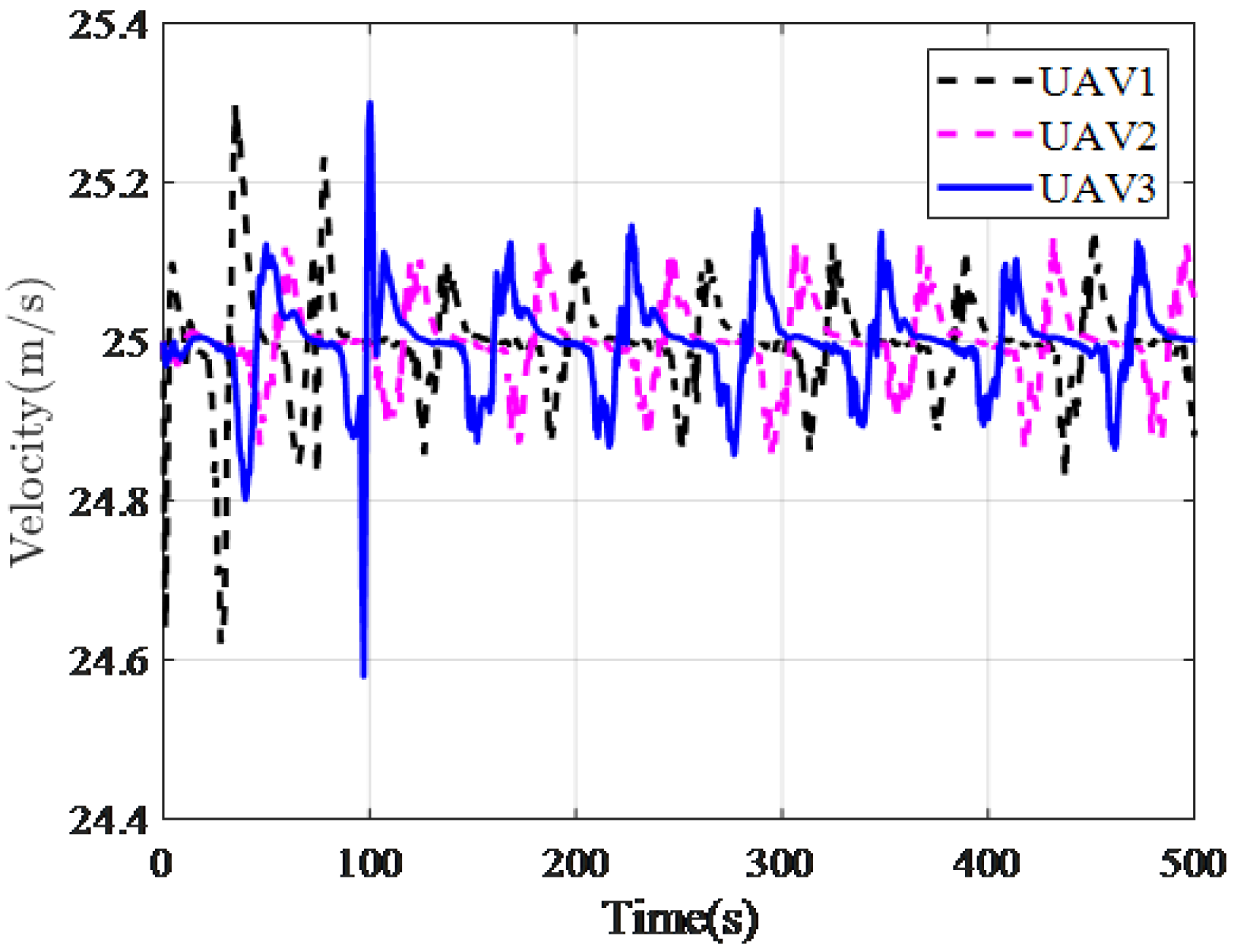
5.4. Coordinated Target Tracking

Given that a target moved along a straight trajectory with the start point (200 m, 200 m, 0 m). Three UAVs performed the mission of target tracking, and the initial positions were (0 m, 0 m, 1000 m), (0 m, 100 m, 1000 m), and (0 m, −100 m, 1000 m), respectively. Figure 15 shows the paths of the UAVs. From Figure 16, we can find that three UAVs converge to the required tracking radius R. Figure 17 shows the deflection of the aileron and Figure 18 shows the phase difference between UAV1, UAV2, and UAV3, which oscillates around the required phase $2\pi /3$. Note that the ICLGL only controls the lateral factor, the velocity and height of three UAVs do not change, as shown in Figure 19 and Figure 20. The simulation results indicate that the coordinated guidance law based on ICLGL can solve the problem of coordinated target tracking.

Figure 15. Paths of the UAVs.

Figure 16. Horizontal distance between UAVs and target.

Figure 17. Deflection of the aileron.

Figure 18. Phase differences.

Figure 19. Velocity.

Figure 20. Height.

From the above discussion, we know that RPG and ICLGL converge to circular trajectory faster than LVFG when tracking stable target. When tracking moving target, only ICLGL can converge to the desired tracking radius. However, the control surface deflection of ICLGL is larger than that of RPG and LVFG. This is the problem that can be optimized in the future.

6. Conclusions

In this paper, the key problems of target tracking of a ground target have been studied. The OTSCKF filter has been designed to estimate the states of the target, which improves the accuracy of target position estimation. The ICLGL guidance law has been proposed to guide the UAVs to conduct standoff tracking of ground moving targets and stability of the algorithm has been proved. The effectiveness of the proposed algorithms in this paper has been verified by simulation. The estimation error of the OTSCKF is less than 10 m and the phase error of the coodinated tracking is less than ${40}^{\circ }$. The results have demonstrated that the estimation method and guidance law perform well considering the existence of noises.

Hardware-In-the-Loop (HIL) simulations can be used to further test the effectiveness of the algorithm and are worthy of further study. The data noise and communication delay in the actual UAV system can not be reflected in the digital simulation. Therefore, to further verify the effectiveness of the algorithm in tracking moving ground targets, HIL simulations are needed. After that, we can carry out the real flight test in order to apply the guidance law in more complex situations.

References

- Ogren, P.; Backlund, A.; Harryson, T.; Kristensson, L.; Stensson, P. Autonomous UCAV Strike Missions Using Behavior Control Lyapunov Functions. In Proceedings of the AIAA Guidance, Navigation, and Control Conference and Exhibit, Keystone, CO, USA, 21–24 August 2006. [Google Scholar]
- Erkan, S.; Kandemir, M.; Giger, G. Advanced task assignment for unmanned combat aerial vehicles targeting cost efficiency and survivability. In Proceedings of the 46th AIAA Aerospace Sciences Meeting and Exhibit, Reno, NV, USA, 7–10 January 2008; p. 873. [Google Scholar]
- Wang, C.Q.; Feng, L.I.; Zhang, J. A survey on UCAV system. Electron. Opt. Control 2004, 9, 41–45. [Google Scholar]
- Lin, C.; Shi, J.; Zhang, W.; Lyu, Y. Standoff tracking of a ground target based on coordinated turning guidance law. ISA Trans. 2022, 119, 118–134. [Google Scholar] [CrossRef] [PubMed]
- Yi, S.; He, Z.; You, X.; Cheung, Y.-M. Single object tracking via robust combination of particle filter and sparse representation. Signal Process. 2015, 110, 178–187. [Google Scholar] [CrossRef]
- He, Q.; Zhang, W.; Huang, D.; Chen, H.; Liu, J. Aircraft Inertial Measurement Unit Fault Diagnosis Based on Optimal Two-Stage CKF. Xibei Gongye Daxue Xuebao/J. Northwest. Polytech. Univ. 2018, 36, 933–941. [Google Scholar] [CrossRef]
- Friedland, B. Treatment of bias in recursive filtering. IEEE Trans. Autom. Control 1969, 14, 359–367. [Google Scholar] [CrossRef]
- Alouani, A.T.; Xia, P.; Rice, T.R.; Blair, W.D. On the optimality of two-stage state estimation in the presence of random bias. IEEE Trans. Autom. Control 1993, 38, 1279–1283. [Google Scholar] [CrossRef]
- Hsieh, C.S.; Chen, F.C. Optimal solution of the two-stage Kalman estimator. IEEE Trans. Autom. Control 1999, 44, 194–199. [Google Scholar] [CrossRef] [Green Version]
- Mashhad, A.M.; Karsaz, A.; Mashhadi, S.K.M. High Maneuvering Multiple-Underwater Robot Tracking with Optimal Two-Stage Kalman Filter and Competitive Hopfield Neural Network Based Data Fusion. Int. J. Commun. Antenna Propag. 2013, 3, 191–198. [Google Scholar]
- Frew, E.W.; Lawrence, D.A.; Morris, S. Coordinated Standoff Tracking of Moving Targets Using Lyapunov Guidance Vector Fields. J. Guid. Control Dyn. 2008, 32, 290–306. [Google Scholar] [CrossRef]
- Hong, J.; Kim, Y.; Bang, H. Cooperative circular pattern target tracking using navigation function. Aerosp. Sci. Technol. 2018, 76, 105–111. [Google Scholar] [CrossRef]
- Park, S.; Deyst, J.; How, J. A new nonlinear guidance logic for trajectory tracking. In Proceedings of the AIAA Guidance, Navigation, and Control Conference and Exhibit, Providence, RI, USA, 16–19 August 2004; pp. 1–18. [Google Scholar]
- Lee, J.Y.; Kim, H.G.; Kim, H.J. Adjustable impact-time-control guidance law against non-maneuvering target under limited field of view. Proc. Inst. Mech. Eng. Part G J. Aerosp. Eng. 2021, 236, 368–378. [Google Scholar] [CrossRef]
- Park, S. Circling over a Target with Relative Side Bearing. J. Guid. Control Dyn. 2016, 39, 1450–1456. [Google Scholar] [CrossRef]
- Park, S. Guidance Law for Standoff Tracking of a Moving Object. J. Guid. Control Dyn. 2017, 40, 2948–2955. [Google Scholar] [CrossRef]
- Cao, Y. UAV circumnavigating an unknown target using range measurement and estimated range rate. In Proceedings of the 2014 American Control Conference, Portland, ON, USA, 4–6 June 2014; pp. 4581–4586. [Google Scholar]
- Cao, Y.C. UAV circumnavigating an unknown target under a GPS-denied environment with range-only measurements. Automatica 2015, 55, 150–158. [Google Scholar] [CrossRef] [Green Version]
- Wise, R.A.S.; Rysdyky, R.T. UAV Coordination for Autonomous Target Tracking. In Proceedings of the AIAA Guidance, Navigation, and Control Conference and Exhibit, Keystone, CO, USA, 21–24 August 2006; p. 6453. [Google Scholar]
- Quintero, S.; Copp, D.A.; Hespanha, J.P. Robust UAV coordination for target tracking using output-feedback model predictive control with moving horizon estimation. In Proceedings of the 2015 American Control Conference (ACC), Chicago, IL, USA, 1–3 July 2015; pp. 3758–3764. [Google Scholar]
- Adamey, E.; Ozguner, U. A decentralized approach for multi-UAV multitarget tracking and surveillance. Int. Soc. Opt. Photonics 2012, 8389, 307–312. [Google Scholar]
- Moseley, M.B.; Grocholsky, B.P.; Cheung, C.; Singh, S. Integrated long-range UAV/UGV collaborative target tracking. In Unmanned Systems Technology XI; International Society for Optics and Photonics: Bellingham, WA, USA, 2009; Volume 7332, p. 733204. [Google Scholar]
- Cui, X.; Jing, Z.; Luo, M.; Guo, Y.; Qiao, H. A new method for state of charge estimation of lithium-ion batteries using square root cubature Kalman filter. Energies 2018, 11, 209. [Google Scholar] [CrossRef] [Green Version]
- Nourmohammadi, H.; Keighobadi, J. Decentralized INS/GNSS system with MEMS-grade inertial sensors using QR-factorized CKF. IEEE Sens. J. 2017, 17, 3278–3287. [Google Scholar] [CrossRef]
- Liu, X.; Liu, X.; Zhang, W.; Yang, Y. Interacting multiple model UAV navigation algorithm based on a robust cubature Kalman filter. IEEE Access 2020, 8, 81034–81044. [Google Scholar] [CrossRef]
- Zhao, X.; Lin, W.; Hao, J.; Zuo, X.; Yuan, J. Clustering and pattern search for enhancing particle swarm optimization with Euclidean spatial neighborhood search. Neurocomputing 2016, 171, 966–981. [Google Scholar] [CrossRef]
- LaSalle, J.P. Stability of nonautonomous systems. Nonlinear Anal. Theory Methods Appl. 1976, 1, 83–90. [Google Scholar] [CrossRef]
- Park, S.; Deyst, J.; How, J.P. Performance and Lyapunov stability of a nonlinear path following guidance method. J. Guid. Control Dyn. 2007, 30, 1718–1728. [Google Scholar] [CrossRef]
Publisher’s Note: MDPI stays neutral with regard to jurisdictional claims in published maps and institutional affiliations. |
© 2022 by the authors. Licensee MDPI, Basel, Switzerland. This article is an open access article distributed under the terms and conditions of the Creative Commons Attribution (CC BY) license (https://creativecommons.org/licenses/by/4.0/).