Article

Predicting Taxi-Calling Demands Using Multi-Feature and Residual Attention Graph Convolutional Long Short-Term Memory Networks

1
State Key Laboratory of Resources and Environmental Information System, Institute of Geographic Sciences and Natural Resources Research, Chinese Academy of Sciences, Beijing 100101, China
2
University of Chinese Academy of Sciences, Beijing 100049, China
*
Author to whom correspondence should be addressed.
ISPRS Int. J. Geo-Inf. 2022, 11(3), 185; https://doi.org/10.3390/ijgi11030185
Submission received: 20 January 2022 / Revised: 5 March 2022 / Accepted: 7 March 2022 / Published: 9 March 2022

Abstract

:
Predicting taxi-calling demands at the urban area level is vital to coordinate the supply–demand balance of the urban taxi system. Differing travel patterns, the impact of external data, and the expression of dynamic spatiotemporal demand dependence pose challenges to predicting demand. Here, a framework using residual attention graph convolutional long short-term memory networks (RAGCN-LSTMs) is proposed to predict taxi-calling demands. It consists of a spatial dependence (SD) extractor, which extracts SD features; an external dependence extractor, which extracts traffic environment-related features; a pattern dependence (PD) extractor, which extracts the PD of demands for different zones; and a temporal dependence extractor and predictor, which leverages the abovementioned features into an LSTM model to extract temporal dependence and predict demands. Experiments were conducted on taxi-calling records of Shanghai City. The results showed that the prediction accuracies of the RAGCN-LSTMs model were a mean absolute error of 0.8664, a root mean square error of 1.4965, and a symmetric mean absolute percentage error of 43.11%. It outperformed both classical time-series prediction methods and other deep learning models. Further, to illustrate the advantages of the proposed model, we investigated its predicting performance in various demand densities in multiple urban areas and proved its robustness and superiority.

1. Introduction

Building an effective, intelligent transportation system by realizing effective traffic resource allocation is one of the important goals of developing cities. To meet such a requirement, it is critical to gain insight into travel demands and conduct accurate forecasting. Taxi services, a popular means of travel, can reflect dynamic changes in travel demands of different regions in a city. Online taxi-calling services not only help travelers to find available taxis more efficiently, but also help city managers to conduct informed traffic planning and resource scheduling, to alleviate traffic congestion, and to reduce the unnecessary use of public resources.
Urban traffic travel is a multi-dimensional and complex dynamic interactive behavior which is affected by many factors, such as environment, economy, and society, and these factors have been discussed [1,2,3]. Due to the intrinsic and dynamic time-space dependence of taxi-calling demands, it is difficult to forecast taxi-calling demands accurately and robustly. In recent years, several studies regarding taxi demands, and related temporal, spatial, and external relationships, have been conducted. Among them, the widely used autoregressive integrated moving average (ARIMA) [4] and its variants [5] have been the most representative time series prediction methods. Further, spatial relationships have been considered by some studies [6,7]. In addition, several studies [8,9,10] have introduced traffic environment information (weather, air quality, events, etc.) into their prediction models. Although these studies show that prediction can be improved by considering additional factors, it presents new challenges, such as finding ways to express complex spatiotemporal and external relations in the model.
In recent years, deep neural networks (DNNs) have been adopted to predict taxi-calling demands [10,11,12,13] by capturing these complex relationships. The graph convolutional neural network (GCN) has attracted attention for its capacity to extract spatiotemporal and semantic correlations of data. However, the main difference between travel patterns in various city functional areas and the spatiotemporal dependence of external factors results presents challenges to DNN-based methods. These include:
  • Semantic relationships in the expression of pattern dependence (PD). Different city functional areas have various travel patterns. The semantic information is related to the taxi-calling demands; thus, it needs to be considered in modeling.
  • Spatiotemporal relationship in the expression of external factors. Several external factors have certain spatiotemporal dependence. A prediction model should not only consider the relationship between external factors and taxi-calling demands, but also consider the spatiotemporal dependence of the external factors themselves.
Based on the graph attention network model [14], GatedGCN [15] introduces the residual idea of the ResNet model to extract deeper features. Inspired by the GatedGCN model, this study constructs a model based on residual attention graph convolutional long short-term memory networks (RAGCN-LSTMs) to integrate temporal, spatial, external, and pattern dependence. The RAGCN-LSTMs model is composed of four modules. The first module extracts spatial dependence (SD) for each functional area with the GatedGCN by modeling the spatial relationship of different depths of taxi-calling demands. The second module retrieves external dependence (ED) from open web texts with a linear convolution model. The third module identifies the PD with an embedding method. Then, the time dependence (TD) of the dependences is extracted with an LSTM [16] model and integrated to predict the taxi-calling demands at the next moment.
The main contributions of this work are:
  • The idea of PD is introduced into taxi-calling demand forecasting with a graph representation learning method.
  • A unified framework is proposed to integrate spatial, temporal, external, and PD for taxi-calling demands’ modeling.
  • It is proved that PD improves the accuracy and robustness of taxi-calling demands prediction, and that the RAGCN-LSTMs model is superior to other state-of-the-art models.

2. Related Works

Several methods have been presented on taxi-calling demands prediction. These methods are grouped into three categories: statistical methods, traditional machine learning (ML) methods, and deep learning (DL) methods.
Statistical methods adopt temporal series analysis to forecast taxi-calling demands. This method is used for its operational efficiency and ease of deployment. Moreira-Matias et al. [5] proposed the aggregation of GPS signals into histogram time series and use the Poisson and autoregressive moving average models to predict demand. Li et al. [17] used ARIMA to predict the number of passengers in the upcoming interval.
Traditional ML methods explore and simulate human learning mechanisms to predict the demand for taxis. Chiang et al. used the Poisson process and Gaussian mixture model to cluster the spatiotemporal points [18]. Li et al. proposed a short-term traffic demand forecasting model (Wave SVM) by combining wavelet analysis and least squares support vector machines (LS-SVM) [19]. Mukai et al. applied a multilayer perceptron (MLP) to predict taxi-calling demands [20]. Zhao et al. even used three predictors to adapt to different resolutions of regions [21].
Statistical and traditional ML methods are difficult to capture the nonlinear relationships between data in most cases, and DL methods make up for this defect. Some mainstream DL models have been applied to taxi-calling demands prediction. For example, long-term short-term memory (LSTM) [16] networks (a variant of the Recurrent Neural Network [RNN]) have been used in prediction work and sometimes even combine with convolutional neural networks (CNN) models. CNN models are firstly used to obtain spatial features, which are then inputted into an RNN model to obtain spatiotemporal features for prediction. Yao et al. proposed a deep multi-view spatiotemporal network (DMVST-Net), which uses CNN and LSTM to extract spatial, semantic, and temporal features to predict taxi-calling demands [22]. Liu et al. proposed a contextualized spatiotemporal network (CSTN) based on ConvLSTM and CNN, which uses similar features to predict taxi origin-destinations (ODs) [13]. Duan et al. proposed a hybrid deep network model (OD-TGAT) based on ConvLSTM to predict taxi ODs [23]. The above methods have made significant contributions to taxi-calling demands prediction.
Graph neural networks (GNNs) deal with non-Euclidean data that is difficult to deal with using CNNs. At present, research on graph signals is divided into two categories: the spatial and frequency domain methods [24]. The latter became increasingly popular after Kipf and Welling proposed the graph convolutional network (GCN) [25,26,27,28]. Huang et al. propose Diffusion Convolutional Recurrent Neural Network (DCRNN) to predict the traffic flow, which can capture the spatial dependency using bidirectional random walks on the graph, and the temporal dependency using the encoder-decoder architecture [29]. Xiao et al. use spatiotemporal graph convolutional networks (ST-GCN) to predict the demands of the shared bikes [30]. However, when there are too many convolution layers, it is equivalent to global low-pass filtering. Attention and residual mechanisms, the two most influential mechanisms in DL, have also been introduced into GNNs. Veličković et al. calculated the normalized attention of each central vertex on different neighbors to improve GNN performance of classification tasks [14]. To solve problems related to low-pass filtering in deep layers of GNN models, Bresson et al. introduced the residual mechanism into the GNN model and constructed the GatedGCN model to improve the number of trainable layers in the model [15]. This allowed deep features to be obtained and improved prediction accuracy. Our model is inspired by the GatedGCN.

3. Preliminary Steps

3.1. Region Partition

It was often necessary to divide the geographical space in geographical spatiotemporal prediction. There were three common division methods: the first was based on different levels of urban road networks; the second used a grid to divide (i.e., rectangular, hexagon, etc.), of which the rectangular grid was most common, as rectangular grids were used to organize data; the third method used existing data on urban area division, such as administrative boundaries, urban functional areas, and urban postcodes. Here, the third method was used, because the same types of urban functional areas often had similar travel pattern and taxi demand, and the other two methods broke the integrity of urban functional areas.

3.2. City Graph

For an urban functional areas map M ( R ) (simplified urban land use type map), where R = { R 1 , R 2 , , R N } were city functional areas, we abstracted each functional area into a vertex and connected adjacent functional areas with edges. The corresponding city graph was defined as G = ( V , E ) , where the vertex set V = { v 1 , v 2 , , v N } represented city functional areas. Edge set E = { e 1 , e 2 , , e M } indicated the connection between the functional areas. Because some functional areas did not generate taxi-calling orders, they were not considered in the city map.

3.3. Prediciting Taxi-Calling Demands

For urban functional area map M ( R ) and time interval t , the corresponding city graph was G = ( V , E ) . For any vertex v k V , the corresponding functional area in city functional zoning map M ( R ) was R k . For vertex v k , taxi-calling demanded at period t was defined as X t v k :
S t v k = { P ( l o c ,     p t ) }
X t v k = N U M ( S t v k )
where l o c and p t respectively represented the location and time of a taxi-calling demand P , and S t v k was the set of taxi-calling demands in vertex v k during time interval t . The function N U M (   ) counted the number of elements in a set.
Taxi-calling demands prediction aimed to forecast the demands of all vertices in the city graph in the next period by using historical taxi-calling data. For a given city graph V = { v 1 , v 2 , , v N } , current time interval t , time interval step s , historical taxi-calling demands X, and dependent characteristics C (time, spatial characteristics, weather, etc.). The taxi-calling demands of next period t + 1 was as follows:
X t + 1 = { X t + 1 v 1 , X t + 1 v 2 , , X t + 1 v N }  
= F ( X t s , X t s + 1 , , X t , C t s , C t s + 1 , , C t )
where F (   ) was the prediction function and the time interval step s was the number of recent historical periods participating in forecasting in time interval t + 1 .

4. Materials and Methods

We designed a RAGCN-LSTMs model based on the advantages of GatedGCN and LSTM. The RAGCN-LSTMs model will be described in detail in this section.

4.1. Overview of the Framework

The RAGCN-LSTMs model consisted of four modules (Figure 1): SD was used to express the SD of taxi-calling demands; ED was used to express the impact of weather, air quality, and other environmental factors on taxi-calling demands; PD was adopted to represent the impact of functional area type on taxi-calling demands; and TD combined the output features of ED, PD, and SD, and input them into the LSTMs to obtain prediction results.

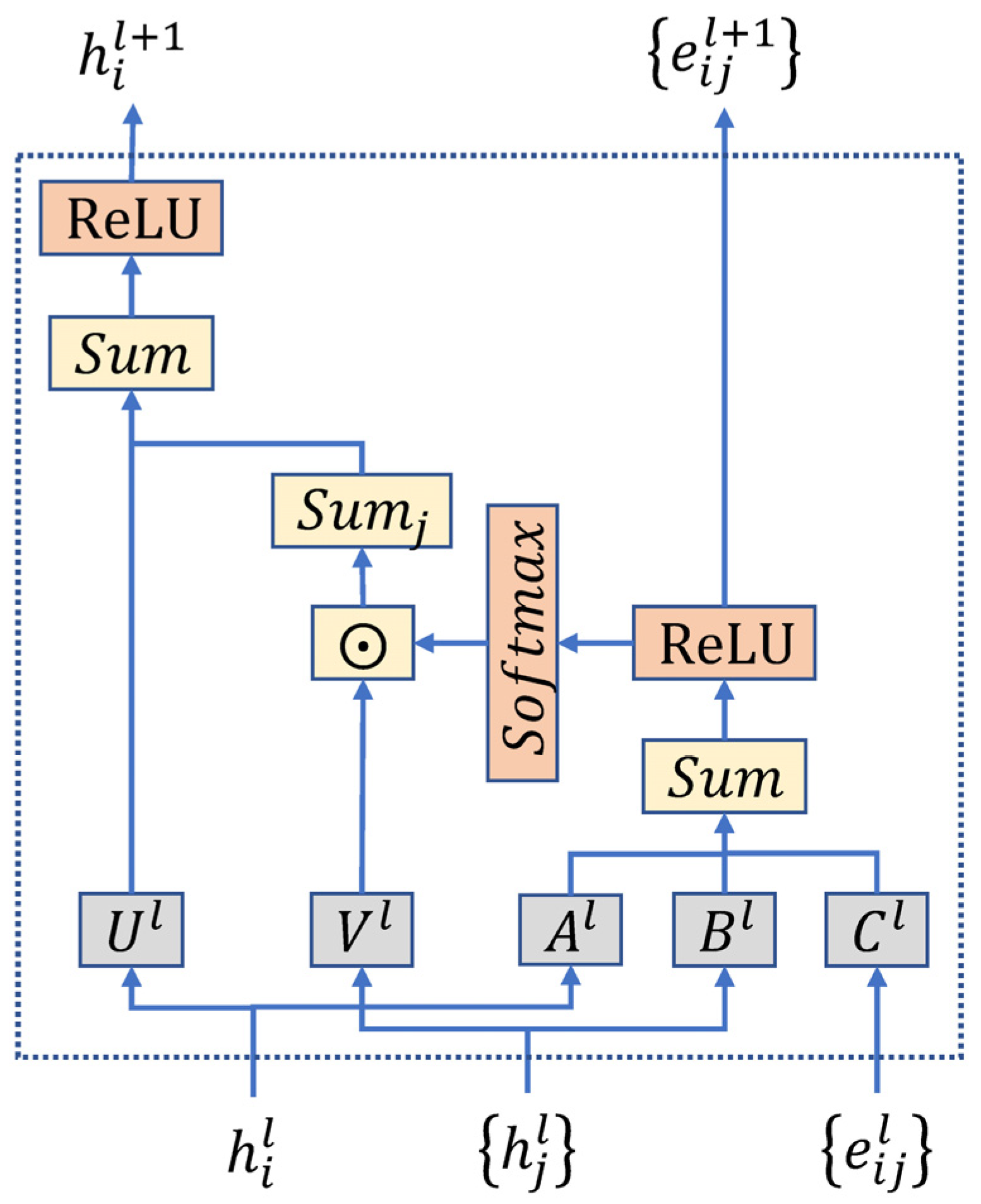
4.2. Extracting Spatial Feature

We transformed the city functional zoning map into city graph G , and filled the current time interval features (vectors of taxi-calling demands) of functional areas into the vertices of G . Vertex v i had vertex features h i . The GatedGCN’s goal was to help update the features of each vertex under the influence of neighbors (see, Figure 2).
GatedGCN designed an anisotropic GCN by considering residual join, batch normalization, and edge gates. The update formula of edge gates and vertex features was:
h i l + 1 = h i l + R e L U ( B N ( U l h i l + j N i e i j l V l h i l ) )
where U l , V l d × d were weight matrices, ⊙ was the Hadamard product, ReLU() was an activation function, and BN() was Batch Normalization layer, the edge gates e i j l was defined as:
e i j l = σ ( e ^ i j l ) j σ ( e ^ i j l ) + ε
e ^ i j l = e ^ i j l 1 + R e L U ( B N ( A l h i l 1 + B l h j l 1 + C l e ^ i j l 1 )
Here, σ was a sigmoid function, ε was a very small correction constant (for computational stability), and A l , B l , C l d × d were weight matrices, and l was the l - th layer of GatedGCN. The output result h l a s t of the last layer was the feature vector τ ( S ) = h l a s t of SD.

4.3. Extracting External Feature

The ED feature extraction module consisted of a convolution layer. The externally dependent factors (such as weather, temperature, wind speed, and air quality) were standardized. Among them, the quantitative data (such as weather description) were standardized by max-min value, and textual data (such as weather description) were heat coded (one-hot coding), after which the standardized vectors were combined. The feature vector of ED τ ( E ) was obtained using a convolution layer as follows:
τ ( E ) = C A T ( C 1 , C 2 , , C l ) W E
where the function C A T ( ) was the combined operation function, C i was the external dependent factor after standardization, and W E was the weight matrix.

4.4. Extracting Pattern Feature

The more comparable the functional area types were, the more uniform the public travel patterns would be. Therefore, we encoded the functional area categories of the vertices in the city graph G = ( V , E ) with the classical embedding representation method. This allowed us to obtain the pattern feature vector τ ( P ) as:
τ ( P ) = λ · e m b e d d i n g ( F v k ) + ( 1 λ ) e m b e d d i n g ( v k )
Among them, the function e m b e d d i n g (   ) was the embedding representation function, F v k was the functional area type of vertex   v k V , λ was a parameter that needed training, e m b e d d i n g ( F v k ) represented the embedding representation of vertex v k V functional area type, and e m b e d d i n g ( v k ) represented the embedding representation of vertex v k V in the Graph G .
In this way, not only the quantitative expression of each vertex functional area, but also the quantitative expression included the relationship between vertex categories in the graph.

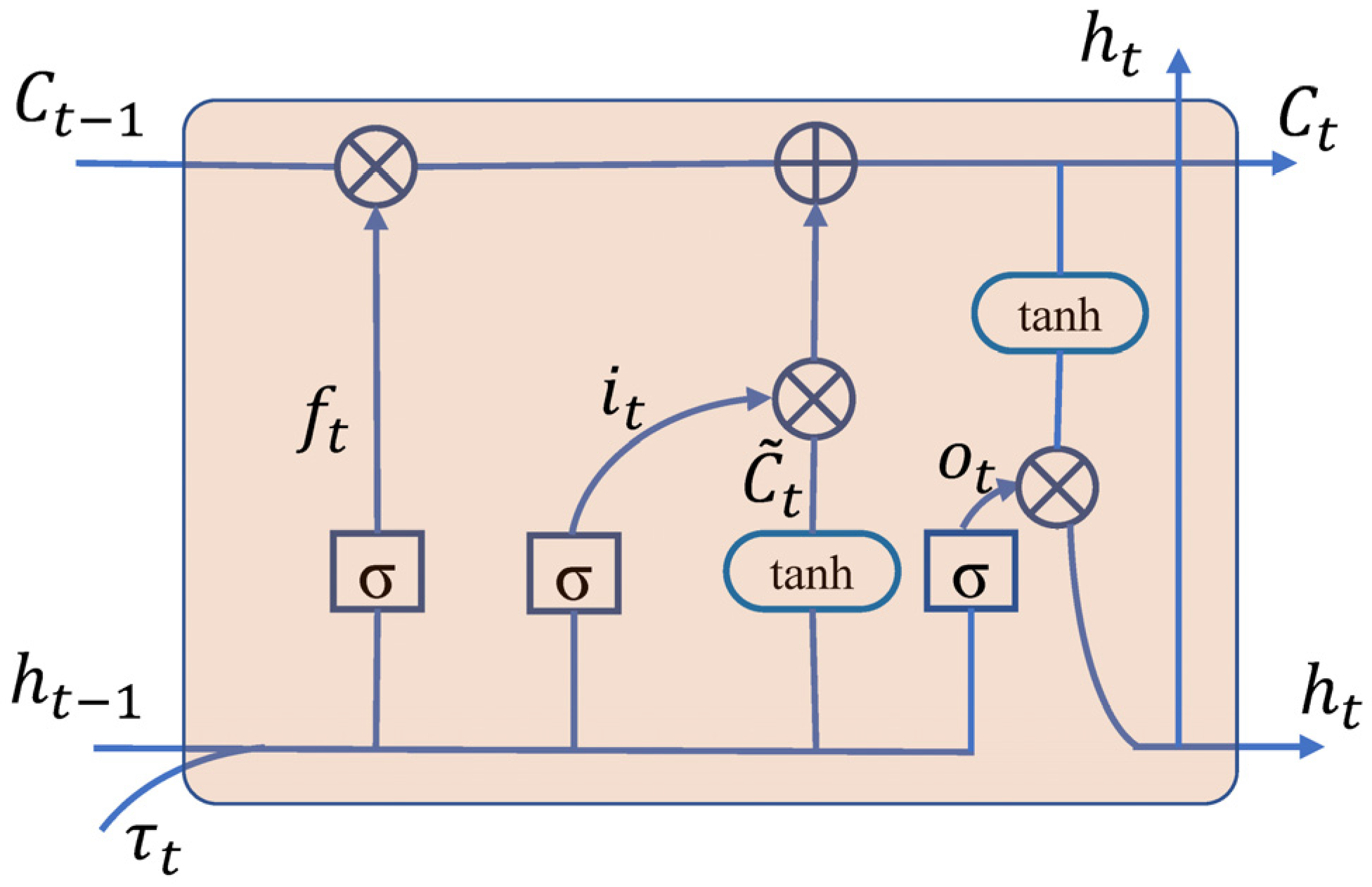
4.5. Temporal Feature Extraction

The time feature module combined acquired features, analyzed the time series, and predicted taxi-calling demands for the next moment. We used an LSTM model for the time series as follows. The external eigenvectors obtained were τ ( E ) , the spatial eigenvector was τ ( S ) , and mode eigenvectors were τ ( P ) . Then, these were combined to obtain the total eigenvector τ , following which the total eigenvectors at different times were input into the LSTMs module to obtain forecast results for the next period.
Figure 3 shows the structure of each cell in the LSTM model. In time interval t , the total eigenvector τ t and the previous hidden h t 1 were input. The hidden state h t was calculated as:
f t = σ ( W f [ h t 1 , τ t ] + b f )
i t = σ ( W i [ h t 1 , τ t ] + b i )
C ˜ t = t a n   h ( W c [ h t 1 , τ t ] + b C )
C t = C t 1 f t + i t C ˜ t
o t = σ ( W o [ h t 1 , τ t ] + b o )
h t = o t t a n   h ( C t )
where W and b denoted the corresponding weights and bias vectors; τ t , h t and C t represented the input, output and memory cells at time interval t ; h t 1 and C t 1 represented the output and memory cells at time interval t 1 ; i t , o t and f t were the input, output and forget gates.
The last layer of the LSTMs generated hidden state h t s . After calling the full connection layer, the taxi-calling demanded of all vertices in city graph G at t + 1 interval was obtained.
X t + 1 = R e L U ( W h t s + b )

5. Results and Discussion

5.1. Experiment Setup

5.1.1. Datasets

A real taxi-calling dataset for Shanghai which was provided by Shanghai Johnson & Johnson Intelligent Navigation Technology Co., Ltd., in Shanghai of China from 1 to 30 April 2014 and other related data were used in the experiment. We extracted taxi ODs from the trajectory records and collected the corresponding meteorological information for Shanghai from the same period, that was acquired from the meteorological data center of China Meteorological Administration (http://data.cma.cn/, 26 December 2021). As most taxi trips began downtown, we chose the Huangpu District (one of the central city areas in Shanghai) as the research area. A land use dataset of the Huangpu District from the end of 2013 obtained from Shanghai Municipal Bureau of planning and natural resources was collected. The three data sets were described as:
  • Taxi OD dataset. Each original taxi trajectory record contained information such as time stamp, geographic coordinates, and taxi operating status. After excluding the trips whose departure and destination were not in the research area, we ended up with 1.8 million taxi-calling orders. Finally, according to the time stamp and geographical coordinates of the taxi trip records, the taxi number in each functional area was counted, and the taxi departure demanded matrix in each time interval was generated. In this dataset, each time interval was set to 30 min.
  • Meteorological information. Meteorological information of Shanghai was collected from an authorized meteorological agency with the frequency of 30 min. We considered the effects of temperature, humidity, wind speed, air pressure, and weather conditions in our study. Among them, precipitation level information and air quality level information were included in the weather conditions. Table 1 shows the overview of meteorological information in research areas. The one-hot code was used to digitize the weather conditions, and the other four numerical indicators were normalized to [0,1] range. Finally, the meteorological information in t time interval was expressed as vector M t n (see, Table 1).
  • Land use dataset: Different city functions could be reflected by land use types. Figure 4 shows the land use map of the research area as, wherein 10 types were presented. We merged and abridged some areas (such as water bodies, green belts, etc.) where it was almost impossible to have taxi-calling orders.

5.1.2. Baselines

The proposed method was compared to the following methods because, to achieve the best performance, the parameters of all methods were adjusted.
Historical average (HA): The taxi demands of each region in the next period was forecasted by averaging the historical taxi demands of the same period.
Autoregressive integrated moving average (ARIMA) [17]: Moving average and autoregressive components were combined to build time correlation model.
Multiple layer perceptron (MLP) [20]: A neural network consisted of four fully connected layers with 2048, 1024, 512, and 282 neurons, respectively. The order demand data of T pre-time intervals in the function area was used as the input of the MLP model, and the output was the order demand of the next time interval.
Long short-term memory (LSTM) [16]: A variant of RNN, it learned potential long and short-term dependencies from sequence data.
Diffusion convolution recurrent neural network (DCRNN) [29]: Graph convolution was integrated into the gating cycle unit for spatiotemporal prediction. In this model, the two-way graph random walk operation is used to extract spatial dynamic features, and RNN was used to obtain temporal dynamic features.
Spatiotemporal graph convolutional network (ST-GCN) [30]: Composed of several ST-Conv blocks, which were constructed with fully convoluted layers to deal with the task of spatiotemporal series prediction. Specifically, each block was composed of graph convolution and gated time convolution to process graph structured time series.
The performance of different modules in the model was analyzed to study its effectiveness in taxi-calling demands prediction.

5.1.3. Metrics

We used three indicators to compare all methods: mean absolute error (MAE), root mean square error (RMSE) and symmetric mean absolute percentage error (SMAPE):
M A E = 1 z t = 1 z Y t Y ^ t
R M S E = 1 z t = 1 z Y t Y ^ t 2
S M A P E = 1 z t = 1 z Y t Y ^ t ( Y t + Y ^ t ) / 2
where z was the total number of test samples, Y ^ t and Y t was the predicted taxi-calling demands of time interval t and the corresponding ground truth value. The input and output of our proposed network were normalized to the range [0,1] during the training process. Therefore, in the evaluation, we scaled the predicted value to the normal value, and then compared it with the true value.

5.1.4. Default Setting

The data used for the experiments spans 30 days. A total of 80% of the data (23 days) was used for training (among them, 10% of randomly selected training data was used for validation), and the remaining 20% (7 days) was used for testing. The model was implemented with PyTorch (version 1.8.0 + cu111) and ran on NVIDIA GTX 1080Ti.
Each timed interval t was 30 min; the length of the whole time series being 1440, which is also the number of all intervals. After that, the step size was set to 20, so in each time interval, features from the past 20 intervals were used to predict the next interval. In terms of network parameters, GatedGCN and LSTM had five and two layers, respectively. In model training, parameter update optimizer used the Adam optimizer and Loss function used L1 loss, and the learning rate decayed from 1.0 × 10⁻³ to 1.0 × 10⁻⁵ at 0.5 times.

5.2. Comparison with Baselines

Table 2 shows the prediction performance of our RAGCN-LSTMs model, and other methods for taxi-calling demanded prediction. RAGCN-LSTMs achieved the best performance among all the methods. Specifically, in terms of MAE, RMSE and SMAPE, RAGCN-LSTMs had improved by 2.003%, 3.769%, and 2.994% compared with the best baseline model (ST-GCN), respectively. Additionally, HA and ARIMA performed poorly (MAE was 1.1552 and 1.0461, RMSE was 2.0531 and 1.8731, and SMAPE was 52.86% and 49.29%, respectively), which might be due to their dependence on historical demand. Compared with the traditional neural network method, MLP performed better, which indicate that it found further nonlinear correlation. Additionally, DCRNN and ST-GCN performed well, especially in MAPE and RMSE, which proved that they had strong expression ability for spatiotemporal dependence. However, their performance was still not as good as that of the RAGCN-LSTMs model, which proved the validity of the latter.

5.3. Evaluating Modules

By inputting different dependence features into the model, we evaluated the effectiveness of different module’s features (see, Table 3). Each module in the model could make it better. By comparing the results of TD (LSTM) and SD + TD, we confirmed the value of SD. SD improved the prediction accuracy greatly, accounting for 51.19%, 42.43%, and 49.94% of the improvement in MAE, RMSE, and SMAPE, respectively. Adding an ED module based on SD + TD could further improve the model’s prediction accuracy of the model. Through the comparison between SD + ED + TD, and all the dependencies, the effectiveness of the correlation between the functional areas extracted by PD for predicting taxi-calling demands was verified.

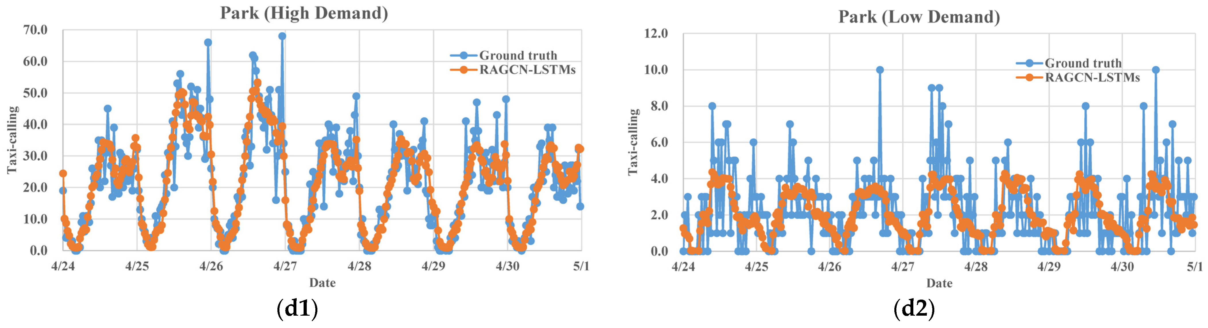
5.4. Evaluating Functional Area Prediction Results

Further, to verify the robustness of the model, we experimentally verified the prediction accuracy of the model under different typical land use types and different levels of taxi-calling demands. We investigated the prediction accuracies of four land use types: commercial lands, old-fashioned residences, new residences, and parks in high (areas with an average weekly taxi-calling demands greater than 3000 cases) and low demand (about 800 cases) areas (see Figure 5). Specifically, in commercial areas, whether high or low demand areas, (with a few exceptions) the overall prediction results of the model were consistent with the ground truth, as Figure 5(a1,a2) shows. For old residences, the prediction effect of the model was the same as that of the commercial land, as Figure 5(b1,b2) shows. This might be due to the traditional separation of work and residence in commercial areas and old residences. The demand mode of taxi-calling had a relatively stable periodicity, which was captured by our model. As Figure 5(c1,c2) shows, in the new residences, compared with the first two, the prediction accuracy of the model did not change in detail in the high demand area, but decreased in the low demand area. This was because the new residences were planned and constructed to solve the separation of urban work and housing, and there were often workplaces near these residential areas. However, not all residents and staff came from this area. Therefore, in the new residences, the taxi-calling demanded not only had an early peak, but a late peak (in high demand areas, most peaks occurred in the morning, but both morning and evening peaks existed in low demand areas). This made the travel pattern in these areas complex and difficult to predict, especially in low demand areas. In parkland areas, there were no regular morning and evening peaks, and the travel pattern in these areas was complex and difficult to explain. However, our model could capture these complex features and had precise prediction, as Figure 5(d1,d2) shows. Our model achieved precise prediction for all land use types and levels of taxi-calling demands.

5.5. Impacts of Parameters

Additionally, we evaluated the impact of some key parameters of the model, time step and convolution layer depth. Figure 6a shows the RMSE prediction error of relative step size. Our method achieved the best performance when the time was 20. Generally, the RMSE decreased first, then it did not change with an increase in time step, indicating that the time interval of more than 20 had little effect on the demand forecast of next-moment orders. Figure 6b illustrates the performance of the model in terms of the number of convolution layers. When the number of layers was five, the model performed best. As the number of layers continued to increase, the prediction performance of the model began to decline. This might be because, with the increase of convolution layers, the model traversed almost all vertices, and when the number of convolution layers was greater than five, it was unable to extract deeper, useful feature information.

6. Conclusions

In this study, we propose a RAGCN-LSTMs. To explore the relationships between functional areas, we introduced a graph embedding method called PD in RAGCN-LSTMs. On this basis, the graph residual attention neural network was used to extract the features of different depth and neighbor range of each central region. Additionally, by using external features, such as meteorological information, we explored its impact on taxi-calling demand prediction. We evaluated the proposed model on the Shanghai taxi order data set. The experimental results showed that:
(1)
RAGCN-LSTMs had better prediction results than other base models, indicating that it could better capture space-time, pattern, and ED.
(2)
Through the evaluation of different dependence feature modules, PD was one of the most important influencing factors for space-time prediction.
(3)
By analyzing the prediction results of different levels of taxi-calling demands, in various urban functional areas, considering various dependent factors could improve the model’s robustness.
Our model was not only superior to other base models in prediction accuracy but had strong robustness through the experiments in various functional areas with different levels of taxi-calling demand. All these proved that our model had good practicability. For taxi companies, the data required for model prediction could be easily obtained, and there were no other stringent requirements in actual industrial applications.
In future research, we will use more advanced ML models to better express the dependence of taxi-calling demands and introduce geographical laws into the model, such as different spatiotemporal scale characteristics, temporal non-stationarity, and spatial heterogeneity, to solve the problem that sudden peaks are hard to predict and to make the model more interpretable.

Author Contributions

Conceptualization, Chunlei Mi and Feng Lu; methodology, Chunlei Mi and Shifen Cheng; data curation, Chunlei Mi; software, Chunlei Mi; validation, Chunlei Mi, Shifen Cheng and Feng Lu; writing—original draft preparation, Chunlei Mi; writing—review and editing, Feng Lu and Shifen Cheng; visualization, Chunlei Mi; supervision, Feng Lu; funding acquisition, Feng Lu. All authors have read and agreed to the published version of the manuscript.

Funding

This work was supported by the National Natural Science Foundation of China, grant number 42101423 and the China Postdoctoral Science Foundation, grant number 2020M680655 and 2021T140656.

Data Availability Statement

The data are not publicly available due to restrictions on their use imposed by law and the entity collecting the data.

Acknowledgments

We would like to thank all contributing authors and the anonymous reviewers for their valuable inputs and cooperation in this Special Issue.

Conflicts of Interest

The authors declare no conflict of interest.

References

  1. Schwanen, T.; Banister, D.; Anable, J. Scientific research about climate change mitigation in transport: A critical review. Transp. Res. Part A Policy Pract. 2011, 45, 993–1006. [Google Scholar] [CrossRef] [Green Version]
  2. Dingil, A.E.; Rupi, F.; Esztergár-Kiss, D. An Integrative Review of Socio-Technical Factors Influencing Travel Decision-Making and Urban Transport Performance. Sustainability 2021, 3, 10158. [Google Scholar] [CrossRef]
  3. Ewing, R.; Cervero, R. Travel and the built environment: A synthesis. Transp. Res. Rec. 2001, 1780, 87–114. [Google Scholar] [CrossRef] [Green Version]
  4. Shekhar, S.; Williams, B.M. Adaptive Seasonal Time Series Models for Forecasting Short-Term Traffic Flow. Transp. Res. Rec. J. Transp. Res. Board 2007, 2024, 116–125. [Google Scholar] [CrossRef]
  5. Moreira-Matias, L.; Gama, J.; Ferreira, M.; Mendes-Moreira, J.; Damas, L. Predicting Taxi–Passenger Demand Using Streaming Data. IEEE Trans. Intell. Transp. Syst. 2013, 14, 1393–1402. [Google Scholar] [CrossRef] [Green Version]
  6. Deng, D.X.; Shahabi, C.; Demiryurek, U.; Zhu, L.H.; Yu, R.; Liu, Y.; Assoc Comp, M. Latent Space Model for Road Networks to Predict Time-Varying Traffic. In Proceedings of the 22nd ACM SIGKDD International Conference on Knowledge Discovery and Data Mining (KDD), San Francisco, CA, USA, 13–17 August 2016; Association Computing Machinery: San Francisco, CA, USA, 2016; pp. 1525–1534. [Google Scholar] [CrossRef] [Green Version]
  7. Tong, Y.X.; Chen, Y.Q.; Zhou, Z.M.; Chen, L.; Wang, J.; Yang, Q.; Ye, J.P.; Lv, W.F. The Simpler The Better: A Unified Approach to Predicting Original Taxi Demands based on Large-Scale Online Platforms. In Proceedings of the 23rd ACM SIGKDD International Conference on Knowledge Discovery and Data Mining (KDD), Halifax, NS, Canada, 13–17 August 2017; Assoc Computing Machinery: Halifax, NS, Canada, 2017; pp. 1653–1662. [Google Scholar] [CrossRef]
  8. Pan, B.; Demiryurek, U.; Shahabi, C. Utilizing Real-World Transportation Data for Accurate Traffic Prediction. In Proceedings of the 12th IEEE International Conference on Data Mining (ICDM), Brussels, Belgium, 10–13 December 2012; IEEE: Brussels, Belgium, 2012; pp. 595–604. [Google Scholar] [CrossRef] [Green Version]
  9. Wu, F.; Wang, H.J.; Li, Z.H. Interpreting Traffic Dynamics using Ubiquitous Urban Data. In Proceedings of the 24th ACM SIGSPATIAL International Conference on Advances in Geographic Information Systems (ACM SIGSPATIAL GIS), San Francisco, CA, USA, 31 October–3 November 2016; Association Computing Machinery: San Francisco, CA, USA, 2016; pp. 1–4. [Google Scholar] [CrossRef]
  10. Xu, Y.; Li, D. Incorporating Graph Attention and Recurrent Architectures for City-Wide Taxi Demand Prediction. ISPRS Int. J. Geo-Inf. 2019, 8, 414. [Google Scholar] [CrossRef] [Green Version]
  11. Chen, Z.; Zhao, B.; Wang, Y.; Duan, Z.; Zhao, X. Multitask Learning and GCN-Based Taxi Demand Prediction for a Traffic Road Network. Sensors 2020, 20, 3776. [Google Scholar] [CrossRef] [PubMed]
  12. Tang, J.; Liang, J.; Liu, F.; Hao, J.; Wang, Y. Multi-community passenger demand prediction at region level based on spatio-temporal graph convolutional network. Transp. Res. Part C Emerg. Technol. 2021, 124, 102951. [Google Scholar] [CrossRef]
  13. Liu, L.; Qiu, Z.; Li, G.; Wang, Q.; Ouyang, W.; Lin, L. Contextualized Spatial–Temporal Network for Taxi Origin-Destination Demand Prediction. IEEE Trans. Intell. Transp. Syst. 2019, 20, 3875–3887. [Google Scholar] [CrossRef] [Green Version]
  14. Veličković, P.; Cucurull, G.; Casanova, A.; Romero, A.; Lio, P.; Bengio, Y. Graph attention networks. arXiv 2017, arXiv:1710.10903. [Google Scholar]
  15. Bresson, X.; Laurent, T. Residual gated graph convnets. arXiv 2017, arXiv:1711.07553. [Google Scholar]
  16. Hochreiter, S.; Schmidhuber, J. Long short-term memory. Neural Comput. 1997, 9, 1735–1780. [Google Scholar] [CrossRef] [PubMed]
  17. Li, X.L.; Pan, G.; Wu, Z.H.; Qi, G.D.; Li, S.J.; Zhang, D.Q.; Zhang, W.S.; Wang, Z.H. Prediction of urban human mobility using large-scale taxi traces and its applications. Front. Comput. Sci. 2012, 6, 111–121. [Google Scholar] [CrossRef]
  18. Chiang, M.-F.; Hoang, T.-A.; Lim, E.-P. Where are the passengers? a grid-based gaussian mixture model for taxi bookings. In Proceedings of the 23rd SIGSPATIAL International Conference on Advances in Geographic Information Systems, Seattle, WA, USA, 3–6 November 2015; pp. 1–10. [Google Scholar] [CrossRef]
  19. Li, Y.; Lu, J.; Zhang, L.; Zhao, Y. Taxi booking mobile app order demand prediction based on short-term traffic forecasting. Transp. Res. Rec. 2017, 2634, 57–68. [Google Scholar] [CrossRef]
  20. Mukai, N.; Yoden, N. Taxi demand forecasting based on taxi probe data by neural network. In Intelligent Interactive Multimedia: Systems and Services; Springer: Berlin/Heidelberg, Germany, 2012; pp. 589–597. [Google Scholar] [CrossRef]
  21. Zhao, K.; Khryashchev, D.; Freire, J.; Silva, C.; Vo, H. Predicting Taxi Demand at High Spatial Resolution: Approaching the Limit of Predictability. In Proceedings of the 4th IEEE International Conference on Big Data (Big Data), Washington, DC, USA, 5–8 December 2016; IEEE: Washington, DC, USA, 2016; pp. 833–842. [Google Scholar] [CrossRef]
  22. Yao, H.; Wu, F.; Ke, J.; Tang, X.; Jia, Y.; Lu, S.; Gong, P.; Ye, J. Deep Multi-View Spatial-Temporal Network for Taxi Demand Prediction. In Proceedings of the AAAI Conference on Artificial Intelligence, New Orleans, LA, USA, 2–7 February 2018; Volume 32, pp. 2588–2595. [Google Scholar]
  23. Duan, Z.T.; Zhang, K.; Chen, Z.; Liu, Z.Y.; Tang, L.; Yang, Y.; Ni, Y.Y. Prediction of City-Scale Dynamic Taxi Origin-Destination Flows Using a Hybrid Deep Neural Network Combined With Travel Time. IEEE Access 2019, 7, 127816–127832. [Google Scholar] [CrossRef]
  24. Dwivedi, V.P.; Joshi, C.K.; Laurent, T.; Bengio, Y.; Bresson, X. Benchmarking graph neural networks. arXiv 2020, arXiv:2003.00982. [Google Scholar]
  25. Rukmanda, T.D.; Sugeng, K.A.; Murfi, H. Modification of Architecture Learning Convolutional Neural Network for Graph. In Proceedings of the 3rd International Symposium on Current Progress in Mathematics and Sciences (ISCPMS), Faculty Mathematics & Natural Sciences, University Indonesia, Bali, Indonesia, 26–27 July 2017; American Institute of Physics Inc.: Bali, Indonesia, 2017. [Google Scholar] [CrossRef]
  26. Tran, D.V.; Navarin, N.; Sperduti, A. On Filter Size in Graph Convolutional Networks. In Proceedings of the 8th IEEE Symposium Series on Computational Intelligence (IEEE SSCI), Bengaluru, India, 18–21 November 2018; IEEE: Bengaluru, India, 2018; pp. 1534–1541. [Google Scholar] [CrossRef] [Green Version]
  27. Jiang, B.; Zhang, Z.Y.; Lin, D.D.; Tang, J.; Luo, B.; Soc, I.C. Semi-supervised Learning with Graph Learning-Convolutional Networks. In Proceedings of the IEEE/CVF Conference on Computer Vision and Pattern Recognition (CVPR), Long Beach, CA, USA, 16–20 June 2019; IEEE: Long Beach, CA, USA, 2019; pp. 11305–11312. [Google Scholar] [CrossRef]
  28. Gao, H.C.; Pei, J.; Huang, H.; Assoc Comp, M. Conditional Random Field Enhanced Graph Convolutional Neural Networks. In Proceedings of the 25th ACM SIGKDD International Conference on Knowledge Discovery & Data Mining (KDD), Anchorage, AK, USA, 4–8 August 2019; Association Computing Machinery: Anchorage, AK, USA, 2019; pp. 276–284. [Google Scholar] [CrossRef]
  29. Huang, Y.; Weng, Y.; Yu, S.; Chen, X. Diffusion Convolutional Recurrent Neural Network with Rank Influence Learning for Traffic Forecasting. In Proceedings of the 18th IEEE International Conference on Trust, Security and Privacy in Computing and Communications/13th IEEE International Conference on Big Data Science And Engineering (TrustCom/BigDataSE), Rotorua, New Zealand, 5–8 August 2019; IEEE: Berkeley, CA, USA, 2019; pp. 678–685. [Google Scholar] [CrossRef]
  30. Xiao, G.; Wang, R.; Zhang, C.; Ni, A. Demand prediction for a public bike sharing program based on spatio-temporal graph convolutional networks. Multimed. Tools Appl. 2020, 80, 22907–22925. [Google Scholar] [CrossRef]
Figure 1. Framework of the RAGCN-LSTMs model.
Ijgi 11 00185 g001
Figure 2. Structure of the GatedGCN layer.
Ijgi 11 00185 g002
Figure 3. Structure of the LSTM unit.
Ijgi 11 00185 g003
Figure 4. Land use map of research area.
Ijgi 11 00185 g004
Figure 5. Accuracies of the model predicting taxi-calling demand in areas with different functions. (a1,a2) respectively show the prediction accuracies of high demand area and low demand area in commercial lands; (b1,b2) Old residences; (c1,c2) New residences; (d1,d2) Parks.
Ijgi 11 00185 g005aIjgi 11 00185 g005b
Figure 6. Performance on parameters with different values. (a) Performance on different time step values. (b) Performance on different layer numbers.
Ijgi 11 00185 g006
Table 1. Overview of meteorological information in research area.
TypeInformation
Temperature (°C)5–31
Wind speed (mph)0–27
Humidity (%)12–100
Air Pressure (in)29.4–30.4
WeatherSpecies (sunny, rainy, cloudy, etc.)
Table 2. Performance comparison with baseline models.
ModelHAARIMAMLPLSTMDCRNNST-GCNOurs
MAE1.15521.04610.93020.91250.89100.88520.8664
RMSE2.05311.87311.60211.59031.56111.54761.4965
SMAPE(%)52.8649.2947.5545.0544.3844.0143.11
Table 3. Evaluating modules.
FeaturesMAERMSESMAPE(%)
RAGCN-LSTMs (TD, LSTM) 0.91251.590345.05
RAGCN-LSTMs (SD + TD)0.88891.550544.12
RAGCN-LSTMs (SD + ED + TD)0.87051.515843.45
RAGCN-LSTMs (all dependence)0.86641.496543.11
Publisher’s Note: MDPI stays neutral with regard to jurisdictional claims in published maps and institutional affiliations.

