Abstract
Waterway traffic monitoring is an important content in waterway traffic management. Taking into account that the number of monitored water areas is growing and that waterway traffic management capabilities are insufficient in the current situation in China, this paper investigates the location optimization of the vessel traffic service (VTS) radar station. During the research process, radar attenuation and environmental occlusion, as well as variable coverage radius and multiple covering are all considered. In terms of the radar attenuation phenomenon in the propagation process and obstacles such as mountains and islands in the real world, judgment and evaluation methods in a three-dimensional space are proposed. Moreover, a bi-objective mathematical model is then developed, as well as a modified adaptive strategy particle swarm optimization algorithm. Finally, a numerical example and a case are given to verify the effectiveness of the proposed methods, model, and algorithm. The results show the methods, model, and algorithm proposed in this paper can solve the model efficiently and provide a method to optimize the VTS radar station location in practice.
1. Introduction
The rapid development of maritime transportation has increased the number of vessels operating on waterways. By 2020, China already has 131,555 civil transport vessels, comprising 121,440 motorized vessels and 10,115 barges [1,2]. As a result, the number of accidents involving waterway traffic is increasing as well. For instance, there were 137 waterway traffic accidents in China in 2019, resulting in 155 fatalities or disappearances and 46 shipwrecks, with a direct economic loss of 179.87 million CNY (about US $27.84 million) [2]. To ensure the safety of sailing ships, maritime authorities have increasingly relied on vessel traffic services (VTS) to regulate marine traffic [3]. The International Maritime Organization and the International Association of Marine Aids to Navigation and Lighthouse Authorities have defined vessel traffic service as a shore-based facility that monitors sailing ships and ensures maritime safety through the use of communication facilities such as automatic identification system, radar station, closed-circuit television, and very high frequency. Typically, a VTS system comprises a VTS control center and several or multiple VTS radar stations. China currently has approximately 50 VTS centers and 200 VTS radar stations [2]. In general, in China, regional marine bureaus run and maintain the VTS system is operated. Regional marine bureaus can use the VTS center to effectively propagate information to radar stations, ensuring the safety of ship navigation. According to the Maritime Traffic Safety Law of the People’s Republic of China, the Marine Environmental Protection Law of the People’s Republic of China, and the Safety Supervision and Management Rules for the VTS System of the People’s Republic of China, each regional marine bureaus proposes corresponding safety supervision and management rules for the VTS system, which regulate ship behaviors in a variety of areas, including ship reporting, ship traffic management, and ship safety. Furthermore, pertinent policies, guidelines, and punitive measures are issued. However, as the number and size of sailing ships used in waterway transportation increases, current VTS systems are insufficient to meet monitoring demands, and it is critical to build more VTS systems to meet the rapidly developing needs. Because the VTS system mainly relies on the radar station to track ships, the location of the radar station has a considerable impact on the system’s overall efficiency and effectiveness [4]. As a result, it is vital to conduct research into VTS radar station optimization to enhance the capability of the system to ensure ship navigation safety.
However, obstacles in the real-world geography environment, such as forests, islands, and mountains, will occlude the transmission of electromagnetic waves emitted by VTS radar, affecting the radar’s monitoring performance. This phenomenon is referred to as environmental occlusion in this study. Additionally, electromagnetic waves appear attenuated when they propagate through substances such as water and air, affecting the monitoring performance of the VTS radar. These two factors are considered in the location optimization process in this study. As a result, the following three questions will be addressed in this paper:
How can the attenuation of the electromagnetic waves be measured, and what is the attenuation tendency as the distance between them changes?
How can we determine whether the environmental occlusion occurs or not, and how can we evaluate an environmental occlusion?
How should the location of the VTS radar station be optimized?
To solve these questions, this paper proposes methods for attenuation evaluation and environmental occlusion judgment. To begin with, the attenuation function is introduced to evaluate the influence of the attenuation phenomenon. Then the environmental occlusion judgment method is investigated by spatial geometry in mathematics, which is achieved in a three-dimensional coordinated system. Furthermore, a bi-objective mathematical model is constructed, and a modified adaptive strategy particle swarm optimization (ASPSO) algorithm is designed to solve this model. Moreover, a numerical example is provided to demonstrate the effectiveness of the proposed methods, model, and algorithm. The following sections are organized as follows. Section 2 reviews the related literature. In Section 3, we outline the problem and proposed methods. Section 4 contains an introduction to the algorithm. Section 5 employs a numerical example to test and verify. Finally, Section 6 summarizes the conclusions and further research direction.
2. Related Works
To our knowledge, there are few studies on the optimal location of the VTS radar station. Nevertheless, more efforts on vessel traffic service systems from a variety of perspectives are ongoing. In addition, in essence, the result of VTS radar station location optimization is deciding to locate a set of radar stations subject to some constraints and objective functions. As a result, the problem studied in this paper is similar to a facility location problem (FLP). Moreover, we will give a quick overview of connected works from these two perspectives.
Publications about vessel traffic service systems can be classified into those about the VTS system and those about the VTS operators. VTS is a public service facility dedicated to enhancing social welfare. Initially, numerous pieces of research focused on the demands and outcomes of VTS development, as well as benefit-cost analyses [5]. Then to strengthen VTS supervision capabilities, additional studies focus on adding systems or equipment to VTS or designing systems based on VTS. Kao, Lee, Chang, and Ko [6] and Su, Chang, and Cheng [7] offered a novel vessel collision avoidance choice approach by utilizing a VTS collision alert system. Tsou. Cheng, M. [8,9] used data mining techniques, data warehouse techniques, and online analytical process technologies to improve VTS’s analysis and decision-making capabilities, as well as to provide maritime traffic managers with helpful strategic planning resources. Yet, as the number of ships and vessel traffic flow grows, the VTS systems already built may be insufficient to meet current marine safety regulatory criteria, and further research is conducted on how to lead the development of VTS [10]. Related works on VTS operators focus on the operator’s work content and performance [11,12,13,14], as well as the operator’s work situation [15]. Even if the operators of a single VTS perform admirably, a single VTS system is insufficient to produce a high-level supervision effect throughout the entire sea region. As a result, a collaboration between operators in different VTS or between operators and captains must be explored [16,17]. Additionally, as vessel traffic flow increases, VTS operators will be required to conduct increasingly sophisticated and frequent operations to ensure maritime safety. Therefore, more studies are focusing on operator fatigue induced by onerous work [18], operator cognitive workload assessment [19], and adaptive rotating shift for operators [20] to alleviate the stressful working environment caused by increasing vessel traffic flow. Generally, radar works by emitting electromagnetic waves and detecting those reflected by the monitored object. When electromagnetic waves travel through complex environments, they cause propagation processes such as reflection, refraction, bypassing, and scattering [21]. Given the stochastic nature of the electromagnetic waves propagation mechanism, researchers have developed a range of propagation models for the accurate prediction of radio wave propagation. Electromagnetic wave propagation models usually fall into three categories: fully empirical models, semi-empirical and semi-deterministic models, and deterministic models [22]. Fully empirical models are those based on empirical data. Due to the limited number of factors employed, these models are straightforward but not very precise. Moreover, usually fully empirical models are applied in the macro-cellular environment. These include the Hata and Okumura models, as well as the COST-231 Hata fashion model [23,24,25,26]. On the other hand, deterministic models are extremely precise. Ray Tracing and the Ikegami model are two examples [27,28,29]. Semi-empirical and semi-deterministic models incorporate both empirical data and deterministic elements. Cost-231 Walfisch–Ikegami model is a semi-empirical model [30]. All of these models estimate the mean path loss based on parameters like the transmitter’s and receiver’s antenna heights, the distance between them, and so on. These models have been rigorously evaluated in the context of mobile networks. The majority of these models are constructed through a methodical evaluation of measurement data collected within the service region.
Facility location problems involve selecting the ideal location or location combination for facilities [31]. There were many applications in the previous study, including warehouses, distribution centers, and emergency supplies [32]. Moreover, large quantities of location models have been proposed. According to the principle of location technique, the problems in these publications can be categorized into p-medium problems, p-center problems, and covering problems [33]. Given that radar works in a circular pattern, it seems sensible to incorporate a covering location model into the planning of VTS radar stations. Moreover, there are two types of covering problems: set coverage problems and maximum coverage problems. While under the circumstance of an unlimited number of facilities, the former seeks complete coverage or a certain percentage to cover demand points, under the circumstance of a restricted number of facilities, the latter seeks maximum coverage to cover demand points [34]. Furthermore, many facility location issues based on the coverage model have been investigated. To optimize the location of the three levels of maternity hospitals found in France, Baray and Cliquet [35] provide a hierarchical location-allocation model that combines a maximum covering model and p-center models. Based on the set covering model, Vieira, Ferrari, and Ribeiro, et al. [36] determined the appropriate number and position of counting stations to cover a road network to obtain traffic flows. A variety of calculating methods and algorithms have been developed to solve the models mentioned above. Heuristic algorithms and precise techniques are the two types [37]. Genetic algorithm (GA) [38], particle swarm optimization (PSO) [39], and ant colony optimization algorithm (ACO) are examples of heuristic algorithms. Lagrangian relaxation, branch and bound, Bender’s decomposition method, and more exact solution algorithms are available [40].
As can be observed, there is a shortage of research on VTS radar station location optimization, the majority of papers relevant to vessel traffic service are devoted to VTS systems and operators. Given that the VTS radar station location optimization problem is likewise a facility location problem, this paper adopts the covering model to study the location optimization problem. However, most facility location problems are solved in two-dimensional space, therefore, contributions to the existing literature are made from the following areas.
- A method for judging environmental occlusion induced by obstacles in three-dimensional space is proposed.
- A method for evaluating radar attenuation in three-dimensional space is proposed.
- Taking into account the fact that radar works in a circular pattern, a VTS radar station location optimization model is constructed based on the coverage model.
3. Problem Description
This section discusses the problem of VTS radar station location planning. As discussed previously, environmental occlusion and radar attenuation have a significant impact on the location planning decision. Hence, the evaluation methods of environmental occlusion and radar attenuation are also proposed in this section.
3.1. Problem Description
The VTS radar operates by releasing the electromagnetic wave and capturing the wave reflected by the corresponding monitored water area to perform the monitoring function. Given the fact that VTS radar stations are often located outdoors, this paper introduces the Okumura–Hata propagation model to simulate the electromagnetic propagation process of VTS radar stations. In the real world, the effective height of VTS radar base stations and the communication distance is also more consistent with the applicable conditions of the Okumura–Hata propagation model. However, due to the wavelength limitation of electromagnetic waves, any type of VTS radar will have a minimum monitoring radius r and maximum monitoring radius R. When the distance between the VTS radar station and monitored water area is less than or equal to the minimum radius or greater than or equal to the maximum radius, VTS radar is incapable of monitoring objects effectively. Meanwhile, obstacles such as mountains and forests will impair the VTS radar station’s monitoring ability in the real world. Moreover, the electromagnetic wave will appear attenuated when propagating in the air, water, or other substances. In addition, in practice the maritime authorities have different monitoring requirements for different water areas. For example, the particular water area needs to be monitored twice or three times during the process. Hence, this paper investigates the location optimization problem in the presence of environmental obstacles and radar attenuation, while the factors that different types of radar to be configured with different monitoring radius and monitoring requirements are considered. Figure 1 depicts the specific process.
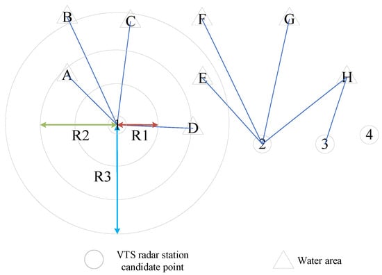
Figure 1.
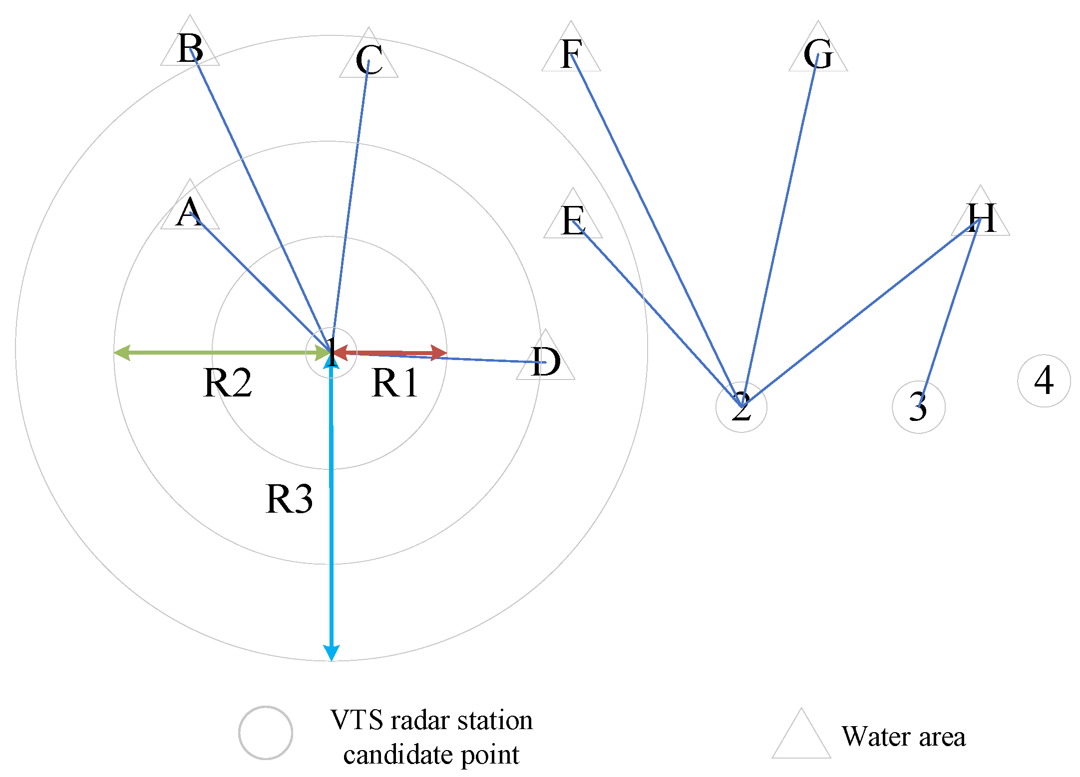
VTS radar station location process.
In Figure 1, circles 1–4 denote potential VTS radar station candidate points, and triangles A–H denote the water areas to be covered. Each VTS radar candidate point is limited to be configured as one type of radar. The configured radar can be chosen from three types in Figure 1, with R1, R2, and R3 denoting the monitoring radius of each type. The purpose of this paper is to select a set of points from the whole VTS candidate points and radar type to fulfill the monitoring requirements about the water area in the presence of environmental obstacles and radar attenuation.
3.2. Radar Attenuation Evaluation
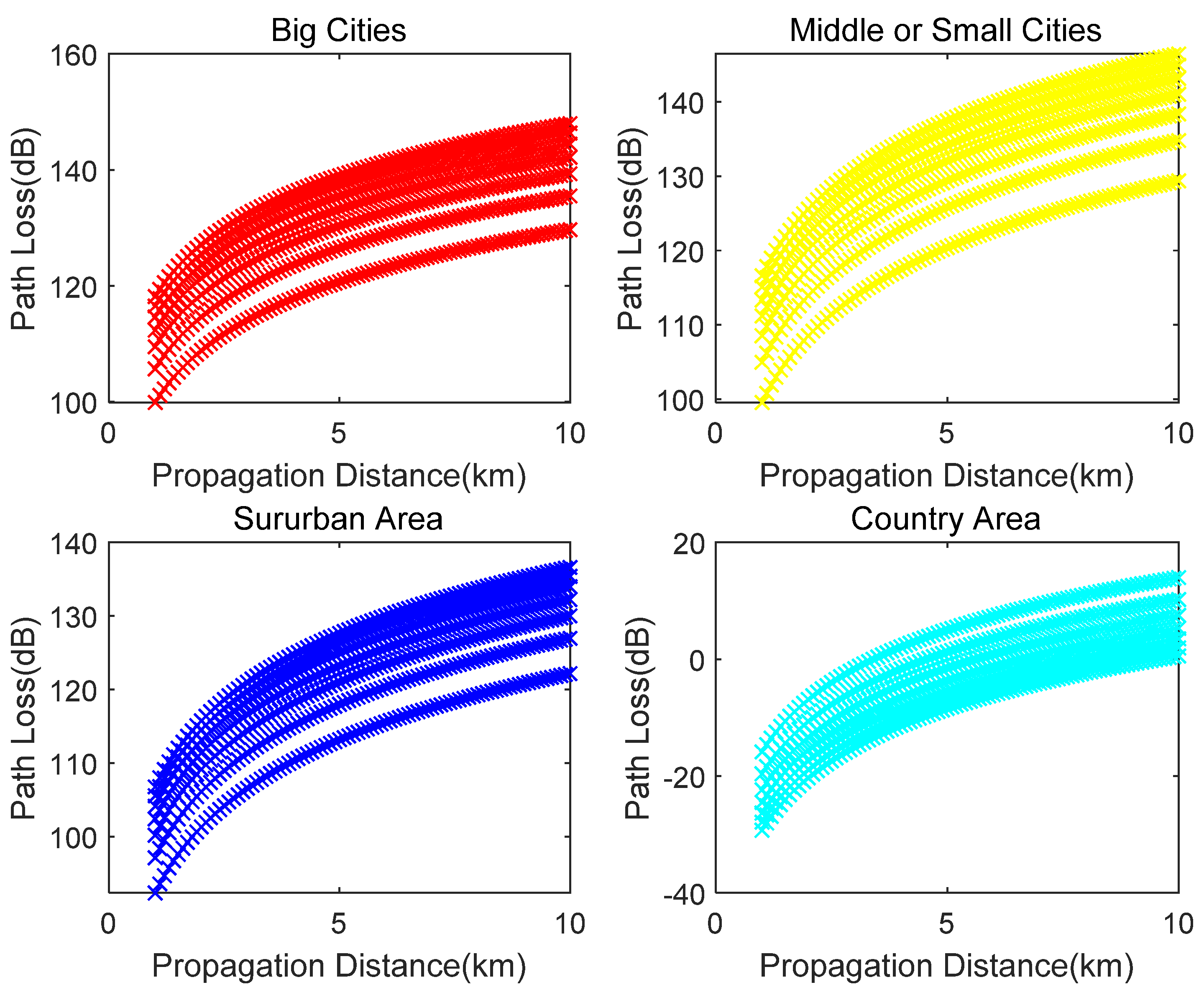
As previously stated, electromagnetic waves appear attenuated when propagating in air and water due to their characteristics. Moreover, the electromagnetic waves’ intensity decreases as the distance between the water area and the radar station grows. To evaluate the degree of radar attenuation, Okumura–Hata’s path loss formulas are introduced to measure the degree of attenuation of electromagnetic waves. The formulas vary according to the geographic scope. Equations (1)–(5) illustrate the specific formulas. In formulas 1–5, the carrier frequency f ranges from 150 Mhz to 1500 Mhz, the distance d between them ranges from 1 km to 20 km, the height of the base station antenna hb ranges from 30 m to 200 m, and the height of mobile antenna hm ranges from 1 m to 10 m. The corresponding variation curves of path loss with propagation distance are shown in Figure 2. It can be seen that the path loss, i.e., radar attenuation, shows a convex increase trend with the propagation distance increases.
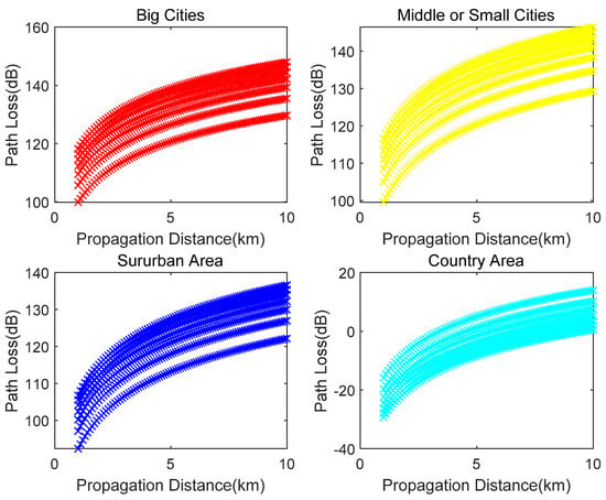
Figure 2.
Variation curve.
One of the paper’s objective functions is to determine the VTS radar station’s coverage rate for the water area, that is, to compute the VTS radar station’s coverage area for the entire monitoring water area as a percentage of the total area. We begin by assuming that the radar station’s coverage rate for the water area is equal to 1 when the water area is within the radar’s monitoring coverage. Moreover, due to electromagnetic wave attenuation, the radar station’s ultimate coverage rate for each water area is equal to 1 minus the attenuation rate. Therefore, the coverage rate of the water area varies between [0, 1]. It is worth noting that Figure 2 depicts the attenuation rate of electromagnetic waves as a logarithmic function with a convex attenuation trend. To facilitate computation, the attenuation function employed in this research is a logarithmic function to determine the attenuation rate, as illustrated in Figure 3.
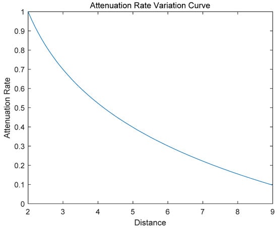
Figure 3.
Attenuation Rate.
Path Loss for urban clutter:
Path loss for suburban clutter:
Path loss for the open country is:
3.3. Environmental Occlusion Judgment and Evaluation Method
When obstacles such as mountains and forests are in the effective monitoring coverage of radar, these obstacles might result in environmental occlusion, impairing the radar’s monitoring effect. Therefore, this factor must be considered in the VTS radar station location planning. This subsection describes the method to judge whether the occlusion exists or not.
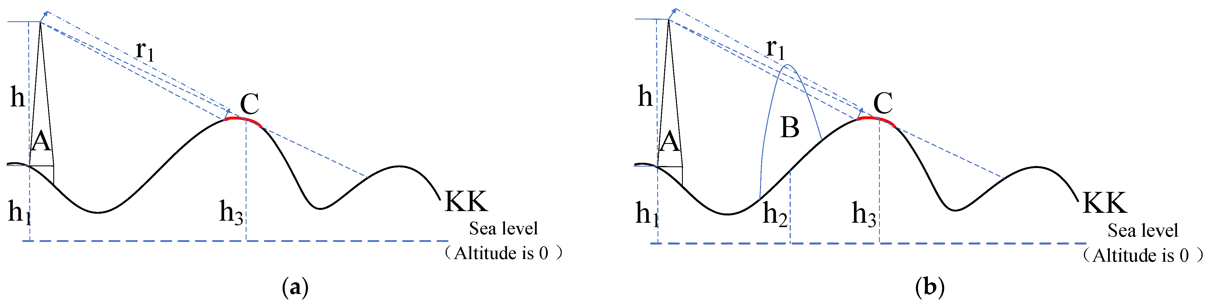
In Figure 4, there are radar station A, obstacle B, and water area C. The corresponding elevations are , , and . The height of each radar station is . The minimum and maximum coverage radius of radar are assumed as and . The Euclidean distance in two-dimensional space between A and C is . Figure 4a depicts the circumstances that there are no obstacles between A and C. The water area C is supposed to be supervised and covered by radar station A when is between and , otherwise it is not. The coverage rate of the radar station is calculated by the radar attenuation function. Figure 4b depicts the circumstances that there is an obstacle B between A and C. We can still judge whether the water area C is supervised and covered as before, but because of the existence of obstacle B, the radar station’s monitoring effect will be affected, and we can know the obstacle B cannot occlude the electromagnetic waves completely in practice, thus this paper assigns different penetration rate to different obstacles. When electromagnetic waves propagate through obstacles in the transmission process, the calculation method of coverage rate of radar station is described as Equation (6). represents the coverage rate of radar station A to water area C when electromagnetic waves do not propagate through obstacle B, calculated by radar attenuation function. is the penetration rate of obstacle B, is the final result of coverage rate of radar station A to water area C in consideration of obstacle B.
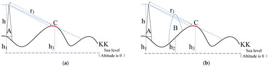
Figure 4.
Environment occlusion in 2-D.
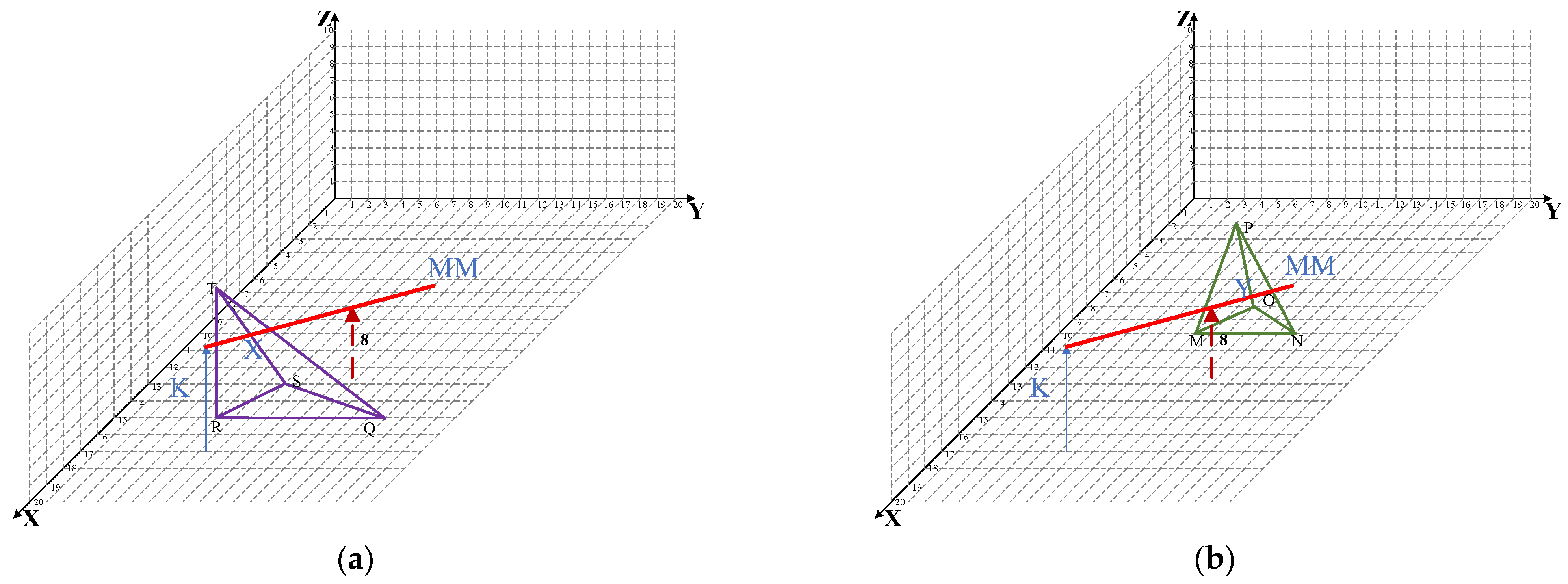
Further, the judgment method of whether the environmental occlusion occurs and coverage rate calculation method are described as follows when the location optimization space becomes a three-dimensional space. Obstacle T-RSQ, VTS radar station K, water area 8, and radar electromagnetic wave MM are shown in Figure 5a. The T-RSQ is a simulation of mountains in a real-world setting. The radar station has its height and geographic elevation, and water area 8 has its elevation as well. When the electromagnetic wave MM passes through the obstacle T-RSQ, the obstacle T-RSQ is considered to generate environmental occlusion when the intersection of the straight-line MM and the cone T-RSQ exists, thus the procedures to determine whether the intersection of MM and T-RSQ exists are described as follows. The first step is to determine whether the straight-line MM is parallel to the four planes represented by T-RSQ, TSQ, TRQ, TRS, and RSQ included. After that, the intersection points are computed and range judgment is carried out. For example, in Figure 5a, when intersection point X exists and comes inside the range of TSQ, TRQ, TRS, or RSQ, environmental occlusion occurs. However, if solely this method is used to judge environmental occlusion, the error indicated in Figure 5b will occur. There is an obstacle P-MON, water area 8, and VTS radar station K in Figure 5b. The intersection point Y is within the range of obstacle P-MON. According to the aforementioned procedure, environmental occlusion occurs. However, it is obvious that there are no obstacles between radar station K and water area 8. Consequently, this research uses the vector inner product measure to rule out this case to correct the environmental occlusion judgment method. At this time the intersection point Y and the water area 8 and the radar station K form vectors and , respectively, when the occlusion is not generated, otherwise it is generated. Moreover, we can adopt the example in Figure 5a to verify the supplementary measure. The occlusion generates because .
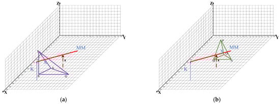
Figure 5.
Environmental occlusion.
The following conditions are utilized to calculate the coverage rate based on the aforementioned foundations. (a) When the water area is not within the radar’s coverage radius, the coverage rate is set to 0. (b) When there is no environmental occlusion and the distance between them is within the coverage radius, the coverage rate is calculated by the attenuation function. (c) When the water area is within the coverage radius and there is environmental occlusion, and the final coverage rate is the product of the attenuation function’s coverage rate and the obstacle’s penetration rate, with the penetration rates of mountains and forests often differing in the real world.
3.4. Mathematical Model
3.4.1. Assumption
- (1)
- External surroundings remain unchanged, which means that the number and elevation of obstacles, water area, and potential VTS radar station candidate points will remain unchanged.
- (2)
- The number, geography area, and elevation of covered water areas are known.
- (3)
- The total number and elevation of potential VTS radar station candidate points are known.
- (4)
- The types and their exact parameters of radar are known, as is the height of the radar station.
- (5)
- The number and penetration rate of obstacles, as well as the formula of attenuation function, are specified in advance.
3.4.2. Problem Formulation
- (1)
- Coverage rate computation
The coverage rate of the VTS radar to the water area is computed by Equation (7), taking into account the presence of obstacles in the surrounding area. Then the coverage rate matrix of the radar station to the entire water areas can be obtained based on Euclidean distance in three-dimensional space.
- (2)
- Area coverage rate calculation
The area coverage rate of each water area is determined by using a parallel approach to obtain the coverage rate matrix, as given in Equation (8).
- (3)
- Model Construction
The bi-objective optimization model developed for the VTS location problem is constructed based on the maximum coverage and set coverage idea and presented in the following.
Objective functions:
Constrains:
The objectives (9) and (10) of Stage 1 are to minimize the total construction cost of the VTS radar station and maximize the area coverage of all water areas, respectively. The total construction cost comprises the fixed construction cost and the configuration cost of radar. Given the maritime authorities’ criteria about the number of times about water area to be covered constraint (11) is set. The area relationship of all water areas is described by Equation (12). Only one type of radar can be configured for each candidate point, as shown in Equation (13). Constraints (14) and (15) are binary decision variable constraints.
4. Algorithm Description
Heuristic algorithms are widely used in similar research fields. The first subcategory of heuristics consists of algorithms inspired by evolution concepts, referred to as Evolutionary Algorithms (EAs) [41], which include Genetic Algorithms (GA) [42,43] and Differential Evolution [44,45]. The other type of algorithms is swarm-based or population-based algorithms, which are inspired by animal behaviors [46], Particle Swarm Optimization (PSO) [47,48], Gray-Wolf Optimization (GWO) [49,50], Cuckoo Search Algorithm [51,52] are just a few examples of swarm intelligence algorithms. In comparison to evolutionary algorithms, swarm intelligence algorithm retains information about search space over iterations, whereas evolutionary algorithms discard the information of previous generations, and swarm intelligence algorithms have few parameters to adjust [53]. Therefore, swarm intelligence algorithms have been regularly investigated and developed over the last few years. Among them, particle swarm optimization has received wider attention because of its superior optimization capability and simplicity in implementation [54]. However, as actual multimodal and high-dimensional optimization problems obtained become more complicated, existing algorithms cannot guarantee the great diversity and efficiency of the solutions.
To overcome the above limitations, this paper employs a newly developed adaptive strategy particle swarm optimization (ASPSO), which has a high degree of diversity and efficiency to solve the model [55]. However, because the suggested ASPSO is an algorithm to solve a single-objective model, this publication does not indicate how the algorithm should be adjusted when dealing with multi-objective models. Moreover, the mathematical model given in this study is a multi-objective mathematical model. As a result of our analysis of the four primary measures in the publication, we make some revisions to the proposed ASPSO.
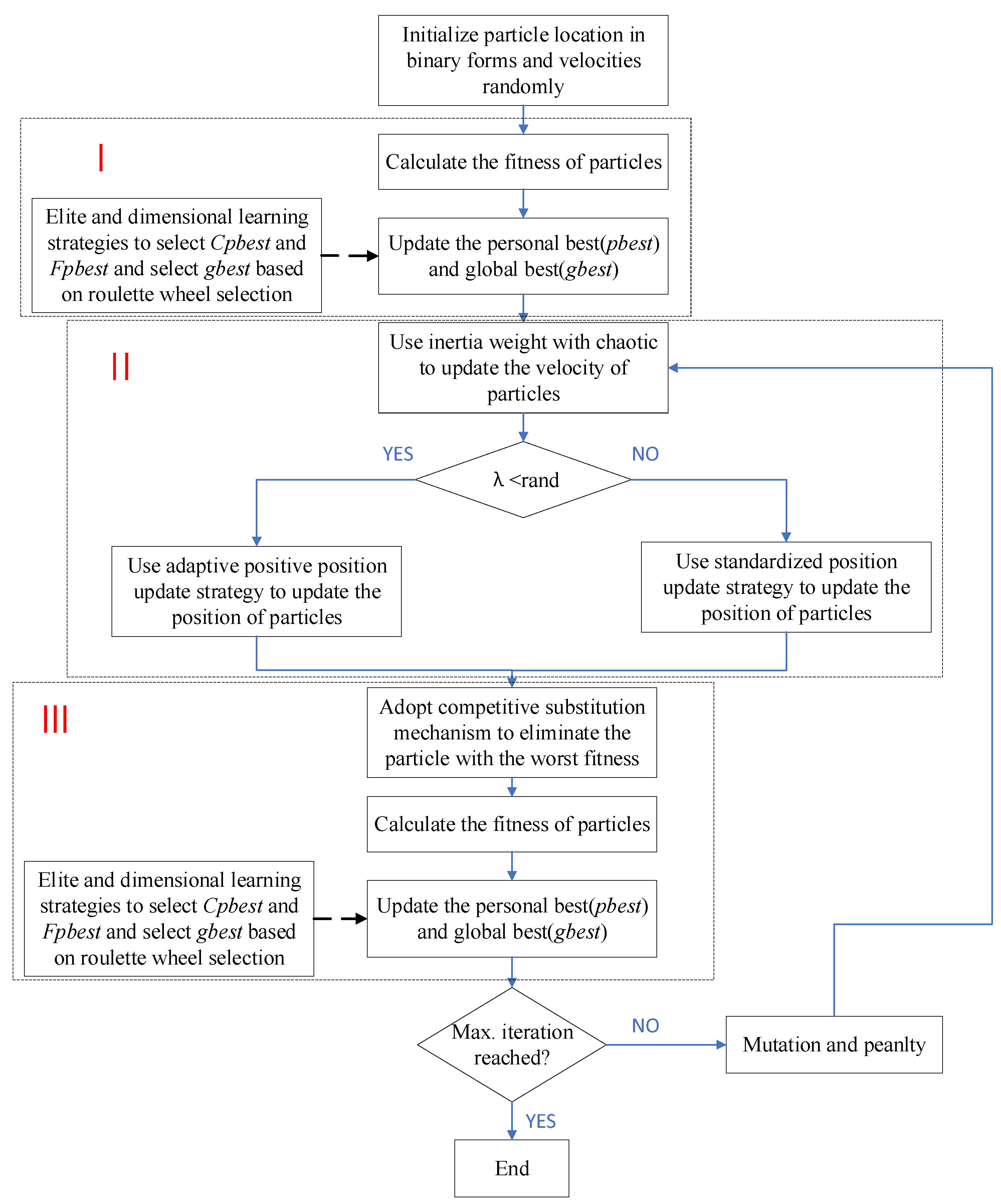
(a) The procedure for renewing the updating method of the global best particle gbest is as follows: the non-dominated particles in the first iteration are stored in the external archive, and then domination comparison between the non-dominated particles in each iteration and the external archive is performed in each iteration. The quantity and occurrence frequency of non-dominated particles in the external archive are computed, and then the global best particle gbest is chosen from among these non-dominated particles by using a roulette wheel based on their occurrence frequency. (b) In the meantime, because the proposed model’s two objectives optimize in the opposing direction, causing inconvenience during the domination decision process, we handle fitness function in the forms of f = [f1,10–f2]. Moreover, the objectives are optimized in the minimal direction, then when the particles do not meet the model’s restrictions we apply the penalty mechanism to those particles, with the associated objectives receiving an additional extreme big value to reduce the calculation workload. (c) In addition, the iteration process takes advantage of the mutation mechanism. At the end of each iteration, each dominated particle will have a probability of acquiring the mutation. The other improvement measures are carried out in the same way as ASPSO. The main flowchart of modified ASPSO in this paper is listed in Figure 6.
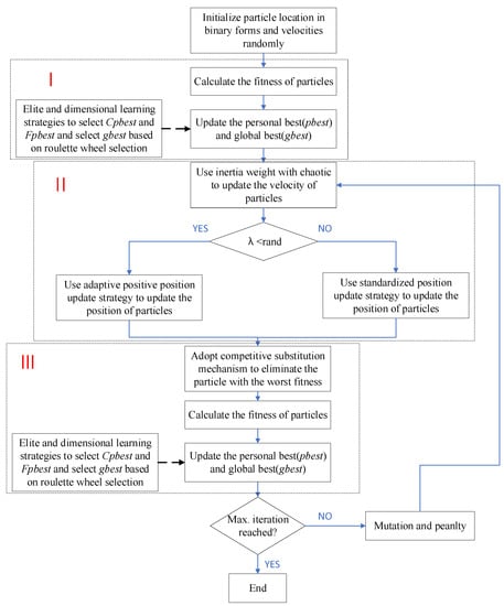
Figure 6.
Flow chart of modified ASPSO.
5. Experimental Results
5.1. Numerical Analysis
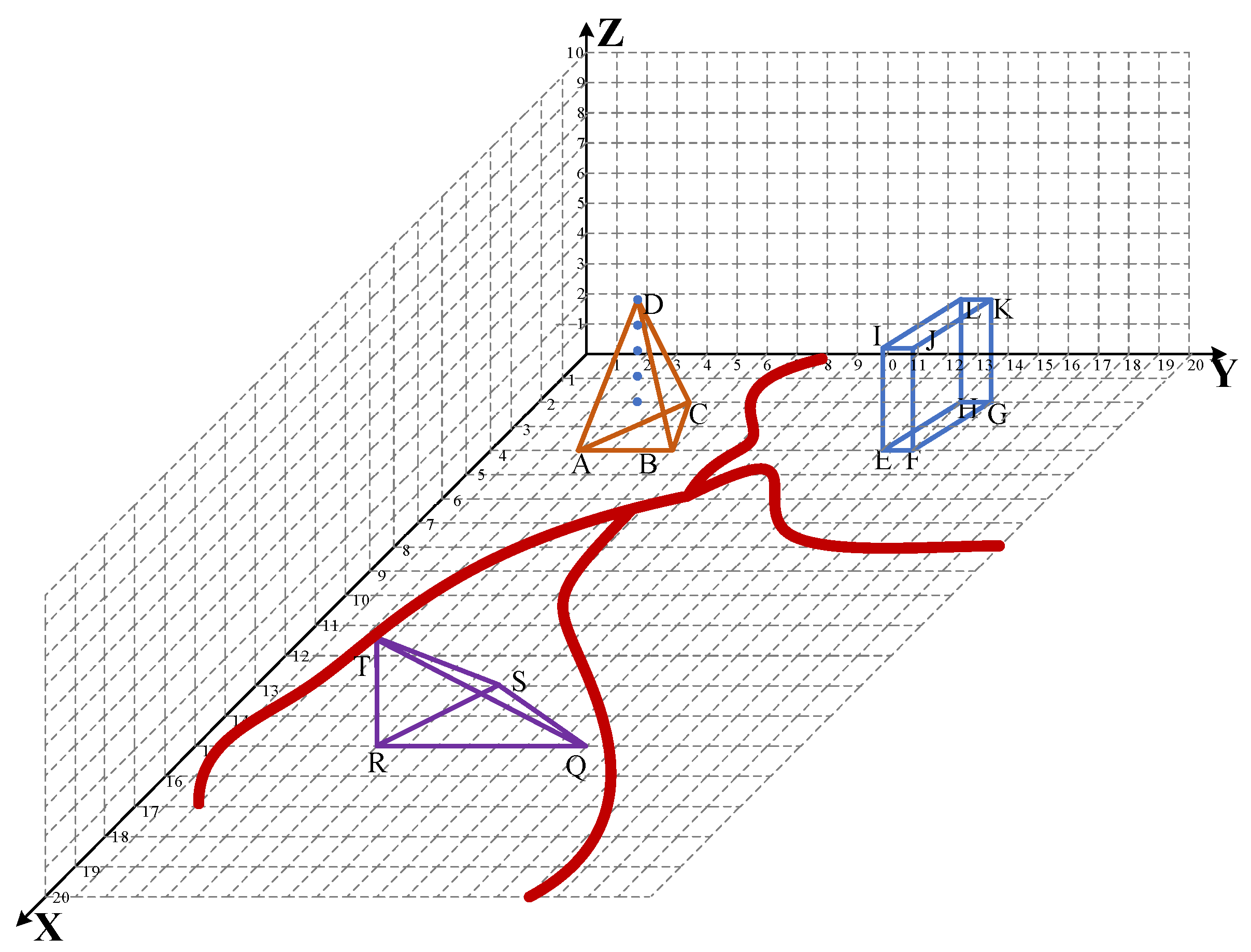
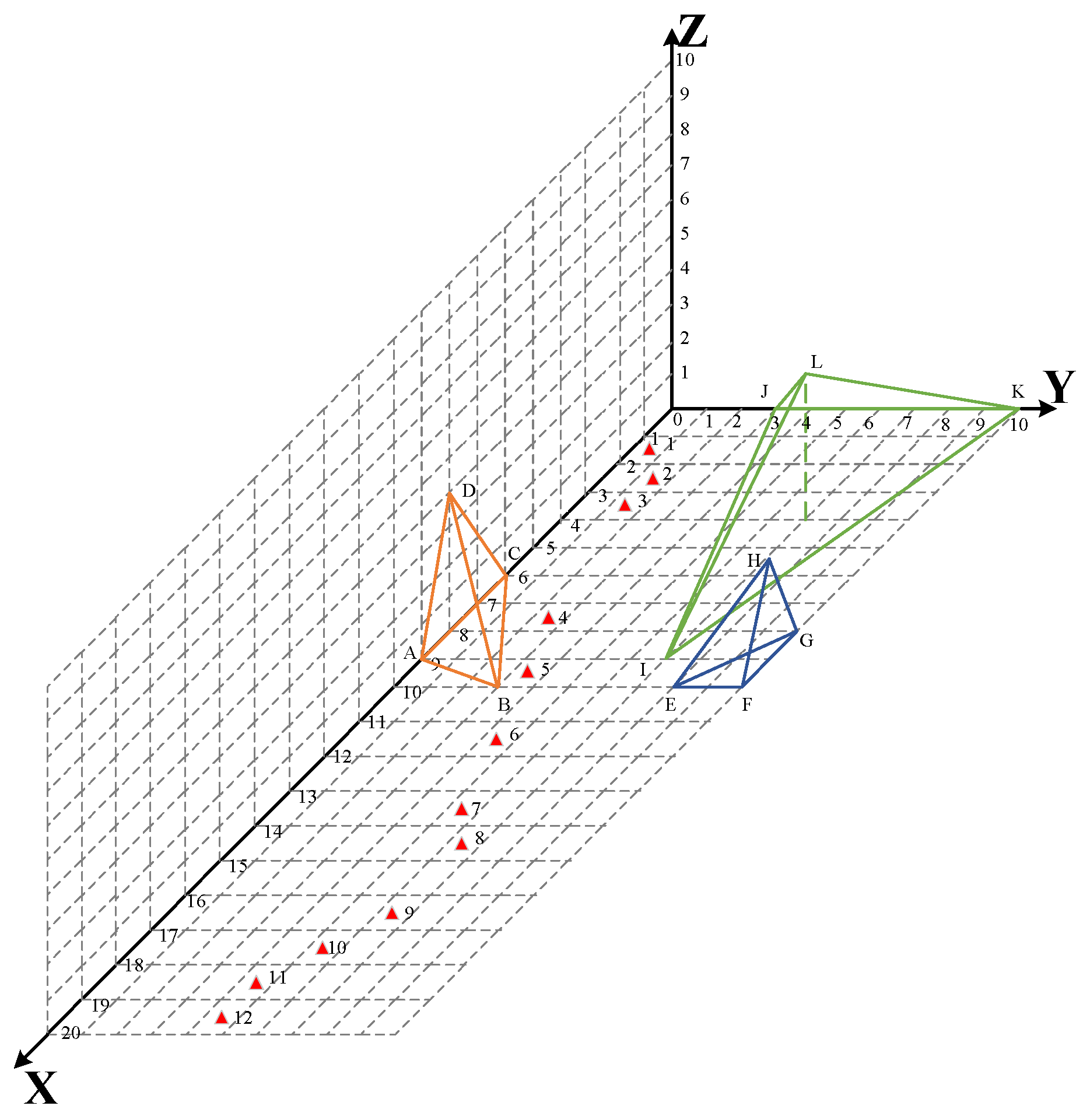
A numerical example is defined that is derived from a real-world VTS radar station location optimization project. The sketch of the VTS radar station environment is depicted in Figure 7. The corresponding parameters are set as follows.
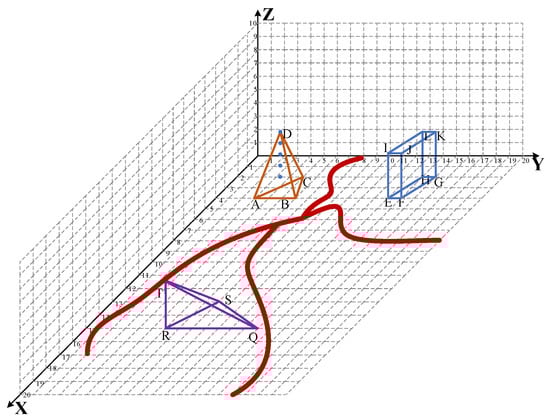
Figure 7.
Sketch of VTS radar station environment.
The entire environment. The range of space of radar station environment varies from 0 to 20 in three dimensions. There are three obstacles in the environment, T-RSQ, D-ABC, and IJKL-EFGH, respectively, the first two obstacles are imitations of the real-world mountains, the third obstacle is an imitation of the real-world forest. The coordinates, elevation, and penetration rate are shown in Table 1. In the surroundings, a river is depicted as a red line in the surrounding area.

Table 1.
Relevant information of obstacles.
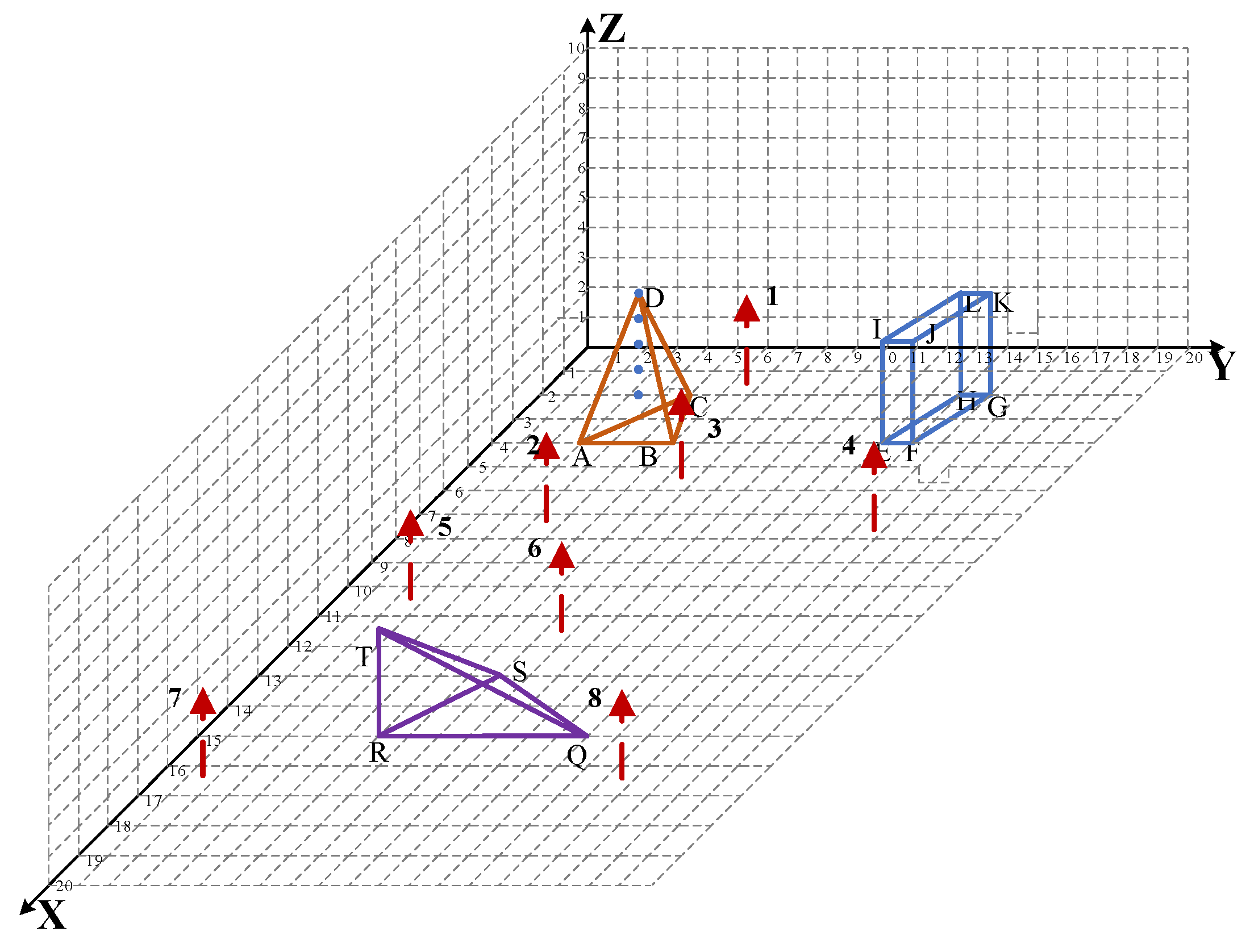
The water area. According to the relevant data of this river provided by local maritime authorities, we segmented the river into eight parts in Figure 8, labeled one to eight in Figure 8. The specific coordinates and area of water area are shown in Table 2.

Figure 8.
Sketch of VTS radar station environment.
Table 2.
Relevant information of water area.
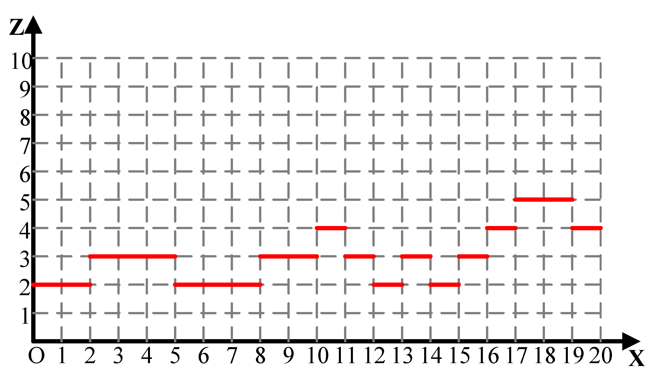
The potential VTS radar station candidate points. All integer points in the three-dimensional space depicted in Figure 7 are possible candidate points for the VTS radar station, the space is produced by the fact that X, Y, and Z all fall within the interval [0, 20]. All candidate points have their corresponding elevations. To facilitate calculation, the elevation of the candidate points is supposed as shown in Figure 9. Meanwhile, the height of the radar station to be built is 1.

Figure 9.
Elevation of candidate points.
The radar coefficients. There are three types of radar available to be configured on the radar station. The specific coefficients for each type of radar are listed in Table 3. It is noted that their maximum coverage radius and configuration cost are both different. As described in Section 3.2, the logarithmic attenuation function adopted in this paper is shown in Equation (16).
Table 3.
Coefficients of radar to be configured.
The following parameters are used in the algorithms: iteration = 100, popsize = 100, poplength = 21 × 21 = 441, the upper limit of non-dominated particles in the external archive is 50, wmax = 0.9, wmin = 0.4, the additional extreme large value is p = 106, and the mutation rate μ is equal to 0.4. Due to the model’s construction being based on maximum coverage and set coverage, it is critical to determine the initial number of VTS radar stations to be built. After multiple attempts in running the algorithm, only when the initial number is greater or equal to 4 can the constraints in the model be fulfilled, in addition, the initial number should be less than 8, which is the number of water areas, otherwise, it is meaningless to carry on this optimization. Therefore, we assume that the number of VTS radar stations to be built is in the interval [4, 7] and obtain the final location program according to the final optimal from the external archive.
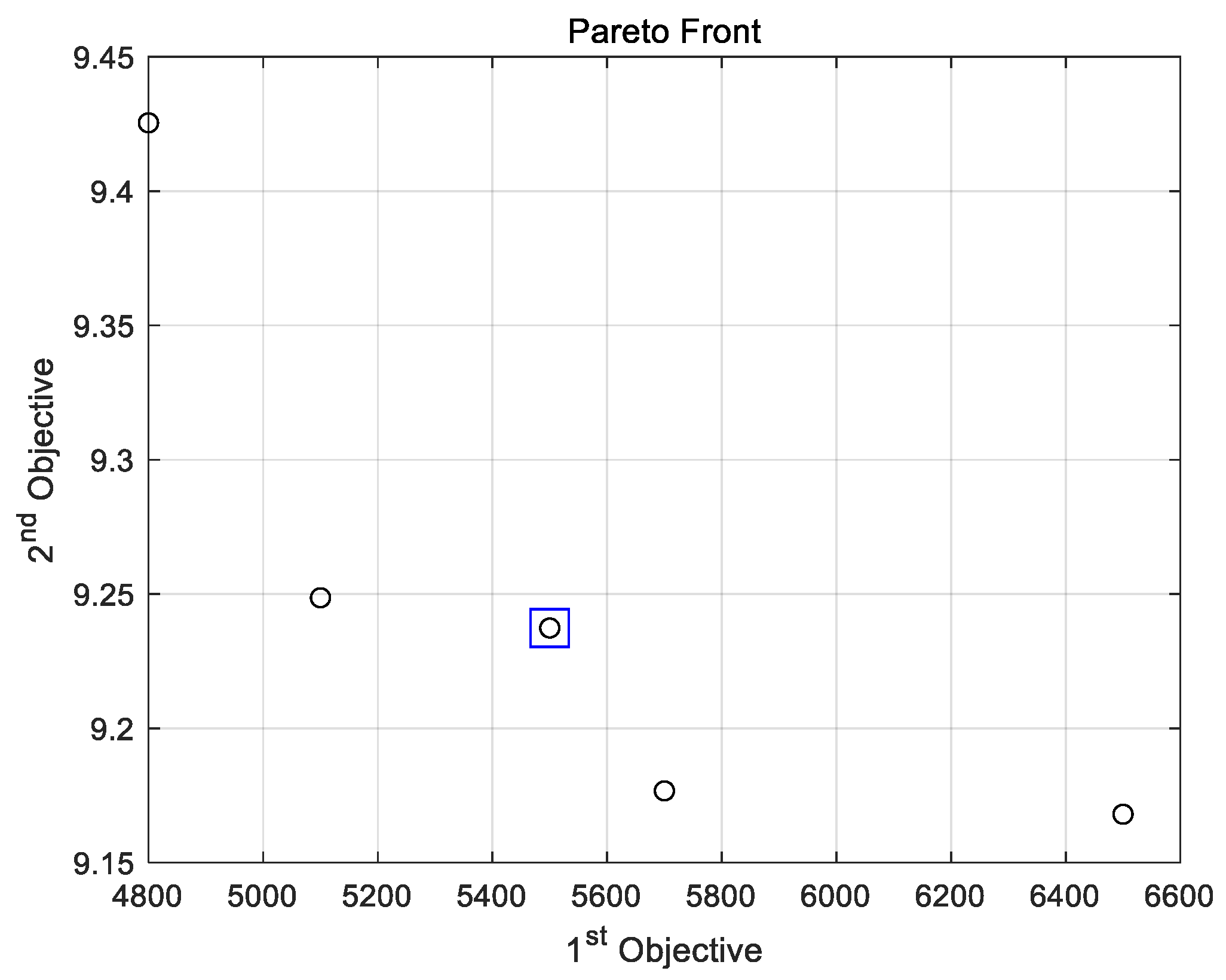
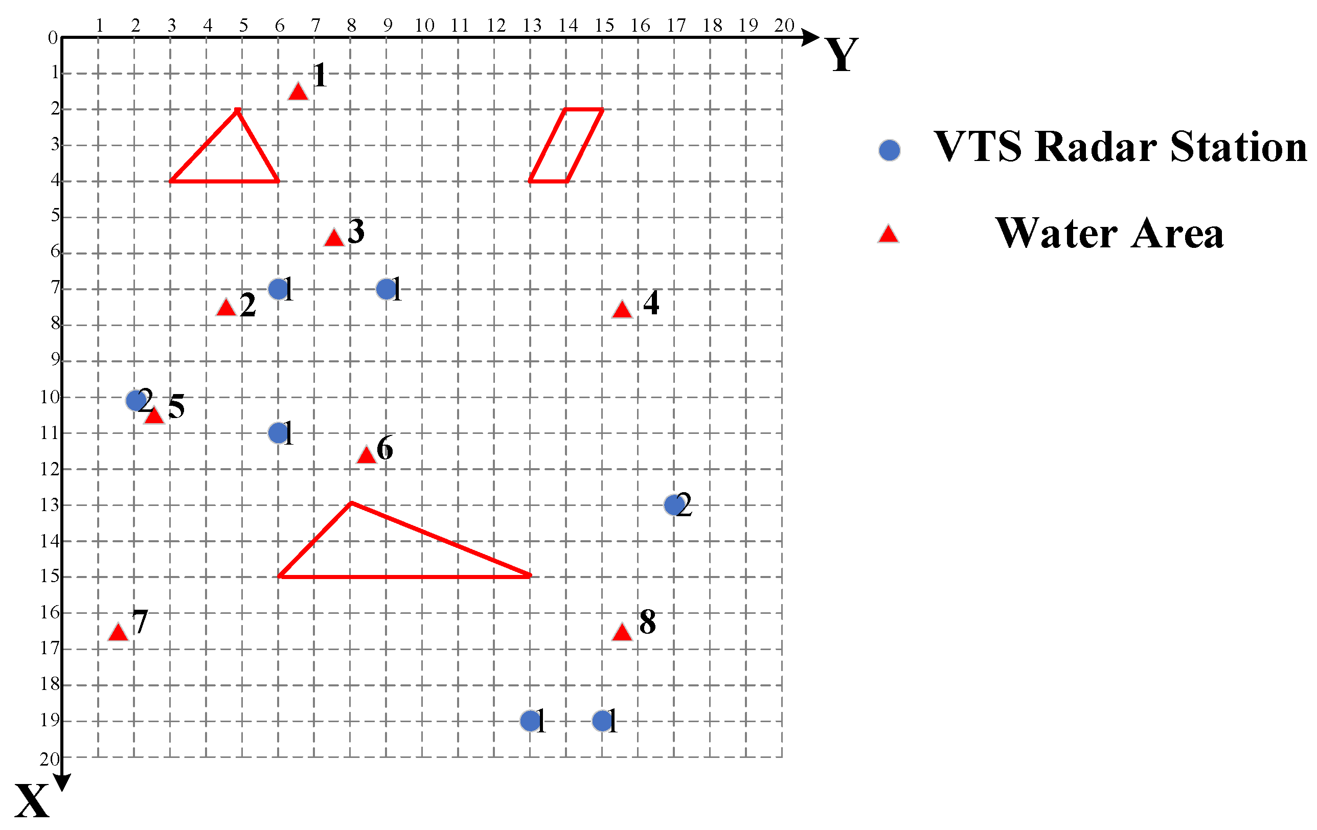
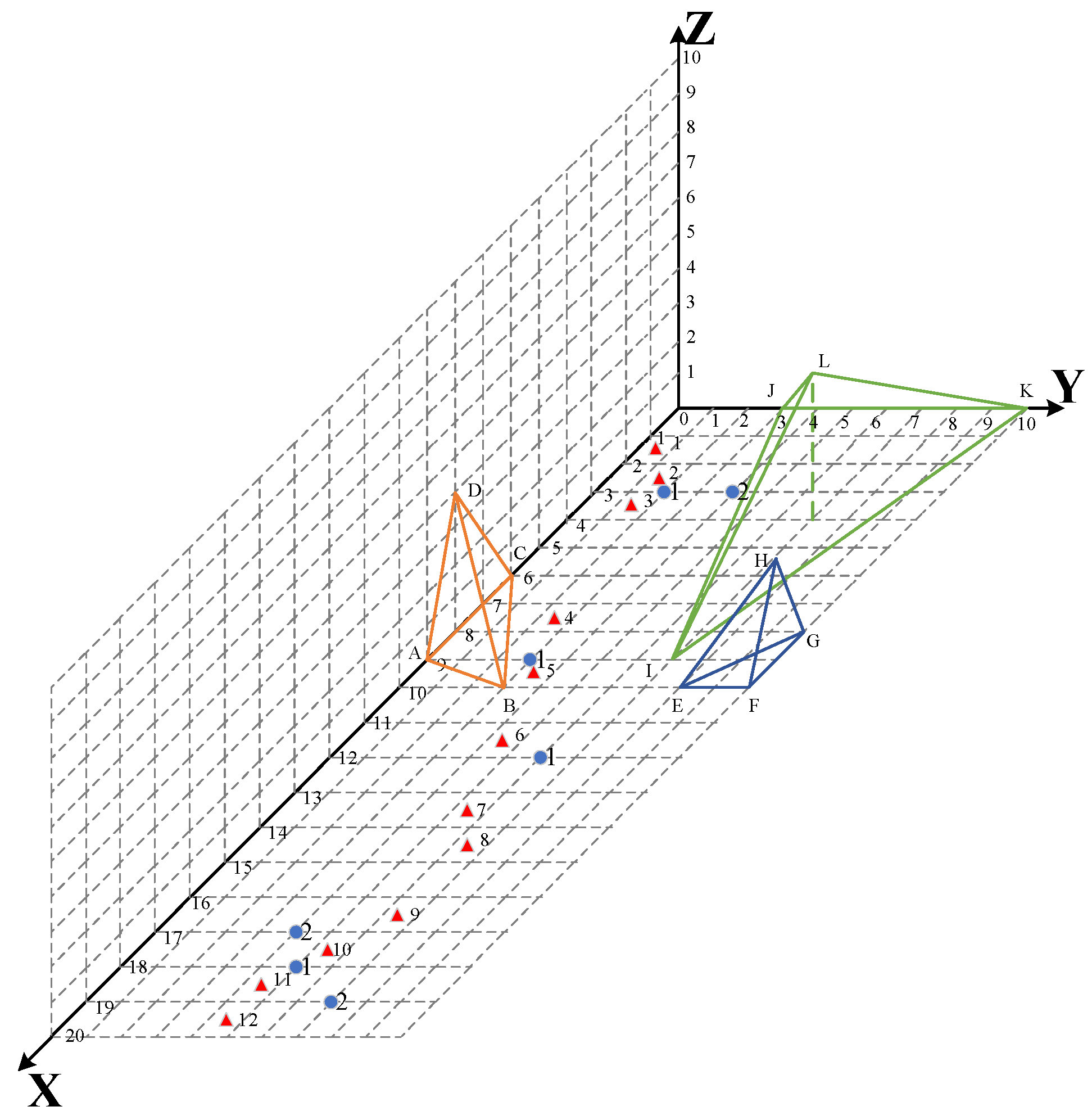
To increase the algorithm’s rationality and accuracy, it was run five times based on the providing parameters. After determining the domination relationship between these non-dominated particles, a Pareto front, and many several non-dominated solutions were formed, as illustrated in Figure 10. However, the final optimal solution cannot still be obtained. As a result, the following approach of determining the ultimate optimal solution from the Pareto front is set as follows. When the algorithm is iterated in the process, the occurrence frequency of each non-dominated particle in the external archive is counted, and then the roulette wheel selection is used between the non-dominated particles in the final Pareto front based on the occurrence frequency, and we can obtain the optimal solution. After the roulette wheel selection process, the particle marked with a square in Figure 10 is the best answer in this paper. According to the optimal solution, when fulfilling the constraints about the multiple covering, 7 candidate points are selected to build the VTS radar station. The total construction cost was 5500 and the coverage rate of the entire water area was 76.26%. Moreover, the corresponding coordinates and configured radar type are shown in Figure 11. To have a good display of the result, Figure 11 is shown in two-dimensional space. Moreover, it was observed that the final solution can cover all water areas in required times and the radar type 1 was preferred to be configured with the candidate points to build increasing.
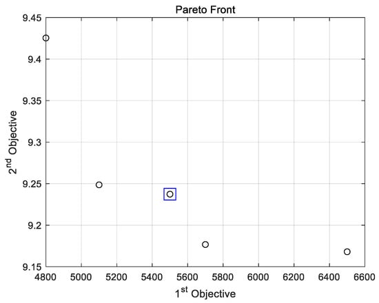
Figure 10.
Pareto front.
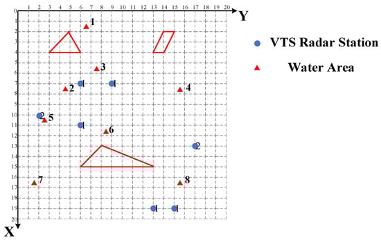
Figure 11.
Distribution map of VTS radar station to be built.
5.2. Case Study
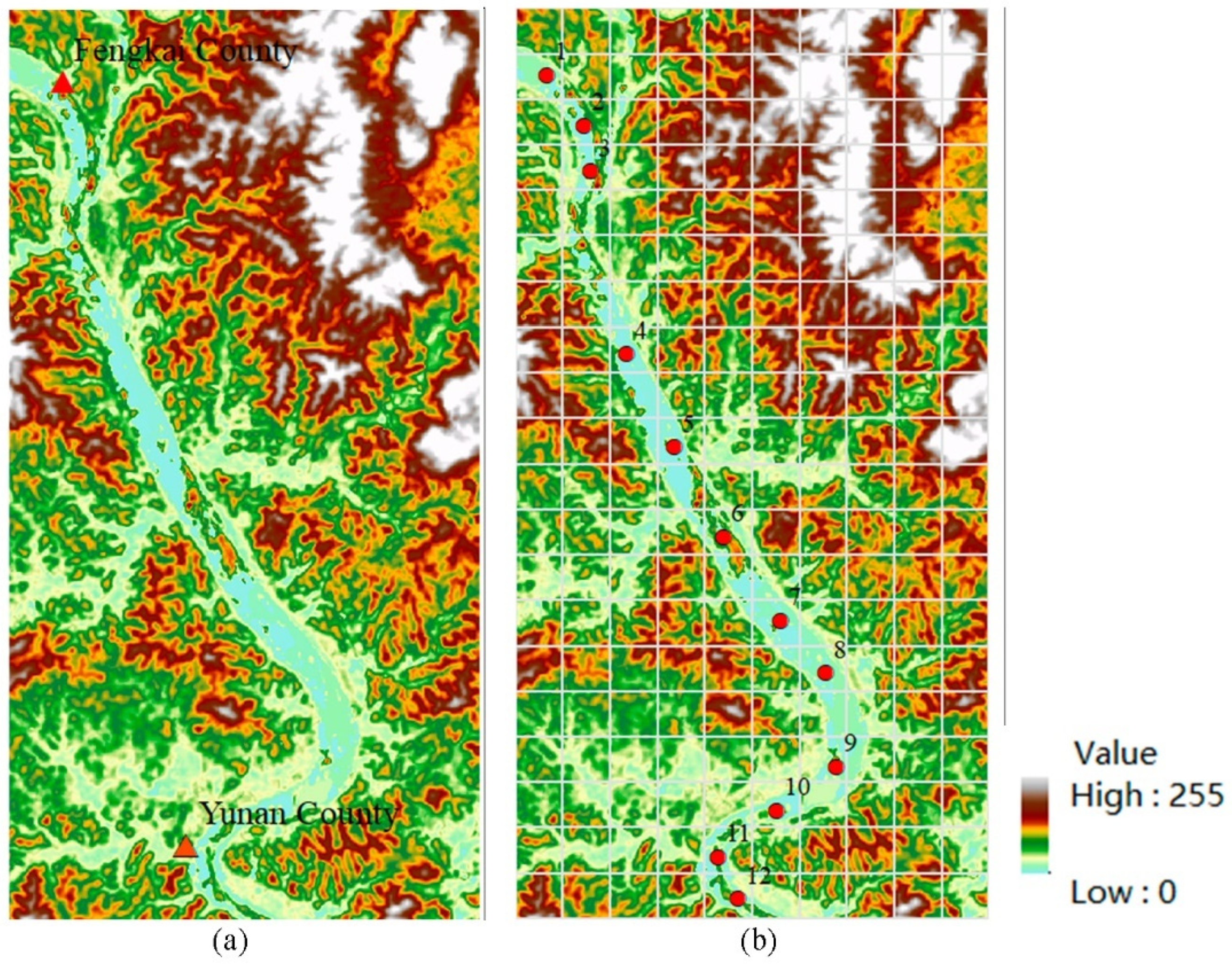
The West River in Zhaoqing, China, between Fengkai and Yunan Counties is used to demonstrate the effectiveness of the suggested model in this research. Figure 12a depicts the environmental digital elevation model image of this water area. As illustrated, this water area is winding and has relatively low elevations. To acquire the coordinates for the water area and radar station candidates, the fishnet function in ArcGIS software was used, and the image was divided into 20 and 10 equal segments along the horizontal and vertical axes, respectively, as illustrated in Figure 12b. Based on the division result, a coordinate system was formed and the water area was divided into 12 parts, as indicated by the sorted red circle in Figure 12b. In Figure 12b, the image’s upper-most and leftmost sides were taken to be the coordinate system’s y and x axes, and thus the x- and y-axis value variation intervals were [0, 20] and [0, 10]. In Figure 12b, the red and white areas represent the environmental obstacles. As a result, the water environment can be simplified to the three-dimensional environment map depicted in Figure 13. The coordinates of the obstacles and the coordinates of the water area are displayed in Table 4 and Table 5. The radar station candidate points are any integer coordinates in Figure 13, the attenuation function is shown in Equation (16), the number of VTS radar stations to be built is in the interval [4, 11] and the remaining parameters are kept constant, after calculating the final Pareto front is shown in Figure 14. After the roulette wheel selection process, the particle marked with a square in Figure 14 is the best answer in this paper. According to the optimal solution, when fulfilling the constraints about the multiple covering, 7 candidate points are selected to build the VTS radar station. The total construction cost is 5900 and the coverage rate of the entire water area is 85%. Moreover, the corresponding coordinates and configured radar type are shown in Figure 15.
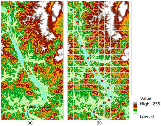
Figure 12.
Environmental digital elevation model image.
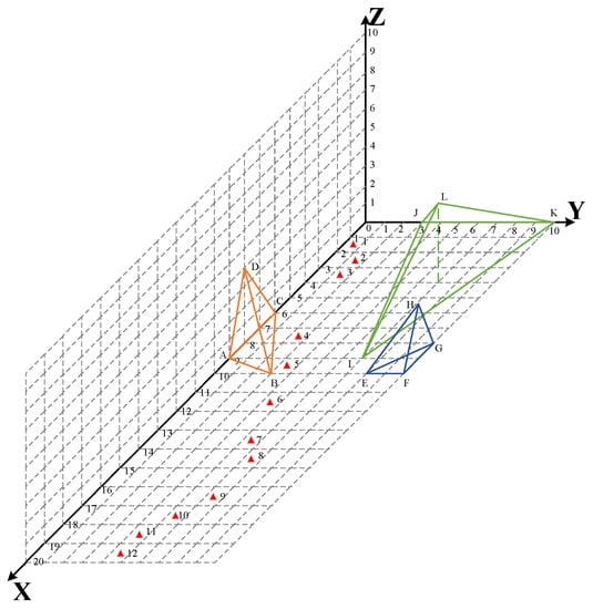
Figure 13.
Environment about West River in three-dimensional space.
Table 4.
Relevant information of obstacles.
Table 5.
Relevant information of water area.
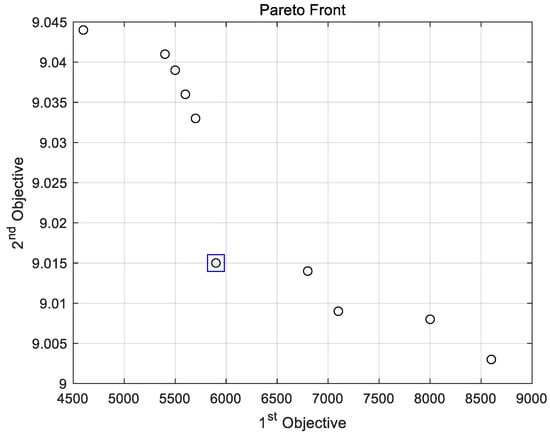
Figure 14.
Pareto front.
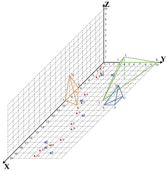
Figure 15.
Distribution map of VTS radar station to be built.
6. Conclusions
This paper investigates the location optimization problem of VTS radar stations in the presence of environmental obstacles and radar attenuation. At present, the majority of research relevant to VTS systems focuses on the VTS systems and VTS operators, and there is a shortage of studies on VTS radar station’s location optimization. Considering the VTS radar station location optimization problem is a facility location problem and the actual environment where VTS radar stations are chosen to build is a three-dimensional space, this paper proposes innovative judgment and evaluation methods about radar attenuation and environmental occlusion and constructs a bi-objective mathematical model based on coverage model. In terms of electromagnetic wave attenuation, the attenuation function based on path loss function in the Okumura–Hata propagation model is introduced to evaluate the effect of attenuation. Moreover, the obstacles such as mountains and forests will generate occlusion during the monitoring process of VTS radar to judge whether the occlusion generates or not the method about environmental occlusion judgment is proposed. After that, a modified adaptive strategy particle swarm optimization algorithm is designed to solve it. Finally, a numerical example is used to verify the effectiveness of the proposed model.
In comparison to the traditional facility location problem in two-dimensional space, the location problem in three-dimensional space in this paper is very similar to the problems encountered in the real world. Consequently, the optimal results in three-dimensional space will be more accurate and scientific. Meanwhile, while taking environmental obstacles and radar attenuation into consideration, the methods and models can provide references when maritime authorities make decisions about the locations of VTS radar stations to improve the economy and effectiveness of the whole system.
In future research, further improvements can be made in terms of algorithms and relevant factors in the construction process, and the comparison of exact solutions and heuristic solutions.
Author Contributions
Conceptualization, Chuan Huang and Jing Lu; methodology, Chuan Huang; software, Jing Lu and Li-Qian Sun; validation, Chuan Huang; formal analysis, Jing Lu; investigation, Li-Qian Sun; resources, Jing Lu, data curation, Jing Lu; writing—original draft preparation, Chuan Huang; writing—review and editing, Jing Lu; visualization, Jing Lu; supervision, Li-Qian Sun; project administration, Jing Lu; funding acquisition, Jing Lu. All authors have read and agreed to the published version of the manuscript.
Funding
This research is supported by the National Natural Science Foundation of China (71974023), the Fundamental Research Funds for the Central Universities (3132019302, 3132021347) and the National Social Science Fund of China (19VHQ012).
Informed Consent Statement
Not applicable.
Data Availability Statement
The data presented in this study are available on request from the corresponding author.
Acknowledgments
This research is supported by the National Natural Science Foundation of China (71974023), the Fundamental Research Funds for the Central Universities (3132019302, 3132021347), and the National Social Science Fund of China (19VHQ012). Any opinions, findings and conclusions, or recommendations expressed in this paper are those of the authors and do not necessarily reflect the views of the sponsors.
Conflicts of Interest
The authors declare no conflict of interest.
Notations
| Set and Matrix | |
| Set of water area | |
| Set of VTS radar station candidate points | |
| Set of VTS radar type | |
| Set of obstacles | |
| Euclidean distance matrix between water areas and candidate points in three-dimensional space | |
| Coverage rate matrix between water areas and candidate points | |
| Parameters | |
| Number of times of water area to be covered | |
| Threshold of number of times of water area | |
| The area coverage rate of water area | |
| Geography area of water area | |
| Total geographical area of the water area | |
| Fixed construction cost of radar station candidate | |
| Configuration cost of radar type | |
| Monitoring probability of radar station candidate when radar type is configured | |
| Minimum effective radius of radar | |
| Maximum effective radius of radar | |
| Attenuation function | |
| Euclidean distance between water area and candidate point | |
| Coverage rate between water area and candidate point | |
| Penetration rate of obstacle | |
| Decision variables | |
| Binary variable, equals 1 if a radar station is constructed at a chosen radar station candidate point and equals 0 otherwise. | |
| Binary variable, equals 1 if a radar station is constructed at a chosen radar station candidate point and the radar type is chosen to be configured meanwhile and equals 0 otherwise. | |
References
- National Bureau of Statistics of the People’s Republic of China. China. 2020. Available online: http://www.stats.gov.cn/ (accessed on 3 March 2022).
- Ministry of Transport of the People’s Republic of China. China. 2020. Available online: http://www.mot.gov.cn (accessed on 3 March 2022).
- Rudan, I.; Francic, V.; Valcic, M.; Sumner, M. Early detection of Vessel collision situations in a vessel traffic services area. Transport 2020, 35, 121–132. [Google Scholar] [CrossRef] [Green Version]
- Gan, L.X.; Yu, F.F.; Zheng, Y.Z.; Zhou, C.-H.; Gao, J.-J.; Cheng, X.-D. Research on modeling and simulation in overshadowing influence of coastal building on vessel traffic service radar. Adv. Mech. Eng. 2018, 10. [Google Scholar] [CrossRef]
- Lee, G.; Kim, S.Y.; Lee, M.K. Economic evaluation of vessel traffic service (VTS): A contingent valuation study. Mar. Policy 2015, 61, 149–154. [Google Scholar] [CrossRef]
- Kao, S.; Lee, K.; Chang, K.; Ko, M.-D. A Fuzzy Logic Method for Collision Avoidance in Vessel Traffic Service. J. Navig. 2007, 60, 17–31. [Google Scholar] [CrossRef]
- Su, C.M.; Chang, K.Y.; Cheng, C.Y. Fuzzy decision on optimal collision avoidance measures for ships in vessel traffic service. J. Mar. Sci. Technol. 2012, 20, 38–48. [Google Scholar] [CrossRef]
- Tsou, M.C. Discovering Knowledge from AIS Database for Application in VTS. J. Navig. 2010, 63, 449–469. [Google Scholar] [CrossRef]
- Tsou, M.C. Online analysis process on Automatic Identification System data warehouse for application in vessel traffic service. Proc. Inst. Mech. Eng. Part M J. Eng. Marit. Environ. 2016, 230, 199–215. [Google Scholar] [CrossRef]
- Relling, T.; Luetzhoeft, M.; Hildre, H.P.; Ostnes, R. How vessel traffic service operators cope with complexity–only human performance absorbs human performance. Theor. Issues Ergon. Sci. 2020, 21, 418–441. [Google Scholar] [CrossRef]
- Chen, H.C.; Lu, H.A.; Lee, H.H. An assessment of job performance of vessel traffic service operations using an analytic hierarchy process and a grey interval measure. J. Mar. Sci. Technol. 2013, 21, 522–531. [Google Scholar]
- Praetorius, G.; Hollnagel, E.; Dahlman, J. Modelling Vessel Traffic Service to understand resilience in everyday operations. Re-Liabil. Eng. Syst. Saf. 2015, 141, 10–21. [Google Scholar] [CrossRef]
- Jia, S.; Wu, L.X.; Meng, Q. Joint Scheduling of Vessel Traffic and Pilots in Seaport Waters. Transp. Sci. 2020, 54, 1495–1515. [Google Scholar] [CrossRef]
- Relling, T.; Lutzhoft, M.L.; Ostnes, R.; Hildre, H.P. The contribution of Vessel Traffic Services to safe coexistence between automated and conventional vessels. Marit. Policy Manag. 2021; early access. [Google Scholar]
- Brodje, A.; Lundh, M.; Jenvald, J.; Dahlman, J. Exploring non-technical miscommunication in vessel traffic service operation. Cogn. Technol. Work 2013, 15, 347–357. [Google Scholar] [CrossRef]
- Mansson, J.; Lutzhoft, M.; Brooks, B. Joint Activity in the Maritime Traffic System: Perceptions of Ship Masters, Maritime Pilots, Tug Masters, and Vessel Traffic Service Operators. J. Navig. 2017, 70, 547–560. [Google Scholar] [CrossRef]
- Costa, N.A.; MacKinnon, S.N. Non-technical communication factors at the Vessel Traffic Services. Cogn. Technol. Work 2018, 20, 63–72. [Google Scholar] [CrossRef] [Green Version]
- Li, F.; Chen, C.; Xu, G.; Chang, D.; Khoo, L.P. Causal Factors and Symptoms of Task-Related Human Fatigue in Vessel Traffic Service: A Task-Driven Approach. J. Navig. 2020, 73, 1340–1357. [Google Scholar] [CrossRef]
- Malagoli, A.; Corradini, M.; Corradini, P.; Shuett, T.; Fonda, S. Towards a method for the objective assessment of cognitive workload: A pilot study in vessel traffic service (VTS) of maritime domain. In Proceedings of the 2017 IEEE 3rd International Forum on Research and Technologies for Society and Industry (RTSI), Modena, Italy, 11–13 September 2017; pp. 1–6. [Google Scholar]
- Xu, G.Y.; Chen, C.H.; Li, F.; Qiu, X. AIS data analytics for adaptive rotating shift in vessel traffic service. Ind. Manag. Data Syst. 2020, 120, 749–767. [Google Scholar] [CrossRef]
- Lei, Z.; Tao, M.; Kun, H.; Wei, Q. Advances in full control of electromagnetic waves with meta-surfaces. Adv. Opt. Mate-Rials 2016, 4, 818–833. [Google Scholar]
- Singh, Y. Comparison of Okumura, Hata and COST-231 Models on the Basis of Path Loss and Signal Strength. Int. J. Comput. Appl. 2012, 59, 37–45. [Google Scholar] [CrossRef]
- Muhammad, F.; Amr, E.K.; Ahmed, S. Empirical Correction of the Okumura-Hata Model for the 900 MHz band in Egypt. In Proceedings of the IEEE 2013 Third International Conference on Communications and Information Technology, Beirut, Lebanon, 19–21 June 2013; pp. 386–395. [Google Scholar]
- Tasmeeh, A.; Fariha, J.; Mannan, P. Inspection of Picocell’s Performance using Different Models in Different Regions. In Proceedings of the IEEE 2020 5th International Conference on Computer and Communication Systems, Shanghai, China, 22–24 February 2020. [Google Scholar]
- Mahmoud, A.; Zia, N.; Hassan, A. Applicability of Okumura-Hata Model for Wireless Communication Systems in Oman. In Proceedings of the IEEE International IOT, Electronics and Mechatronics Conference, Vancouver, BC, Canada, 9–12 September 2020. [Google Scholar]
- Vera, D.; Ruslan, A. Ordinary Least Squares in COST 231 Hata key parameters optimization base on experimental data. In Proceedings of the IEEE 2017 International Multi-Conference on Engineering, Computer and Information Sciences, Hong Kong, 15–17 March 2017. [Google Scholar]
- Keun, Y.; Won, J.; Ho, K. Intelligent Ray Tracing for the Propagation Prediction. In Proceedings of the 2012 IEEE Antennas and Propagation Society International Symposium, Chicago, IL, USA, 8–14 July 2012. [Google Scholar]
- Zheng, Y.; Magdy, I. Ray Tracing for Radio Propagation Modeling: Principles and Applications. IEEE Access 2015, 3, 1089–1100. [Google Scholar]
- Wanderley, P.H.; Terada, M.A. Assessment of the applicability of the Ikegami propagation model in modern wireless communication scenarios. J. Electromagn. Waves Appl. 2012, 26, 1483–1491. [Google Scholar] [CrossRef]
- Har, D.; Watson, A.M.; Chadney, A.G. Comment on diffraction loss of rooftop-to-street in COST 231-Walfisch-Ikegami model. IEEE Trans. Veh. Technol. 1999, 48, 1451–1458. [Google Scholar] [CrossRef]
- Karatas, M. A multi-objective facility location problem in the presence of variable gradual coverage performance and coopertive cover. Eur. J. Oper. Res. 2017, 262, 1040–1051. [Google Scholar] [CrossRef]
- Wang, B.C.; Qian, Q.Y.; Gao, J.J.; Tan, Z.Y.; Zhou, Y. The optimization of warehouse location and resources distribution for emergency rescue under uncertainty. Adv. Eng. Inform. 2021, 48, 101278. [Google Scholar] [CrossRef]
- Du, B.; Zhou, H.; Leus, R. A two-stage robust model for a reliable p-center facility location problem. Appl. Math. Model. 2010, 77, 99–114. [Google Scholar] [CrossRef]
- Tedeschi, D.; Andretta, M. New exact algorithms for planar maximum covering location by ellipses problems. Eur. J. Oper. Res. 2021, 291, 114–127. [Google Scholar] [CrossRef]
- Baray, J.; Cliquet, G. Optimizing locations through a maximum covering/p-median hierarchical model: Maternity hospitals in France. J. Bus. Res. 2013, 66, 127–132. [Google Scholar] [CrossRef]
- Vieira, B.S.; Ferrari, T.; Ribeiro, G.M.; Bahiense, L.; Filho, R.D.O.; Abramides, C.A.; Júnior, N.F.R.C. A progressive hybrid set covering based algorithm for the traffic counting location problem. Expert Syst. Appl. 2020, 160, 113641. [Google Scholar] [CrossRef]
- Sinnl, M. Exact and heuristic algorithms for the maximum weighted submatrix coverage problem. Eur. J. Oper. Res. 2021; early access. [Google Scholar]
- Li, J.L.; Liu, Z.B.; Wang, X.F. Public charging station location determination for electric ride-hailing vehicles based on an im-proved genetic algorithm. Sustain. Cities Soc. 2021, 74, 103181. [Google Scholar] [CrossRef]
- Marinakis, Y. An improved particle swarm optimization algorithm for the capacitated location routing problem and for the location routing problem with stochastic demands. Appl. Soft Comput. 2015, 37, 680–701. [Google Scholar] [CrossRef]
- Rohaninejad, M.; Sahraeian, R.; Tavakkoli-Moghaddam, R. An accelerated Benders decomposition algorithm for reliable facility location problems in multi-echelon networks. Comput. Ind. Eng. 2018, 124, 523–534. [Google Scholar] [CrossRef]
- Vaze, R.; Deshmukh, N.; Kumar, R.; Saxena, A. Development and application of Quantum Entanglement inspired Particle Swarm Optimization. Knowl.-Based Syst. 2021, 219, 106859. [Google Scholar] [CrossRef]
- Squires, M.; Tao, X.; Elangovan, S.; Gururajan, R.; Saxena, A. A novel genetic algorithm based system for the scheduling of medical treatments. Expert Syst. Appl. 2022, 195, 116464. [Google Scholar] [CrossRef]
- Khan, S.; Grudniewski, P.; Muhammad, Y.; Sobey, A. The benefits of co-evolutionary Genetic Algorithms in voyage optimisa-tion. Ocean. Eng. 2022, 245, 110261. [Google Scholar] [CrossRef]
- Zeng, Z.; Zhang, M.; Hong, Z.; Zhang, H.; Zhu, H. Enhancing differential evolution with a target vector replacement strategy. Comput. Stand. Interfaces 2022, 82, 103631. [Google Scholar] [CrossRef]
- Morais, M.; Ribeiro, M.; Silva, R.; Mariani, V.; Coelho, L. Discrete differential evolution metaheuristics for permutation flow shop scheduling problems. Comput. Ind. Eng. 2022, 166, 107956. [Google Scholar] [CrossRef]
- Jaafari, A.; Panahi, M.; Gholami, D.; Rahmati, O.; Shahabi, H.; Shirzadi, A.; Lee, S.; Bui, D.T.; Pradhan, B. Swarm intelligence optimization of the group method of data handling using the cuckoo search and whale optimization algorithms to model and predict landslides. Appl. Soft Comput. 2022, 116, 108254. [Google Scholar] [CrossRef]
- Peng, J.; Li, Y.; Kang, H.; Shen, Y.; Sun, X.; Chen, Q. Impact of population topology on particle swarm optimization and its variants: An in-formation propagation perspective. Swarm Evol. Comput. 2022, 69, 100990. [Google Scholar] [CrossRef]
- Cui, Y.; Meng, X.; Qiao, J. A multi-objective particle swarm optimization algorithm based on two-archive mechanism. Appl. Soft Comput. 2022, 119, 108532. [Google Scholar] [CrossRef]
- Singh, S.; Bansal, J. Mutation-driven grey wolf optimizer with modified search mechanism. Expert Syst. Appl. 2022, 194, 116450. [Google Scholar] [CrossRef]
- Adhikary, J.; Acharyya, S. Randomized Balanced Grey Wolf Optimizer (RBGWO) for solving real life optimization prob-lems. Appl. Soft Comput. 2022, 117, 108429. [Google Scholar] [CrossRef]
- Boumedine, N.; Bouroubi, S. Protein folding in 3D lattice HP model using a combining cuckoo search with the Hill-Climbing algorithms. Appl. Soft Comput. 2022, 119, 108564. [Google Scholar] [CrossRef]
- Bajaj, A.O. Sangwan Discrete cuckoo search algorithms for test case prioritization. Appl. Soft Comput. 2021, 110, 107584. [Google Scholar] [CrossRef]
- Kyriakakis, N.; Marinaki, M.; Matsatsinis, N.; Marinakis, Y. Moving peak drone search problem: An online multi-swarm intelli-gence approach for UAV search operations. Swarm Evol. Comput. 2021, 66, 100956. [Google Scholar] [CrossRef]
- Engelbrecht, A.P. Computational Intelligence: An Introduction; John Wiley & Sons: Hoboken, NJ, USA, 2007. [Google Scholar]
- Wang, R.; Hao, K.R.; Chen, L.; Wang, T.; Jiang, C. A novel hybrid particle swarm optimization using adaptive strategy. Inf. Sci. 2021, 579, 231–250. [Google Scholar] [CrossRef]


Publisher’s Note: MDPI stays neutral with regard to jurisdictional claims in published maps and institutional affiliations. |
© 2022 by the authors. Licensee MDPI, Basel, Switzerland. This article is an open access article distributed under the terms and conditions of the Creative Commons Attribution (CC BY) license (https://creativecommons.org/licenses/by/4.0/).