All Burglaries Are Not the Same: Predicting Near-Repeat Burglaries in Cities Using Modus Operandi

Abstract

The evidence that burglaries cluster spatio-temporally is strong. However, research is unclear on whether clustered burglaries (repeats/near-repeats) should be treated as qualitatively different crimes compared to spatio-temporally unrelated burglaries (non-repeats). This study, therefore, investigated if there were differences in modus operandi-signatures (MOs, the habits and methods employed by criminals) between near-repeat and non-repeat burglaries across 10 Swedish cities, as well as whether MO-signatures can aid in predicting if a burglary is classified as a near-repeat or a non-repeat crime. Data consisted of 5744 residential burglaries, with 137 MO features characterizing each case. Descriptive data of repeats/non-repeats is provided together with Wilcoxon tests of MO-differences between crime pairs, while logistic regressions were used to train models to predict if a crime scene was classified as a near-repeat or a non-repeat crime. Near-repeat crimes were rather stylized, showing heterogeneity in MOs across cities, but showing homogeneity within cities at the same time, as there were significant differences between near-repeat and non-repeat burglaries, including subgroups of features, such as differences in mode of entering, target selection, types of goods stolen, as well the traces that were left at the crime scene. Furthermore, using logistic regression models, it was possible to predict near-repeat and non-repeat crimes with a mean F${}_1$-score of $0.8155$ ($0.0866$) based on the MO. Potential policy implications are discussed in terms of how data-driven procedures can facilitate analysis of spatio-temporal phenomena based on the MO-signatures of offenders, as well as how law enforcement agencies can provide differentiated advice and response when there is suspicion that a crime is part of a series as opposed to an isolated event.

1. Introduction

The spatio-temporal signatures for when and where crimes are committed are different dependent on crime categories [1,2]. A number of studies have confirmed empirical regularities for burglaries [3,4,5], suggesting that once a household is burglarized, the risk increases of being burglarized again, not only for the victim (repeat) but also for their neighbours (near-repeat) [3,6,7,8].

Researchers, as well as law enforcement agencies, have identified patterns across different timescales (e.g., hours, days, weeks and years) and spatial levels (e.g., nation, region, community, and neighborhood down to street level). Finding spatio-temporal patterns aids in developing a holistic and differentiated understanding in comparison to analyzing crimes in isolation [9], which may help prediction of future crime locations [10]. However, recent research has also raised questions about the viability of using repeat victimization assumptions in crime prevention. For instance, in a New Zealand based study, at least half of the burglaries (repeats and near repeats) were located outside hotspots [11].

In order to enrich description, as well as potentially to increase the chances of linking the crimes of offenders, spatio-temporal analysis could be complemented with physical evidence, such as DNA or fingerprints. Unfortunately, such evidence is not always available at crime scenes and is more frequently available for certain crime categories than for others [12]. The processing of physical evidence is also very costly and time-consuming. Thus, it is difficult for law enforcement agencies to handle large amounts of physical evidence from high-volume crime categories [13], such as burglaries.

Another, complementary, approach to the spatio-temporal aspect of crime is to focus on “soft evidence” associated with offenders’ modus operandi (MO), i.e., habits, techniques and peculiarities of behaviour when committing an offence, such as using a particular entrance or a specific tool when breaking into a building [2,14]. For instance, such cues may highlight if an offender uses repetitive (consistent) or varying (specific) behaviour in terms of tools or point of access to a house/apartment. This type of evidence may, in turn, depend on characteristics of the environment and, thus, vary between burglaries. Evidence is most often available to collect if adequately designed methods to investigate the crime scene are used. Any collected crime scene data may be interpreted using behavioural and criminal profiling [15,16,17] in a manner that reflects the perpetrator’s cognitions [18], degree of risk-taking and planning [19,20], and thus provide a richer description of an offender’s actions that will further aid in prediction of when and where they will commit crimes again. However, in reality, such analyses are often conducted by means of individual law enforcement officers and are rarely undertaken using systematic data-driven comparisons across cases, cities and regions.

There are examples of studies, however, that jointly analyze MOs or household variables with spatio-temporal aspects (repeat/near-repeat). These exceptions include the study of Bowers and Johnson [21], where the point of entry and method of entry in 3562 cases were analyzed, and in Vandeviver et al. [20], a study where 650 cases were compared to nearby housing characteristics (500,000 residential properties). However, although previous research supports the view that single offenders may be likely to return to the same or nearby burglary scene [5], the rationale for recidivism can be questioned on the basis that MO-signatures may not be a consequence of a single offender. Burglaries are often conducted in small groups where offenders may interact and generate knowledge spillovers (see Glaeser et al. [22]). Committing crimes in groups would therefore blur an individual’s specific MO as the crime depends on aggregated MOs. Thus, the “socialness” of burglaries emphasizes a different view of the utility of MOs in space and time. An aggregated spatio-temporal bound MO-signature would help discriminate repeat from non-repeat crimes, regardless of whether the offender is working alone or in a group.

Thus, an analysis of the temporal and spatial distribution of burglaries, combined with the features that characterize and potentially discriminate these crimes, can provide an enriched description of offender whereabouts. This can have important policy implications in terms of possible proactive procedures for how to avoid crimes, as well as how the police force’s scarce resources should be strategically and efficiently used [23].

More specifically, in this study, we investigated the spatio-temporal distribution (in terms of near-repeat/repeat) of burglaries across 10 Swedish cities, examining whether there were differences in MOs between near-repeat/repeat versus non-repeat burglaries and whether it was possible to estimate the probability that a crime scene was a part of a repeat chain (near-repeat or repeat), based on the features of the crime-scene and the offenders’ MOs. We also investigated how features indicative of near-repeat crimes differed between different cities. The investigation was based on data on residential burglaries in cities in Sweden between 2012 and 2016.

2. Theoretical Background

2.1. Theories of Criminal Behavior

Crime is about an actor(s), the environment, and the interaction between the two [24]. Previously, and from a rational economic perspective, criminal behaviour has been understood to involve a systematic assessment of benefits against the potential risk of punishment if caught [25]. Although it may be difficult to obtain complete information about a potential target, recent research supports the view of burglars’ rational deliberation in target selection [20]. In contrast to the rational choice model of individuals committing crimes, advocates of routine activity theory assume that criminal behaviour is victim orientated, habitual and entails a much less deliberate course of action by the offender [26,27]. Routine activity theory further suggests that offenders’ target selection is shaped by successful criminal activity [28]. Thus, in broad terms, while rational choice theory focuses on the deliberation of an individual perpetrator, routine activity theory focuses on collective and contextual determinants of victimization.

Despite the diverging rationales for committing crime in rational choice and routine activity theory, the two streams of research complement each other in describing the patterns underpinning crime in time and space, highlighting assumptions that underpin repeat and near-repeat patterns. In line with rational choice theory, if a utility assessment renders a calculus of low punishment, this may consequently cause the perpetrator to revisit the crime scene, if risk estimates are kept low in the calculus. Similar accounts have also been put forward in, for instance, optimal foraging theory [21,29], which highlights assessment of immediate return in relation to the risk and effort of seeking new possibilities, and the boost account, which states that return to a crime scene is dependent on previous success [21], such as having a high payoff. Routine activity theory [26] implies that recurring patterns of the victims’ situation flags vulnerability and thus encourages perpetrators to commit a first crime, but also to habitually revisit the crime scene due to its ease of accessibility. Furthermore, research suggests that offenders tend to return to an area if they have previously committed a crime close by, the probability increasing if the crime types are similar, the more recently the previous crime took place, or as the number of previous crimes increases [5,30]. Thus, these theories inform our study as they aid in explaining the rationale for repeat and near repeat crimes, as long as it is assumed that it is the same perpetrator who commits the crimes.

However, repeat and near-repeat crimes are not necessarily conducted by the same individual. Socioeconomic research reveals less severe crimes to be a “social” activity where contagious effects occur [31,32]. These petty crimes (such as car thefts) and moderate crimes (such as burglaries) are particularly susceptible to higher degrees of social interaction among criminals in comparison to more violent crimes, such as rape or murder [22]. Thus, to develop further understanding of patterns of crime, as well as what and offenders may engage in interaction about and when, the relative influence of external factors, such as housing features, and MO-features, such as means of entry, need to be jointly analyzed in space and time. As will be described below, previous studies have relied on limited sets of data, either in terms of features, or the number of cases analyzed. Next, therefore, we review empirical regularities of spatio-temporally distributed crime together with the specific features, such as the MO, characterizing these burglaries.

2.2. Empirical Regularities of Temporal, Spatial and Repetitive Aspects of Crime

As previously described, burglaries tend to cluster in space and time, making it likely households are re-victimized (or nearby households become victims). Early research by [33] showed patterns of repeat victimisation to account for a significant amount of crime in England and Wales. More recent research showed burglaries to be highly concentrated within cities (across several different countries). For instance, in studies by [34,35] in Vancouver and Ottawa, a high percentage of calls to the police service regarding burglaries came from a very small number of addresses. Similar results were shown in [36], a study in Tel-Aviv Jaffa, Israel, raising the possibility of generalization about crime concentration in space.

With respect to the features used to analyze domestic burglaries, the past decade has produced a surge in studies focusing on space and time-related issues. Hot-spot analysis has been a commonly used technique to group cases based on spatial information, with the intention of predicting future crimes [12,37,38,39,40,41,42]. These studies have highlighted that areas that have previously been burgled face the risk of being burgled again [21,33].

Moreover, not only does the location matter, but so do aspects of housing. For instance, in a study from the Netherlands, terraced houses, houses without a garage, houses that had not been fitted with a central heating and/or air-conditioning system, and houses near to burglars’ residences, were more likely to be burglarized [20]. In addition, proximity of Australian households with a high degree of housing homogeneity is associated with a similar level of elevated risk to the temporally related risk of becoming a victim [32]. In another study, which focused on (near) repeats in Belo Horizonte in Brazil, areas with heterogeneous housing, such as fencing of the perimeters, an increase in guards, irregular and self-constructed housing, showed a lower degree of (near) repeats than Western housing [6]. In other words, diversity in physical construction seems to safeguard against perpetrators committing (near) repeat crimes.

With respect to temporal relationships, offended-against households are likely to be struck again [5]. A large study, which compared burglaries from five different nations found that houses within 200 m of a burgled home faced an elevated risk of burglary within the next two weeks [4]. Moreover, the time course of repeats (revictimization within seven days) has also been found to occur at the same time/weekday as the antecedent event [43,44]. The temporal bandwidth that has been used to assess near repeats has typically ranged between 1 and 14 days [6].

The examination of spatio-temporal aspects of domestic burglaries has utilised different levels of analysis. Spatial criminology is enhanced by varying the resolution from the macro, through neighbourhood, to street level analysis. By using spatial point patterns, Ref. [2] found that general crime patterns are similar at several spatial scales, but analysis at finer levels (such as street segments) revealed significant variations within larger units, suggesting that crime was a quite localized phenomenon. Moreover, within the body of research investigating space and time-related issues, studies that focus on the MOs of the offender are also found. The authors of [7] found substantial consistency in offenders’ behaviour across parameters for crimes closest in space even when there was separation over time. Such findings reveal particular signatures of offenders, but not what these signatures typically look like. Early research by [21] highlighted near repeats and unrelated burglary events, showing that “the means of entry” and “point of entry” were significantly more congruent for near-repeat crimes. Whether this is a consequence of housing homogeneity or offender consistency was not investigated. Later, Ref. [45] investigated MO in crime linkage and increased the number of features to be used to detect MO patterns by analyzing up to 79 features of crimes for 160 pairs of crimes (80 linked versus 80 unlinked). The authors of [45] found no patterns in MOs predicting near-repeat crimes. However, while [21] used few MO-related features, Ref. [45] used a relatively small sample from a single area and categorization of features was based on free-text police reports.

In sum, these observations make it worthwhile to further explore whether features of (near) repeat burglaries are different from non-repeat crimes, and, if so, how are near repeats characterized in particular cities?

2.3. Research Questions

Surprisingly few studies have investigated how offenders MOs (including contextual aspects, such as physical attributes of the premises) relate to near-repeat crime. Therefore, the research questions in this study were:

1.

Are there characterizing features of near-repeat crimes that are different from non-repeat crimes?

2.

To what extent can near-repeat crimes be predicted based on the features of the crime scene and the offender(s) MOs?

3.

Are characterizing feature signatures for near-repeat crimes different depending on spatial location?

3. Methodology

3.1. Data

Between 2012 and 2016, Swedish law enforcement collected several thousand crime scene reports using a systematic and structured approach. The crime scene reports were collected from different parts of Sweden, but primarily the south of Sweden and the region of Stockholm. It should be noted that the original names of the cities used in this study have been anonymized with names of cities from the book series, A Song of Ice and Fire [46]. For each crime scene, law enforcement officers filled out a form detailing location and time data, but also information that represented MO characteristics, including: residential characteristics (house or apartment, rural or urban, several neighbours, etc.), entry behaviour (drilled balcony door, broken window, etc.), victim behaviour (parked at an airport, planned absence, someone home, a registered company, etc.), physical traces (DNA, fingerprints, shoe prints) left at the scene, or type of stolen goods (bulky or non-bulky, gold, cash, electronics, perfume, etc.). These MO subgroups were based on [47], and the features were mapped to the groups with help from law enforcement officers. The data was collected as check-boxes (binary data), but, where relevant, text could be used to clarify. The collected data is described in more detail in

Table 1. Summary of the 137 binary parameters collected from crime scenes.

Type of Features	#	Description
Time and place ${}^a$	7	Date and time range, as well as residence address
Residential area ${}^a$	7	Rural or urban, number of neighbors, etc.
Type of residency ${}^a$	12	{House, townhouse, apartment, farm}, number of flats, etc.
Burglary alarm ${}^b$	5	If an alarm existed, if enabled, activated or sabotaged
Object description ${}^a$	10	Lights lit in/outside, member in neighborhood watch, etc.
Plaintiff ${}^a$${}^b$	16	Plaintiff away or home, prior suspicious events, etc.
Break in ${}^b$	33	Method and location of break in
Search strategy ${}^b$	3	How the residence was searched for goods
Stolen goods ${}^b$	21	Categories of stolen goods, e.g., cash, gold, medicine, etc.
Trace evidence ${}^b$	10	Trace evidence secured, e.g., DNA, fingerprint, etc.
Miscellaneous ${}^b$	13	Witness, confidential hints, and searchable goods
Parameter count:	137

^a: features are environmental and not dependent on a crime taking place; ^b: features are dependent on a crime taking place.

. The design of the form was decided by a group of domain experts from law enforcement, and updated approximately every 18 months. For each version of the form, there were software checks for requirements for how the form was used (e.g., skipping parts of the form was not permitted. However, Not applicable or Other was available for certain parts).

As a consequence of the collection procedure, comparisons between crime scenes were easily performed, as comparable information was collected from all crime scenes. Pairwise comparisons between crimes could be analyzed using the Jaccard index [16,17]. The pairwise comparisons could also be performed on subgroups of features, to correspond to the natural division of data—a commonly accepted approach in related research [16,17]. In this study, the subgroups of features described in the paragraph above were used, as well as the combination of all subgroups (denoted MO).

The data set consisted of 5744 residential burglary incidents collected in 10 cities in Sweden, with 137 variables relating to MO, two variables representing longitude and latitude, five representing the date and time the crime occurred, and three other variables (i.e., notes, date collected, collected by), as shown in Table 1. A pairwise comparison of each crime scene was conducted to measure spatial distance and time distance to determine whether a crime scene was a near-repeat or not.

A repeat crime is where the offender returns to the same crime scene twice, within a particular window of time. A near-repeat crime is, defined at the neighbourhood level, where two instances are no more than 200 m from another crime scene that occurred within a 14-day time window [6]. Consequently, as returning to the same crime scene fulfils the definition of near-repeat crime too, the repeat crimes were included in the near-repeat class as well. Changes in the definition, either with regard to spatial or temporal aspects, will affect the results [6]. The definition used in this study is the broadest of the definitions used by Chainey and Silva [6] but also one commonly accepted in other studies.

Pairwise comparisons were carried out between all crimes. Crimes that fulfilled the criteria for near-repeat were labelled as such, i.e., both crimes in a pair that were considered near-repeats received a label indicating this. This label was later used as a dependent variable. The distribution of near-repeats per city, with an approximation, rather than an exact identification, of the city size (in terms of population), was used for reasons of anonymity and can be seen in

Table 2. The number of near-repeats (<200 m, <14 days) and non-repeat crimes per city.

City	Near-Repeat	Non-Repeat	Size of City ${}^{\mathit{a}}$
Harrenhal	166	1169	Large
Storm’s End	155	984	Large
The Eyrie	86	824	Medium
Pyke	81	565	Medium
Riverrun	75	485	Small
The Twins	47	303	Medium
Winterfell	11	157	Small
Casterly Rock	12	172	Small
Highgarden	38	242	Medium
Sunspear	14	158	Small
Total	685	5059	≈1460 K

^a: Small is <70 K, Medium is between 70 K–200 K, and Large is >200 K.

. The cities were divided into three categories: small cities with <70 K inhabitants, medium cities with between 70 K and 200 K inhabitants, and large cities with more than 200 K inhabitants.

Based on binary values within the eleven sections of the burglary form it was possible to calculate pair-wise similarity measures between cases. Given two cases $C_1$ and $C_2$, it was possible to calculate the resulting Jaccard index by comparing attributes, i.e., the check-box values, between the two cases according to Equation (1). Note, that since the data was represented using a binary value, the equation for calculating the similarity between binary asymmetric attributes was used instead of the traditional Jaccard index.

$$J(C_1,C_2)=\frac{A_{11}}{A_{10}+A_{01}+A_{11}}$$

(1)

In Equation (1), $A_{11}$ represents attributes that are checked, i.e., given a value of 1, in both case $C_1$ and $C_2$. $A_{10}$ and $A_{01}$ represent attributes that are checked in $C_1$ but not in $C_2$, and vice versa. By calculating pair-wise Jaccard similarity, it was possible to compare burglary cases with respect to the variables collected. For each crime pair, the Jaccard index was calculated for the overall MO (i.e., all features) and for the different MO subgroups [16,17]. The subgroups were described previously in this section.

The Wilcoxon rank sum test was used to detect differences between the two types of crime scenes [48]. It is a non-parametric test to compare whether two sets are from the same distribution. Since we could not assume that our data was normally distributed, a non-parametric test was used instead of the T-test [48]. The tests were conducted on the pairwise comparison of the crimes using complete MO data, but also on the subgroups of MO. As such, the test was used to determine if there was any difference in similarity of crime pairs considering near-repeat versus non-repeat crimes. The effect sizes (r) were also computed. However, it should be noted that, due to the massive class imbalance when comparing pairwise, a random, down-sampled data set was used for the analysis. Class imbalance, in this situation, means that, as pairwise comparison is performed, the number of pairs considered to be non-repeats will be much larger than the number of pairs considered to be near-repeats. To clarify why this is a problem, when training a model with an unbalanced dataset, there is a chance that the model learns to always guess the majority class.

The effect size was calculated using the Wendt formula, $r=1-\frac{2\ast U}{N_1\ast N_2}$, where $N_1$ and $N_2$ are the sample sizes for the two classes [49]. The effect size can be between 0 and 1. According to [50] the effect size can be considered small if $r>0.10$, medium if $r>0.30$, and large if $r>0.50$.

3.2. Experiment Setup

To differentiate between classes and to estimate the class label (i.e., if it is likely that a crime is considered as a part of a near-repeat chain or not), logistic regression was used [16,17].

The logistic models used the MO features described to learn how to predict the class for a crime pair, the class being either near-repeat or non-repeat. The features presented in Table 1 were used as independent variables. Models were trained and tested for each city. This is because initial studies suggested that creating one model for the complete geographical area was infeasible. The logistic regression models were trained and tested using 10 times stratified 10-fold cross-validation. Cross-validation splits the data randomly into k equally large folds [51]. A model is trained on all but one fold and then evaluated using the last fold as testing data. The testing fold is then rotated one step, and a new model is trained on the training data and evaluated on the testing fold. As such, models are trained and tested on all data and the process is more likely to eliminate any chance in the train/test split that might otherwise occur. To further remove any chance from the division of train/test data, this was repeated 10 times. As such, 100 models were trained and evaluated on overlapping, but different data. Near-repeat crimes were less common than non-repeat crimes, creating a class imbalance. This can be a problem when training a model with an unbalanced dataset, as there is a chance that the model learns to always guess the majority class. To address this, the minority class was oversampled using random sampling with replacement for each city.

In order to investigate the difference between cities further, the most important features were extracted per class for each city and compared to each other. Feature selection is used for reducing the number of features available in a data set in order to increase either the classification and/or the computational performance [52]. It has been shown that classification accuracy has been improved when reducing the number of features using feature selection algorithms [53]. Furthermore, feature selection can be used for data exploration and to provide additional knowledge about the data set [54]. Feature selection was used in this study for the purpose of data exploration. The feature selection was performed by indicating features that were deemed likely to help in the classification process.

For each model, the features were extracted together with the model’s feature coefficients. As such, it was possible to see how the models weighted the different features importance. Furthermore, each logistic regression model evaluated the importance of each feature against the classes. Consequently, it was possible to use the models trained for knowledge discovery concerning features. For each model trained, the coefficient, T-value, and p-value were collected. This enabled us to provide further knowledge about what were important aspects as to whether a crime scene might be an indicator of a near-repeat. For each city, coefficients and T-values are presented as means, and the p-values per feature are presented. p-values were combined using Fisher’s combined probability test and the harmonic mean p-value [55,56]. In addition, the mean p-values are presented, similarly indicating whether a feature was important in the classification process. Finally, considering the large set of possible features, only the most indicative (ranked by T-value) of the features were selected (top and bottom 20%). Each feature can be considered indicative of either near-repeats or not near-repeats.

3.3. Evaluation Metrics

The performance of the model was measured using accuracy, F${}_1$-score, and the AUC. The accuracy is defined as:

$$\frac{TruePositive+TrueNegative}{Totalpopulation}$$

(2)

where True Positive (TP) are crime scenes correctly classified as near-repeats and True negative (TN) are crimes scenes correctly classified as not near repeats [57]. It provides a score between 0 (for no correct classifications), and 1 (when all classifications are correct).

The F${}_1$-score is often suggested as an alternative evaluation metric to accuracy as it does not take TN into account. The F${}_1$-score is defined as in Equation (3), where precision and recall is defined as in Equations (4) and (5), respectively. The metric provides a score between 0 and 1, similar to the accuracy metric [51].

$$F_1=2\times \frac{precison\times recall}{precision+recall}$$

(3)

$$precision=\frac{TP}{TP+FP}$$

(4)

$$recall=\frac{TP}{TP+FN}$$

(5)

The AUC score (area under receiver operating curve), or C-index, is the probability that the model will rank a random instance of the positive class (i.e., near-repeat crime scene) higher than a random instance of the negative class (i.e., not near-repeat crime scene) [58,59]. The AUC is a score between 0 and 1, where a higher score is better. The purpose and calculation of the AUC is described further by [60]. Two important properties of the AUC metric are that it does not depend on equal class distribution or misclassification costs [60].

4. Results

The results are divided into two parts. First, a comparison of the data distributions between near-repeats and non-repeat crimes is presented. Secondly, the predictive performance of the classifier is presented.

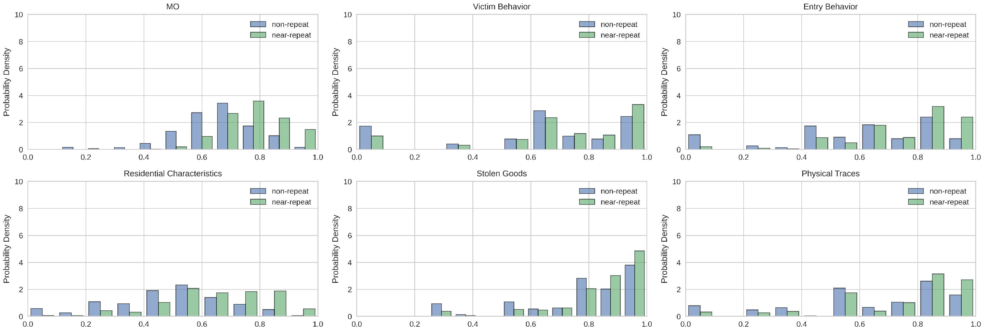
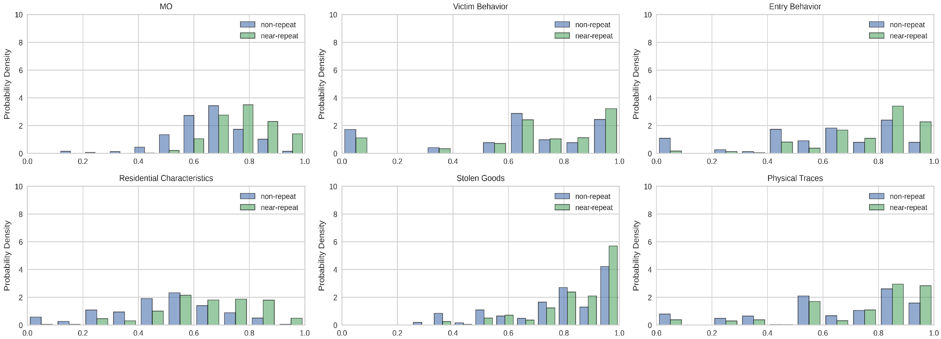
4.1. Distribution Comparison

After downsampling without replacement, the pairwise Jaccard index was plotted for near-repeat and non-repeat crimes as a histogram in Figure 1. The distribution of the Jaccard index for the MO, as well as the different MO subgroups, can be observed for both near-repeat and non-repeat crimes. As stated in Section 3, the Jaccard index is calculated using a pairwise comparison between crime scenes for both MO and the different subgroups. In Figure 1, near-repeat crimes often have a higher similarity score than non-repeats. This score difference in the distributions between near-repeats and non-repeats is further supported by the Wilcoxon test results. The Wilcoxon rank sum test revealed that for the overall MO there was a significant difference between near-repeat and non-repeat crimes ($U=21.4464$, $p<0.05$), $r=0.999$. Furthermore, differences were found between victim behavior for near-repeat and other crimes ($U=5.9097$, $p<0.05$, $r=0.999$), the behavior of the criminal when entering the residence for near-repeat versus other non-repeat crimes ($U=14.1083$, $p<0.05$, $r=0.999$), which type of residence targeted is different for near-repeat versus non-repeat crimes ($U=17.5485$, $p<0.05$, $r=0.999$), the type of goods stolen from repeat crime scenes versus non-repeat scenes ($U=7.3850$, $p<0.05$, $r=0.999$), and, finally, it was also found that the type of traces left at the crime scenes were different for the two classes ($U=8.1424$, $p<0.05$, $r=0.999$). Consequently, the results indicate the difference of the distributions and the feasibility to use the features as indicative of the classes. The results for an unbalanced dataset can be seen in Appendix A.

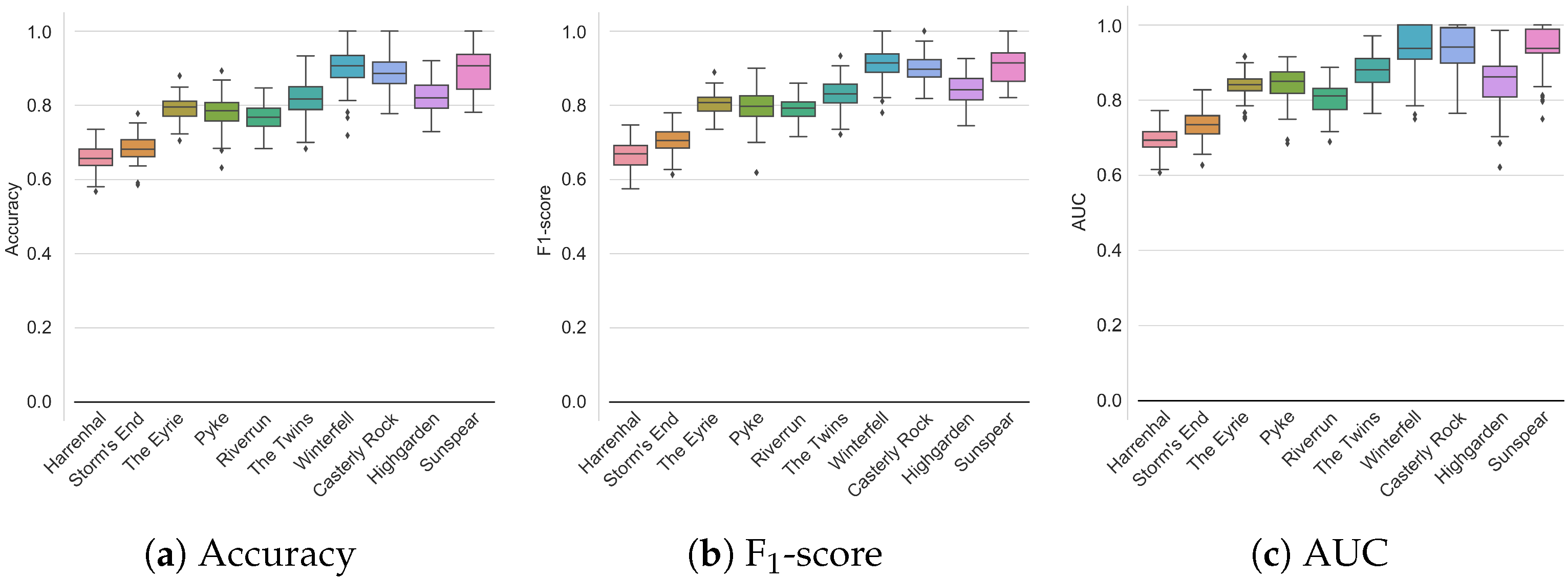
4.2. Near-Repeat Prediction

The experiments were conducted on a per city basis, as initial experiments over the complete geographical area proved unsuccessful (mean AUC around 0.55), being little better than chance. The results of the experiments presented in

Table 3. Prediction performance for the different cities.

City	AUC	Accuracy	F1-Score
Harrenhal	$0.6932$ ($0.0335)$	$0.6580$ ($0.0321$)	$0.6668$ ($0.0341$)
Storm’s End	$0.7337$ ($0.0344)$	$0.6842$ ($0.0326$)	$0.7043$ ($0.0303$)
the Eyrie	$0.8397$ ($0.0295)$	$0.7901$ ($0.0299$)	$0.8040$ ($0.0276$)
Pyke	$0.8443$ ($0.0430)$	$0.7820$ ($0.0445$)	$0.7952$ ($0.0435$)
Riverrun	$0.8057$ ($0.0393)$	$0.7676$ ($0.0345$)	$0.7894$ ($0.0296$)
the Twins	$0.8787$ ($0.0450)$	$0.8185$ ($0.0467$)	$0.8338$ ($0.0398$)
Winterfell	$0.9337$ ($0.0646)$	$0.8979$ ($0.0526$)	$0.9094$ ($0.0423$)
Casterly Rock	$0.9405$ ($0.0576)$	$0.8908$ ($0.0501$)	$0.9034$ ($0.0404$)
Highgarden	$0.8495$ ($0.0645)$	$0.8222$ ($0.0443$)	$0.8438$ ($0.0364$)
Sunspear	$0.9365$ ($0.0583)$	$0.8928$ ($0.0522$)	$0.9052$ ($0.0427$)
Mean	$0.8456$ ($0.0932)$	$0.8004$ ($0.0897)$	$0.8155$ ($0.0866$)

had an average F${}_1$-score of $0.81$ over all cities. Looking at individual cities, the F${}_1$-score ranged from $0.66$ (Harrenhal) to $0.90$ (Sunspear). Comparing prediction performance to city size, it seems that a bigger city corresponds to lower prediction performance. This is in part due to the fact that for the smaller cities fewer data points were available, but also because the demographic and environmental variables are much larger in a bigger city. The environmental variable changes between cities are supported by Figure 2, which shows that only a few select features for each label overlap between cities (and not necessarily the same features).

Further, the metrics do not vary much between each other. Observing Figure 3, the box-plots are compact. The size of the box-plots increases somewhat in cases where the data set is smaller (most noticeably in the case of Winterfell, The Twins, and Highgarden for AUC. As well as Sunspear for the F${}_1$-score). Overall, the box-plots (as well as the scores in Table 3) indicate that the models are capable of differentiating between near-repeat crimes and non-repeat crimes.

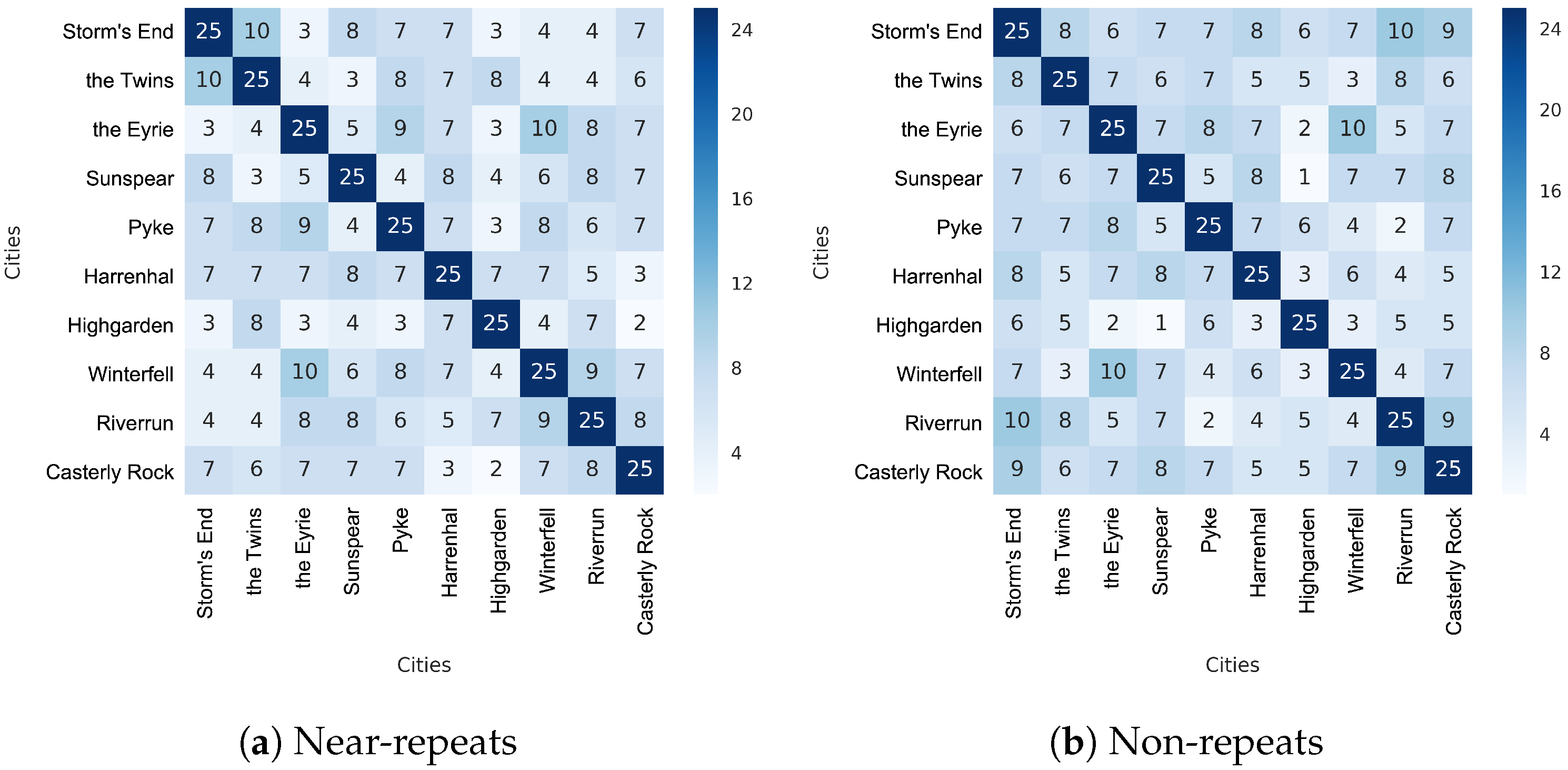
4.3. City Comparison

In order to compare cities, pairwise comparison of features between cities was conducted and the similarity index between each city was calculated. As such, the shared number of features between cities are shown. The results are presented in Figure 2. The figure shows the top 25 features indicative of either near-repeats (Figure 2a) or non-repeats (Figure 2b). Of 25 possible features, at most 10 were shared between cities. Often 6–7 features were shared between cities. The top shared features over all cities, indicative of non-repeats, were: windows are open/ventilating (shared by 7 of the 9 cities), household services (6), entered through cellar door (5), electronics stolen (5), fingerprint collected (5), medium-sized mark left while breaking in (5), clothes stolen (5), <5 marks left while breaking in (5), alarm activated (4), non-bulky goods stolen (4), bulky goods stolen (4), nothing stolen (4), trade announced/advertised by the victim (4), victim information N/A (4), vehicle keys stolen (4), other stolen goods (4), alarm sabotaged (4), entered through door (4), breaks window in to enter (4), triple-pane window on residence (4).

Similarly, the top features indicative of near-repeats were: misc. info not available (7), normal standard (6), view cover when entering (5), gloves used, (5), residents are active in neighbourhood watch (5), alarm disabled (5), townhouse (5), messy search during burglary (5), planned absence (4), residents home during crime (4), resident in company register (4), tips available (4), big mess during burglary (4), careful search during burglary (4), searchable goods stolen (4), entry through basement (4), witness exists (4), entry through mirror/patio door (4), entry on ground level (3), cash stolen (3).

Further, the temporal and spatial distribution of repeat and near-repeat crimes for the cities can be seen in Figure 4. The figure shows the number of near-repeat crimes for the possible values of temporal distance (0–14 days) and spatial distance (0–200 m). It indicates that the temporal distribution of crimes was not really consistent between cities. While some cities have too few crimes to draw any conclusions from, others indicate differences between the cities. One example of the latter is between The Eyrie and Harrenhall, where Harrenhall has two temporal peaks around 6 and 8 days, something that The Eyrie does not have. Similarly, for spatial comparisons, The Eyrie has a smaller increase of crimes around 100 m, which is not visible for Harrenhall or Storms End. Rather, it seems that the spatial distribution for Storms End and Harrenhall (and indeed all cities) have minor increases or decreases in the spatial distribution after the repeat crimes. However, while the differences are minor, they are still there and no city is identical to another. What is interesting though is the first spatial point after 0, i.e., at what distance do near-repeats start? This was very different between cities. In the case of The Eyrie, it was almost 20 m, but for e.g., Harrenhall it was closer to 10 m.

5. Analysis of Two Cities

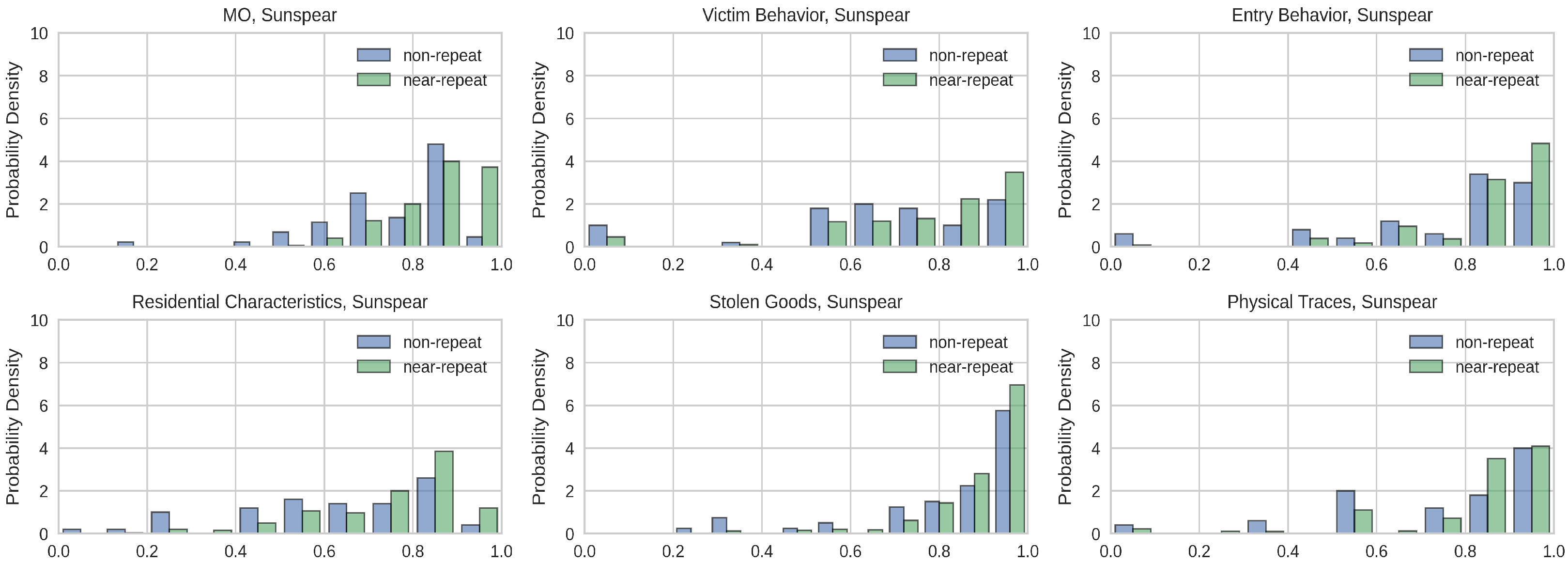
In this section, the results for two specific, randomly selected cities are presented and explored. Further, the important features are investigated in more detail.

5.1. Case: Sunspear

Figure 2 indicates that the number of shared features indicative of either near-repeats or non-repeats was quite low between cities. Of the top 25 features for each class, the mean number of shared features were approximately $6.5$. Consequently, it is difficult to draw general conclusions concerning what features impact near-repeat crimes. However, given the performance of the individual cities (as can be observed in Figure 3), local conclusions might be possible to find. This strengthens the claim that burglaries cluster locally with specific patterns. As such, one of the best performing cities, Sunspear, was selected to further exemplify the claim.

5.1.1. Distribution Comparison

Similar to Figure 1, the pairwise Jaccard index was plotted for near-repeat and non-repeat crimes for the chosen city and can be seen in Figure 5. The distribution of the Jaccard index for the different types of MO behaviour can be observed, with near-repeat crimes often having a higher similarity score than non-repeats. This score difference in the distributions between near-repeats and non-repeats is further supported by the Wilcoxon test results. The Wilcoxon rank sum test revealed that, for the overall MO, there was a significant difference between near-repeat and non-repeat crimes ($U=5.7006$, $p<0.05$), $r=0.999$. Furthermore, differences were found between victim behavior for near-repeat and other crimes ($U=3.1795$, $p<0.05$, $r=0.999$), the behavior of the criminal when entering the residence for near-repeat versus other non-repeat crimes ($U=2.7786$, $p<0.05$, $r=0.999$), which type of residence targeted is different for near-repeat versus non-repeat crimes ($U=4.4086$, $p<0.05$, $r=0.999$), the type of goods stolen from repeat crime scenes versus non-repeat scenes ($U=2.0553$, $p<0.05$, $r=0.999$), and, finally, it was also found that the type of traces left at the crime scenes were different for the two classes ($U=1.4265$, $p<0.05$, $r=0.999$). Consequently, the results indicate the difference of the distributions and reaffirm the feasibility of using the features as indicative of the classes.

5.1.2. Near-Repeat Prediction

Furthermore, the features for Sunspear were focused on. For each class, the mean coefficients, mean T-values and respective standard deviations were calculated and the features were ranked based on the T-values. The bottom and top 20% of features were then extracted and can be observed in

Table 4. Bottom and top 20% of features from Sunspear and their mean coefficients, mean T-values and respective standard deviations. Ranking based on T-value.

Feature ${}^{\mathit{d}}$	Mean Coefficient (SD)	Mean T-Value (SD)	Class
Alarm activated ${}^b$${}^c$	$-0.7767$ ($0.1147$)	$-5.1665$ ($0.8782$)	Not near-repeat
Non-bulky goods stolen ${}^b$${}^c$	$-0.4523$ ($0.0701$)	$-4.1137$ ($0.6651$)
Bulky goods stolen ${}^b$${}^c$	$-0.4757$ ($0.0871$)	$-3.7308$ ($0.6969$)
Large mark left ${}^b$${}^c$	$-0.6794$ ($0.1537$)	$-3.5342$ ($0.7919$)
Alcohol/tobacco stolen ${}^b$	$-0.3998$ ($0.1542$)	$-2.9088$ ($1.1269$)
Entry through cellar door ${}^b$${}^c$	$-0.6298$ ($0.1917$)	$-2.8388$ ($0.8700$)
Kids at home during burglary ${}^a$${}^c$	$-0.2216$ ($0.0865$)	$-2.7457$ ($1.0640$)
Active in neighbourhood watch ${}^a$	$-0.4981$ ($0.2188$)	$-2.7401$ ($1.1306$)
Small mark left ${}^b$${}^c$	$-0.6311$ ($0.1991$)	$-2.7378$ ($0.8737$)
Electronics stolen ${}^b$${}^c$	$-0.1546$ ($0.0434$)	$-2.6928$ ($0.8292$)
Drills used to enter ${}^b$	$-0.4692$ ($0.1307$)	$-2.5227$ ($0.7612$)
Fingerprint left ${}^b$	$-0.3382$ ($0.1580$)	$-2.3460$ ($1.0457$)
Nothing Stolen ${}^b$	$-0.2195$ ($0.0624$)	$-2.3413$ ($0.6946$)
Disabled/elderly targeted ${}^b$	$-0.2323$ ($0.1060$)	$-2.2571$ ($1.0111$)
View cover when entering ${}^b$	$0.2067$ ($0.1074$)	$1.9535$ ($1.002487$)	Near-repeat
Apartment at ground-level ${}^a$	$0.1480$ ($0.0655$)	$1.9882$ ($0.909634$)
Goods are searchable ${}^b$	$0.3005$ ($0.1263$)	$2.2747$ ($0.968793$)
Big mess during burglary ${}^b$	$0.3707$ ($0.1279$)	$2.2781$ ($0.796613$)
Messy burglary ${}^b$	$0.3616$ ($0.1068$)	$2.3431$ ($0.710198$)
DNA left ${}^b$	$0.5448$ ($0.2080$)	$2.4869$ ($0.920216$)
Entry through balcony door ${}^b$	$0.4211$ ($0.1450$)	$2.5742$ ($0.887874$)
Vehicle keys stolen ${}^b$	$0.2870$ ($0.0967$)	$2.6080$ ($0.876571$)
Unknown call prior ${}^b$${}^c$	$0.6182$ ($0.1391$)	$3.1245$ ($0.680689$)
Entry through basement ${}^b$${}^c$	$0.3739$ ($0.0956$)	$3.2171$ ($0.838424$)
Careful search during burglary ${}^b$${}^c$	$0.5141$ ($0.1160$)	$3.3135$ ($0.774788$)
Shoe print left ${}^b$${}^c$	$0.4005$ ($0.1393$)	$3.4098$ ($1.236385$)
Villa targeted ${}^a$${}^c$	$0.3405$ ($0.0825$)	$3.6257$ ($0.836176$)
Perfume stolen ${}^b$${}^c$	$0.9370$ ($0.0999$)	$8.4062$ ($0.883104$)

^a: features are environmental and not dependent on a crime taking place; ^b: features are dependent on a crime taking place; ^c: Mean p-value for the feature is p < 0.05; ^d: For each listed feature, Fishers combined probability test is 𝜒² < 0.05 and harmonic mean p-value is $\underset{}{\overset{˚}{p}}$ < 0.05.

.

Features indicative of near-repeats were (in order): perfume stolen, villa targeted, shoe-print left on scene, careful search during burglary, entry through basement, unknown call prior to burglary, vehicle keys stolen, entry through balcony door, D.N.A. left on scene, messy search of residence, very messy search of burglary, the stolen goods are searchable, the targeted apartment is at ground level, or the perpetrator had view cover when entering the residence. Besides unknown caller and vehicle keys stolen, the features seem to indicate that near-repeat crimes are targeting richer residences where the burglar can take their time to collect the goods.

A common denominator of the features of near-repeats seem to be opportunistic high reward crimes (and possibly low risk inferred by the perpetrator), with more highly valued (but difficult) goods being stolen, and DNA-marked or other searchable goods, perfume, or vehicle keys indicating certain targeting of goods. It also seems that the target residences and entry indicate a higher selectiveness; villas where the perpetrator enters through the balcony door or the basement, often with the view covered. Further, the residences are searched thoroughly (but messily).

However, a common denominator of the features of non-repeats seems to be quick crimes; easy entries, most often quick grab where the offender seems to behave rather riskily (and possibly having some rudimentary knowledge about the plaintiffs premises).

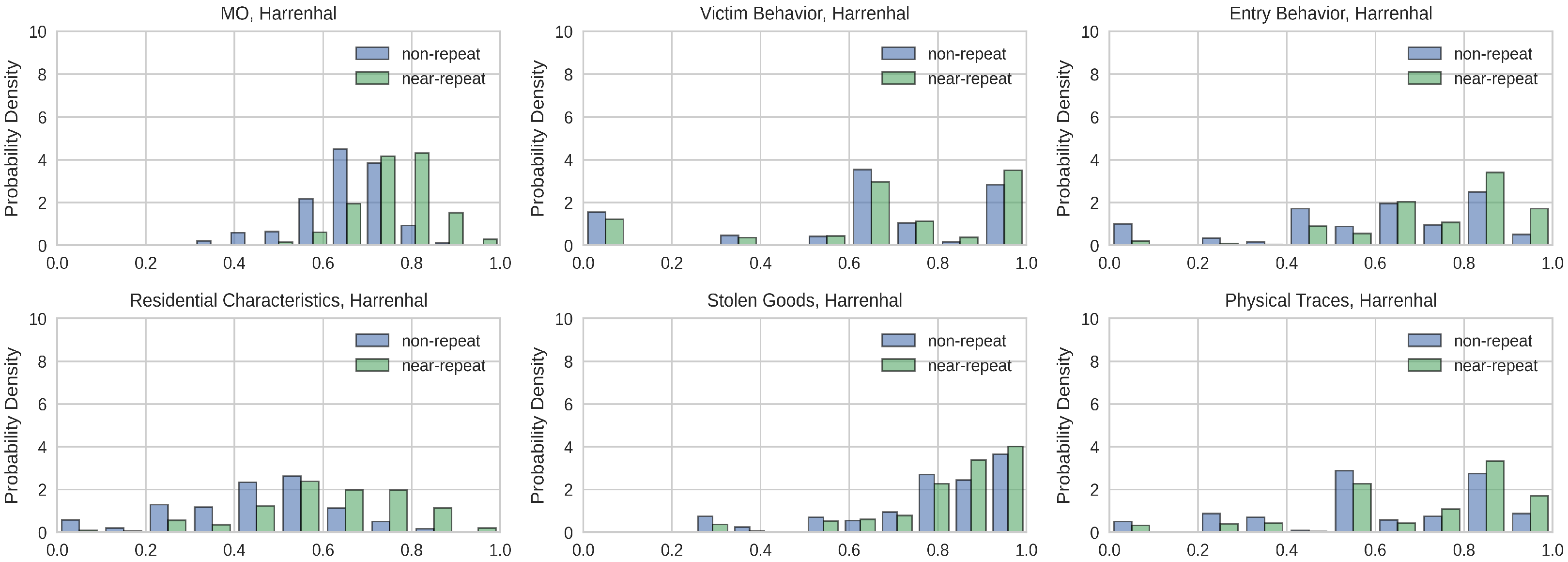
5.2. Case: Harrenhal

As a smaller city was investigated in detail, it is interesting to investigate if a larger city shows similar characteristics. Research indicates that this is likely not to be the case [2], something that is corroborated by Figure 2. Given that Harrenhal is one of the worst-performing cities (as can be observed in Figure 3), local conclusions might be possible to find.

5.2.1. Distribution Comparison

Similar to Figure 1, the pairwise Jaccard index was plotted for near-repeat and non-repeat crimes for the chosen city and can be seen in Figure 6. The distribution of the Jaccard index for the different types of MO behaviour can be observed, with non-repeat crimes often having a higher similarity score than near-repeats. This score difference in the distributions between near-repeats and non-repeats is further supported by the Wilcoxon test results. The Wilcoxon rank sum test revealed that for the overall MO there was a significant difference between near-repeat and non-repeat crimes ($U=15.4109$, $p<0.05$), $r=0.999$. Furthermore, differences were found between victim behavior for near-repeat and other crimes ($U=2.7118$, $p<0.05$, $r=0.999$), the behavior of the criminal when entering the residence for near-repeat versus other non-repeat crimes ($U=8.9706$, $p<0.05$, $r=0.999$), which type of residence targeted is different for near-repeat versus non-repeat crimes ($U=12.7021$, $p<0.05$, $r=0.999$), the type of goods stolen from repeat crime scenes versus non-repeat scenes ($U=2.8809$, $p<0.05$, $r=0.999$), and, finally, it was also found that the type of traces left at the crime scenes were different for the two classes ($U=5.3952$, $p<0.05$, $r=0.999$). Consequently, the results indicate the difference of the distributions and reaffirm the feasibility of using the features as indicative of the classes.

5.2.2. Near-Repeat Prediction

The features for Harrenhal were also focused on. For each class, the mean coefficients, mean T-values and respective standard deviations were calculated and the features were ranked based on the T-values. The bottom and top 20% of features were then extracted and can be observed in

Table 5. Bottom and top 20% of features from Harrenhal and their mean coefficients, mean T-values and respective standard deviations. Ranking based on T-value.

Feature ${}^{\mathit{d}}$	Mean Coefficient (SD)	Mean T-Value (SD)	Class
Victim owns company ${}^a$${}^c$	$-0.2141$ ($0.0136$)	$-4.3814$ ($0.2870$)	Not near-repeat
Ventilation window open ${}^a$${}^c$	$-0.3273$ ($0.0251$)	$-3.6180$ ($0.2881$)
Apartment at ground-level ${}^a$${}^c$	$-0.1902$ ($0.0190$)	$-3.3624$ ($0.3331$)
Alarm activated ${}^b$${}^c$	$-0.2197$ ($0.0250$)	$-3.1508$ ($0.3576$)
Medium marks left ${}^b$${}^c$	$-0.2732$ ($0.0276$)	$-3.1460$ ($0.3091$)
Single-level residence ${}^a$${}^c$	$-0.1419$ ($0.0207$)	$-2.6403$ ($0.3853$)
Weapons stolen ${}^b$${}^c$	$-0.5089$ ($0.0353$)	$-2.6208$ ($0.2298$)
Careful search during burglary ${}^b$${}^c$	$-0.2377$ ($0.0245$)	$-2.5297$ ($0.2596$)
Electronics stolen ${}^b$${}^c$	$-0.0757$ ($0.0111$)	$-2.5136$ ($0.3721$)
Vehicle on driveway during burglary ${}^b$${}^c$	$-0.1155$ ($0.0181$)	$-2.4344$ ($0.3898$)
Small marks left ${}^b$${}^c$	$-0.2062$ ($0.0258$)	$-2.4117$ ($0.2965$)
Triple-pane window on residence ${}^a$	$-0.1961$ ($0.0278$)	$-2.3974$ ($0.3446$)
=<5 marks left ${}^b$${}^c$	$-0.1649$ ($0.0218$)	$-2.3282$ ($0.3062$)
Large marks left ${}^b$${}^c$	$-0.2154$ ($0.0281$)	$-2.2686$ ($0.2957$)
Low standard residence ${}^a$	−2.9989 × ${10}^{10}$ (1.8334 × ${10}^{11}$)	$2.7075$ ($1.8910$)	Near-repeat
Drills used to enter ${}^b$${}^c$	$0.3485$ ($0.0434$)	$2.9345$ ($0.3399$)
Alcohol/tobacco stolen ${}^b$${}^c$	$0.2077$ ($0.0233$)	$2.9937$ ($0.3177$)
Victim in company register ${}^a$${}^c$	$0.1548$ ($0.0196$)	$3.0143$ ($0.3696$)
Glove prints left ${}^b$${}^c$	$0.1990$ ($0.0206$)	$3.0723$ ($0.3117$)
Victim uses household services ${}^a$${}^c$	$0.1828$ ($0.0172$)	$3.4481$ ($0.3208$)
Tips received ${}^b$${}^c$	$0.4442$ ($0.0451$)	$3.5123$ ($0.3191$)
Non-bulky goods stolen ${}^b$${}^c$	$0.2849$ ($0.0193$)	$3.8358$ ($0.2631$)
Passport/ID stolen ${}^b$${}^c$	$0.1951$ ($0.0182$)	$3.8429$ ($0.3494$)
Grass/Snow maintained ${}^a$${}^c$	$0.2554$ ($0.0228$)	$4.1159$ ($0.3579$)
Rental Apartment ${}^a$	−1.1740 × ${10}^9$ (1.3930 × ${10}^{11}$)	$4.1262$ ($2.6977$)
Bulky goods stolen ${}^b$${}^c$	$0.3393$ ($0.0211$)	$4.1756$ ($0.2617$)
Active in neighborhood watch ${}^a$${}^c$	$0.2584$ ($0.0224$)	$4.2181$ ($0.3575$)
Tool-marks left ${}^b$${}^c$	$0.3910$ ($0.0242$)	$6.0233$ ($0.3652$)

^a: features are environmental and not dependent on a crime taking place; ^b: features are dependent on a crime taking place; ^c: Mean p-value for the feature is p < 0.05; ^d: For each listed feature, Fishers combined probability test is 𝜒² < 0.05 and harmonic mean p-value is $\underset{}{\overset{˚}{p}}$ < 0.05.

.

A common denominator of the features of near-repeats seems to be opportunistic high reward crimes (and possibly low risk inferred by the perpetrator), including: drills used to enter, alcohol or tobacco stolen, victim in company register, glove prints left on site, victim uses household services, tips received, non-bulky goods stolen, passport or ID stolen, grass or snow maintained, bulky goods stolen, active in neighbourhood watch, tool-marks left. More highly valued (but difficult) goods seem to be stolen: passport or ID stolen, or alcohol or tobacco stolen. It also seems that the target residences and entry indicate a higher degree of planning: glove prints left on site, drills used to enter, both bulky and non-bulky goods were stolen. Further, features indicate a higher standard of residences or victims: victim in company register, victim uses household services, and active in neighbourhood watch.

It should be noted that two additional features were included for near-repeats in Table 5, but with a mean p-value greater than $0.05$: low standard of residence and rental apartment. While they had high T-values, they had negative coefficients, indicating a negative correlation with near-repeats. However, of 100 measurements, for low standard residence and rental apartment, 18 and 13 instances, respectively, had a coefficient <0 and contributed to the extreme means. For the low standard residence and rental apartment features, the harmonic means (https://docs.scipy.org/doc/scipy/reference/generated/scipy.stats.hmean.html, accessed on 19 February 2022) were $0.2559$ and $0.3013$, respectively.

Similarly to the features seen in Sunspear (Table 4), a common denominator of the features of non-repeats seems to be quick/impulsive crimes: easy entries, most often quick grab where the offender seems to behave rather riskily (and possibly having some rudimentary knowledge about the plaintiffs premises).

6. Discussion

Returning to the first research question—whether there are different characterizing features of near-repeat crimes as opposed to non-repeat crimes—we can conclude that there are. From the analysis, it is clear that near-repeat crimes are not the same type of crimes as non-repeat crimes. In other words, they show different empirical regularities. The Wilcoxon rank sum test revealed that there was a significant difference between near-repeat and non-repeat crimes for, e.g., the overall MO features ($U=21.4464$, $p<0.05$), $r=0.999$.

The second research question concerned to what extent near-repeat crimes can be predicted based on the features of the crime scene and the offenders MO. The results suggest that it is possible to reliably estimate, based on the characterizing features, the probability that a crime scene is part of a near-repeat crime chain, i.e., that another crime will take place within 500 m and within 14 days. The trained logistic regression models were able to correctly estimate classes in more than 80% of the cases.

Finally, the third research question investigated whether characterizing feature signatures for near-repeat crimes are different depending on spatial location. The results suggest that there is no general feature set indicating repeat crimes across cities. Rather, there is a heterogeneous set of features correlating with specific locations (cities). In other words, the MO signatures seem to be localized rather than generalizable across cities. This can be observed in Figure 2, where, on average, 6.5 (of 25) features were shared between cities.

6.1. Contributions

The contributions of this study are several. Firstly, methodologically, the number of observed burglaries was larger than in many previous studies. Moreover, the dataset was of high-resolution, including 137 features for every observed crime, containing both environmental and MO data. For instance, in studies of residential burglaries [45] used 160 pairs, containing 79 features, when investigating crime linkage.The authors of [61] investigated automated crime linkage versus manual crime linkage using 38 pairs of crime, of which only 8 were linked. Moreover, Ref. [47] investigated 650 linked crimes committed by 57 different offenders. Thus, the 685 near-repeat crimes and the 5059 non-repeat crimes together with 137 features for each instance provide a high-resolution dataset which, in turn, allowed for a more fine-grained approach than has been produced previously. It should be noted that most previous research has been conducted in an Anglosaxonian setting whereas the results in this study suggest the findings are applicable in a Swedish context as well.

Second, the study was not limited to analysis within a single city, but rather included several cities within a single country. The authors of [2] found that general crime patterns were similar at several spatial scales, but analysis at finer levels (such as street segments) showed significant variations within larger units, suggesting crime to be a rather localized phenomenon. Furthermore, Ref. [7] found considerable consistency in offenders behaviour across parameters for the crimes closest in space, even when there was separation in time spans. The results of this study suggest similar conclusions, with important amendments, i.e., it is possible to predict near repeat crimes on a higher spatial scale (e.g., city-level), but we also found that there are variations between cities. Previous research has suggested that offenders’ target selection is based on an existing (and evolving) awareness of the local space [24], which would support differences in MO between cities. As such, offenders are more likely to engage in burglaries in environments, and against targets, with which they are somewhat familiar or comfortable. The results are also somewhat supported by [20], which found that certain environmental variables might indicate crime likelihood, and that the environmental features might differ between cities as well. Finding the correct spatial scale when constructing models is important, but is something that is not investigated here. However, an initial investigation of the spatio-temporal bandwidth has been conducted by Chainey and Silva [6].

The features that were picked by the models indicate that repeat crime scenes are crimes where the offender is able to gain access and then acquire expensive items quickly. This highlights the need of theorizing about criminal behaviour as an individual (or individuals) in a spatio-temporal context, rather than focusing on either the individual or the context. Easy access and prevalence of expensive items most likely create a low-risk calculus (cf. [25]) and is in accordance with both rational and semi-rational accounts of criminal behaviour [27,62]. However, the inner workings of offenders can only be inferred via how the offender interprets the contextual cues that are present at the time for committing the crime (otherwise such a low-risk calculus cannot be made). Consequently, focusing on contextual cues, aligned with routine activity theory [26,27], such as location, time, particularities of the housing, or the presence of guardians, is equally important to combat crime. Thus, in order to avoid repeat crimes, the first step is to remove the opportunity for easy residential burglaries. This might be more easily said than done, but the characteristics indicative of near-repeat crimes are also indicators that overlap with how to improve security in homes that might otherwise be candidates for repeat crimes.

Given the possibility to predict whether a crime will soon be followed by another crime nearby, allows law enforcement to adjust resources accordingly. If the crime scene data indicates an elevated chance of another crime taking place nearby, police presence can be increased in the neighbourhood or neighbourhood watches can be informed to increase local vigilance. As such, it is possible that a higher number of residential burglaries can be avoided with the currently available resources.

Currently, Swedish law enforcement agencies have certain guidelines, or provide advice, for reducing residential burglaries when traveling (Bostadsinbrott-skydda dig, https://polisen.se/Utsatt-for-brott/Skydda-dig-mot-brott/Stold-och-inbrott/Bostadsinbrott/, accessed on 19 February 2022). This advice is, e.g., to have a dog or dog sign (currently omitted as per latest access), or for residents to park their car on the driveway. There is also advice that corresponds to features indicative of near-repeat crimes that are not statistically significant, e.g., ask a neighbour to cut the lawn, or remove snow if travelling for an extended time ($T=2.6208\left(0.3563\right)$), use an external light ($T=0.1878\left(0.8863\right)$), i.e., ”have lights routinely and randomly turned on and off outside the house”, have someone empty the mail ($T=0.9681\left(0.880\right)$). These are pieces of advice that are present in the indicator features for repeat crimes which, while not significant to the model, raise the probability of repeat crime.

Does this mean that this is bad advice? Probably not. However, the advice come across as counterintuitive to prevailing practice. Given an investigation into the features of repeat crime scenes and non-repeat crime scenes, the advice should probably be combined with other crime preventive measures to have the desired effect. It should also be noted that exterior lighting ($T=-0.3977\left(0.3331\right)$), alarm signs ($T=-1.6493\left(0.2948\right)$) (mean p-value not significant), and DNA marked goods ($T=-0.5676\left(0.3083\right)$) are indicators of non-repeat crime scenes. These three features are also included in law enforcement tips for decreasing the chance of a residential burglary. While they might not decrease the chance of residential burglaries (this cannot be inferred from this data), they seem to decrease the chance of near-repeat crime scenes. Thus, advising on how to avoid non-repeat and repeat crime should not typically follow the same type of advice.

Finally, the methodology described in this paper can be used in a decision support system for law enforcement with multiple goals. Firstly, it could be used to facilitate the management of resources. As described above, the use of this methodology would aid in locating areas where law enforcement should focus resources when combating burglaries. In combination with a hot-spot analysis or temporal analysis (e.g., aoristic analysis [63]), increased spatial and temporal focus may be achieved. Second, up-to-date directions to neighbourhood watch groups and other local organizations may be issued. This could be advisable to consider in city planning or advice on how residential owners should behave. Third, trend analysis of criminals behaviour can be analyzed in a much more detailed way than before, with a focus on MO characteristics. Trend analysis can be performed to detect differences in MOs in a national, regional or specific geographical area, but also with different temporal divisions, e.g., how trends differ from year to year, or over different seasons.

6.2. Avenues for Future Research

Temporal order was not evaluated in this study, i.e., the logistic regression model did not take into consideration the order of the crimes. However, one may wonder if there are differences between the first and second crime scene in a set of near-repeats? It could be that the order of crimes can highlight features that might be indicative of near-repeats. Or can features in non-repeat crime scenes be emulated in near-repeat residences to avoid near-repeats? That is, given the findings on non-repeat features, can neighbourhoods mimic certain features in order to reduce the risk of future near-repeat crimes occurring? Advice for preventing burglaries is already available, but might be on a too general level. Another interesting avenue for future research is to predict whether (dis)similarities in housing predict near-repeat and non-repeat crimes. A particular MO may be a consequence of particular housing homogeneity rather than a consequence of the offenders tactics.

Furthermore, in this study the temporal and spatial differences indicating repeat crimes were fixed. Future research could address the appropriateness of the spatial and temporal frame of near repeats. In fact, initial research has already been conducted by [6]. The spatial and temporal bandwidth, as denoted by [6], might differ from country to country, but also between regions in a country, e.g., between urban and rural environments. For example, spatial bandwidths in Sweden might differ between Lapland (the northern, less populated part of Sweden), Stockholm and Skåne (more densely populated). Further, the spatial and temporal bandwidths might differ between e.g., Sweden (population density of $24.1$ persons per km${}^2$, midyear population density of 2016 according to U.S. Census Bureau, https://www.census.gov/programs-surveys/international-programs/data/tools/international-data-base.html, accessed on 19 February 2022) and the Netherlands (population density of $502.1$ persons per km${}^2$).

It would also be interesting to investigate if MO features are indicative of near-repeat crimes being committed by the same offender, or if the offender has been affected in their behaviour by a previous offender (i.e., is criminal behaviour contagious?). In order to do so, it would be necessary to merge the dataset with data concerning criminal convictions and offender information.

7. Conclusions

Using data on 5744 residential burglaries with 137 features depicting MO, the differences between near-repeat and non-repeat crimes were investigated. Regression models were trained on crimes from 10 different cities in Sweden. The results indicate the possibility of estimating whether a crime was part of a near-repeat crime or not with a mean F${}_1$-score of $0.8155$ ($0.0866$). Furthermore, using logistic regression models, features indicative of the two classes (near-repeat and non-repeats) were extracted. Consequently, law enforcement officers can, using the model, estimate the likelihood that a crime scene is part of a near-repeat chain and increase law enforcement presence in areas likely to have a heightened risk profile of near-repeat crimes.

Further, the findings have policy implications, in that near repeats and other types of burglary must not necessarily follow the same type of advice regarding potential countermeasures, i.e., while the results indicate that near-repeats can be predicted in cities, the MO which indicates these differ between cities, making it difficult to provide general models and advice.

As discussed in Section 6.2, future work could include investigating dynamic bandwidths over different areas. The temporal order between crime pairs might also indicate that certain features are indicative of initial near-repeat crimes, for instance, if there are certain features that are associated with initiation of a near-repeat crime area, or features indicative of the last near-repeat. Finally, it would be interesting to investigate at what city size it is useful to start making divisions into parts of a city.

References

1. Quetelet, A. Sur L’Homme et le Développement de ses Facultés ou Essai de Physique Sociale; Bachelier, Imprimeur-Libraire: Paris, France, 1835; Volume 1, p. 1835. [Google Scholar]
2. Andresen, M.A.; Malleson, N. Spatial Heterogeneity in Crime Analysis. In Crime Modeling and Mapping Using Geospatial Technologies; Springer: Dordrecht, The Netherlands, 2013; pp. 3–23. [Google Scholar]
3. Bowers, K.J.; Johnson, S.D.; Pease, K. Prospective Hot-Spotting The Future of Crime Mapping? Br. J. Criminol. 2004, 44, 641–658. [Google Scholar] [CrossRef]
4. Johnson, S.D.; Bernasco, W.; Bowers, K.J.; Elffers, H.; Ratcliffe, J.; Rengert, G.; Townsley, M. Space–Time Patterns of Risk: A Cross National Assessment of Residential Burglary Victimization. J. Quant. Criminol. 2007, 23, 201–219. [Google Scholar] [CrossRef] [Green Version]
5. Bernasco, W.; Johnson, S.D.; Ruiter, S. Learning where to offend: Effects of past on future burglary locations. Appl. Geogr. 2015, 60, 120–129. [Google Scholar] [CrossRef] [Green Version]
6. Chainey, S.P.; Silva, B.F.A. Examining the extent of repeat and near repeat victimisation of domestic burglaries in Belo Horizonte, Brazil. Crime Sci. 2016, 5, 1. [Google Scholar] [CrossRef] [Green Version]
7. Johnson, D. The space/time behaviour of dwelling burglars: Finding near repeat patterns in serial offender data. Appl. Geogr. 2013, 41, 139–146. [Google Scholar] [CrossRef]
8. Wang, Z.; Liu, X. Analysis of burglary hot spots and near-repeat victimization in a large Chinese city. ISPRS Int. J. Geo-Inf. 2017, 6, 148. [Google Scholar] [CrossRef] [Green Version]
9. Rossmo, K. Geographic Profiling; CRC Press: Boca Raton, FL, USA, 1999. [Google Scholar]
10. Song, C.; Qu, Z.; Blumm, N.; Barabási, A.L. Limits of Predictability in Human Mobility. Science 2010, 327, 1018–1021. [Google Scholar] [CrossRef] [PubMed] [Green Version]
11. Chainey, S.P.; Curtis-Ham, S.J.; Evans, R.M.; Burns, G.J. Examining the extent to which repeat and near repeat patterns can prevent crime. Polic. An Int. J. 2018, 41, 608–622. [Google Scholar] [CrossRef]
12. Oatley, G.; Ewart, B.; Zeleznikow, J. Decision support systems for police: Lessons from the application of data mining techniques to “soft” forensic evidence. Artif. Intell. Law 2006, 14, 35–100. [Google Scholar] [CrossRef]
13. Roman, J.; Reid, S.; Reid, J.; Chalfin, A.; Adams, W.; Knight, C. The DNA Field Experiment: Cost-Effectiveness Analysis of the Use of DNA in the Investigation of High-Volume Crimes. 2008. Available online: https://www.ojp.gov/pdffiles1/nij/grants/222318.pdf (accessed on 31 January 2022).
14. O’Hara, C.; O’Hara, G. Fundamentals of Criminal Investigation, 7th ed.; Charles C Thomas Publisher Ltd.: Springfield, IL, USA, 1956. [Google Scholar]
15. Woodhams, J.; Hollin, C.R.; Bull, R. The psychology of linking crimes: A review of the evidence. Leg. Criminol. Psychol. 2010, 12, 233–249. [Google Scholar] [CrossRef]
16. Bennell, C.; Jones, N.J.; Melnyk, T. Addressing problems with traditional crime linking methods using receiver operating characteristic analysis. Leg. Criminol. Psychol. 2010, 14, 293–310. [Google Scholar] [CrossRef]
17. Tonkin, M.; Woodhams, J.; Bull, R.; Bond, J.W.; Palmer, E.J. Linking Different Types of Crime Using Geographical and Temporal Proximity. Crim. Justice Behav. 2011, 38, 1069–1088. [Google Scholar] [CrossRef]
18. Godwin, M. Reliability, Validity, and Utility of Criminal Profiling Typologies. J. Police Crim. Psychol. 2002, 17, 1–18. [Google Scholar] [CrossRef]
19. Boldt, M.; Borg, A.; Svensson, M.; Hildeby, J. Predicting burglars’ risk exposure and level of pre-crime preparation using crime scene data. Intell. Data Anal. 2018, 22, 167–190. [Google Scholar] [CrossRef]
20. Vandeviver, C.; Neutens, T.; Van Daele, S.; Geurts, D.; Vander Beken, T. A discrete spatial choice model of burglary target selection at the house-level. Appl. Geogr. 2015, 64, 24–34. [Google Scholar] [CrossRef] [Green Version]
21. Bowers, K.J.; Johnson, S.D. Who commits near repeats? A test of the boost explanation. West. Criminol. Rev. 2004, 5, 12–24. [Google Scholar]
22. Glaeser, E.L.; Sacerdote, B.; Scheinkman, J.A. Crime and social interactions. Q. J. Econ. 1996, 111, 507–548. [Google Scholar] [CrossRef] [Green Version]
23. Reich, B.; Porter, M. Partially supervised spatiotemporal clustering for burglary crime series identification. J. R. Stat. Soc. Ser. A Stat. Soc. 2015, 178, 465–480. [Google Scholar] [CrossRef] [Green Version]
24. Brantingham, P.; Brantingham, P. Crime pattern theory. In Environmental Criminology and Crime Analysis; Willan: London, UK, 2013; pp. 100–116. [Google Scholar]
25. Becker, G.S. Crime and Punishment: An Economic Approach. In The Economic Dimensions of Crime; Palgrave Macmillan UK: London, UK, 1968; pp. 13–68. [Google Scholar]
26. Cohen, L.E.; Felson, M. Social Change and Crime Rate Trends: A Routine Activity Approach. Am. Sociol. Rev. 1979, 44, 588. [Google Scholar] [CrossRef]
27. Clarke, R.V.; Felson, M. Introduction: Criminology, Routine Activity, and Rational Choice. Routine Act. Ration. Choice Adv. Criminol. Theory 1993, 5, 1–14. [Google Scholar]
28. Brantingham, P.L.; Brantingham, P.J. Environment, Routine, and Situation: Toward a Pattern Theory of Crime. Routine Act. Ration. Choice 1993, 5, 259. [Google Scholar]
29. Johnson, S.D.; Bowers, K.J.; Birks, D.J.; Pease, K. Predictive Mapping of Crime by ProMap: Accuracy, Units of Analysis, and the Environmental Backcloth. In Putting Crime in its Place; Springer New York: New York, NY, USA, 2009; pp. 171–198. [Google Scholar]
30. Lammers, M.; Menting, B.; Ruiter, S.; Bernasco, W. Biting once, twice: The influence of prior on subsequent crime location choice. Criminology 2015, 53, 309–329. [Google Scholar] [CrossRef]
31. Glaeser, E.L.; Sacerdote, B.I.; Scheinkman, J.A. The social multiplier. J. Eur. Econ. Assoc. 2003, 1, 345–353. [Google Scholar] [CrossRef]
32. Townsley, M.; Homel, R.; Chaseling, J. Infectious Burglaries. A Test of the Near Repeat Hypothesis. Br. J. Criminol. 2003, 43, 615–633. [Google Scholar] [CrossRef]
33. Farrell, G.; Pease, K. Once Bitten, Twice Bitten: Repeat Victimisation and Its Implications for Crime Prevention; Crime Prevention Unit, Paper 46; Home Office Police Research Group: London, UK, 1993.
34. Andresen, M.A.; Malleson, N. Testing the stability of crime patterns: Implications for theory and policy. J. Res. Crime Delinq. 2011, 48, 58–82. [Google Scholar] [CrossRef]
35. Andresen, M.A.; Linning, S.J. The (in) appropriateness of aggregating across crime types. Appl. Geogr. 2012, 35, 275–282. [Google Scholar] [CrossRef]
36. Weisburd, D.; Amram, S. The law of concentrations of crime at place: The case of Tel Aviv-Jaffa. Police Pract. Res. 2014, 15, 101–114. [Google Scholar] [CrossRef]
37. Hu, Y.; Wang, F.; Guin, C.; Zhu, H. A spatio-temporal kernel density estimation framework for predictive crime hotspot mapping and evaluation. Appl. Geogr. 2018, 99, 89–97. [Google Scholar] [CrossRef]
38. Xue, Y.; Brown, D.E. A decision model for spatial site selection by criminals: A foundation for law enforcement decision support. Syst. Man Cybern. Part C Appl. Rev. IEEE Trans. 2003, 33, 78–85. [Google Scholar]
39. Wang, S.; Li, X.; Cai, Y.; Tian, J. Spatial and temporal distribution and statistic method applied in crime events analysis. In Proceedings of the 2011 19th International Conference on Geoinformatics, Shanghai, China, 24–26 June 2011; pp. 1–6. [Google Scholar]
40. Zhou, G.; Lin, J.; Zheng, W. A web-based geographical information system for crime mapping and decision support. In Proceedings of the 2012 International Conference on Computational Problem-Solving (ICCP), Leshan, China, 19–21 October 2012; pp. 147–150. [Google Scholar]
41. Phillips, P.; Lee, I. Crime analysis through spatial areal aggregated density patterns. Geoinformatica 2011, 15, 49–74. [Google Scholar] [CrossRef]
42. Chainey, S.; Ratcliffe, J. GIS and Crime Mapping; John Wiley & Sons, Ltd.: Hoboken, NJ, USA, 2005. [Google Scholar]
43. Glasner, P.; Leitner, M. Evaluating the impact the weekday has on near-repeat victimization: A spatio-temporal analysis of street robberies in the city of Vienna, Austria. ISPRS Int. J. Geo-Inf. 2017, 6, 3. [Google Scholar] [CrossRef] [Green Version]
44. Sagovsky, A.; Johnson, S.D. When Does Repeat Burglary Victimisation Occur? Aust. N. Z. J. Criminol. 2007, 40, 1–26. [Google Scholar] [CrossRef]
45. Markson, L.; Woodhams, J.; Bond, J.W. Linking serial residential burglary: Comparing the utility of modus operandi behaviours, geographical proximity, and temporal proximity. J. Invest. Psychol. Offender Profiling 2010, 7, 91–107. [Google Scholar] [CrossRef]
46. Martin, G. A Game of Thrones (A Song of Ice and Fire, Book 1); A Song of Ice and Fire, HarperCollins Publishers: London, UK, 2010. [Google Scholar]
47. Bennell, C.; Jones, N.J. Between a ROC and a hard place: A method for linking serial burglaries bymodus operandi. J. Investig. Psychol. Offender Profiling 2005, 2, 23–41. [Google Scholar] [CrossRef]
48. Sheskin, D. Handbook of Parametric and Nonparametric Statistical Procedures; Chapman & Hall: Boca Raton, FL, USA, 2007. [Google Scholar]
49. Wendt, H.W. Dealing with a common problem in Social science: A simplified rank-biserial coefficient of correlation based on the U statistic. Eur. J. Soc. Psychol. 1972, 2, 463–465. [Google Scholar] [CrossRef]
50. Cohen, J. Statistical Power Analysis for the Behavioral Sciences; Taylor & Francis: New York, NY, USA, 2013. [Google Scholar]
51. Flach, P. Machine Learning: The Art and Science of Algorithms that Make Sense of Data; Cambridge University Press: Cambridge, UK, 2012. [Google Scholar]
52. Rogati, M.; Yang, Y. High-performing feature selection for text classification. In Proceedings of the Eleventh International Conference on Information and Knowledge Management, McLean, VA, USA, 4–9 November 2002; pp. 659–661. [Google Scholar]
53. Yang, Y.; Pedersen, J. A comparative study on feature selection in text categorization. ICML 1997, 97, 412–421. [Google Scholar]
54. Liu, H.; Motoda, H. Feature Selection for Knowledge Discovery and Data Mining; The Springer International Series in Engineering and Computer Science; Springer: Boston, MA, USA, 2012. [Google Scholar]
55. Fisher, R.A. Statistical methods for research workers. In Breakthroughs in Statistics; Springer: New York, NY, USA, 1992; pp. 66–70. [Google Scholar]
56. Wilson, D.J. The harmonic mean p-value for combining dependent tests. Proc. Natl. Acad. Sci. USA 2019, 116, 1195–1200. [Google Scholar] [CrossRef] [Green Version]
57. Witten, I.H.; Frank, E. Data Mining: Practical Machine Learning Tools and Techniques; Morgan Kaufmann Publications: San Francisco, CA, USA, 2005. [Google Scholar]
58. Steyerberg, E.W.; Harrell, F.E., Jr.; Borsboom, G.; Eijkemans, M.J.C.; Vergouwe, Y.; Habbema, J.D.F. Internal validation of predictive models: Efficiency of some procedures for logistic regression analysis. J. Clin. Epidemiol. 2001, 54, 774–781. [Google Scholar] [CrossRef]
59. Harrell, F.E. Regression Modeling Strategies: With Applications to Linear Models, Logistic Regression, and Survival Analysis; Springer: Cham, Switzerland, 2001. [Google Scholar]
60. Fawcett, T. An introduction to ROC analysis. Pattern Recognit. Lett. 2006, 27, 861–874. [Google Scholar] [CrossRef]
61. Bennell, C.; Bloomfield, S.; Snook, B.; Taylor, P.; Barnes, C. Linkage analysis in cases of serial burglary: Comparing the performance of university students, police professionals, and a logistic regression model. Psychol. Crime Law 2010, 16, 507–524. [Google Scholar] [CrossRef] [Green Version]
62. Cromwell, P.F.; Olson, J.N.; Avary, D.W. Breaking and Entering: An Ethnographic Analysis of Burglary; Sage: Newbury Park, CA, USA, 1991; Volume 8. [Google Scholar]
63. Ratcliffe, J.H. Aoristic Signatures and the Spatio-Temporal Analysis of High Volume Crime Patterns. J. Quant. Criminol. 2002, 18, 23–43. [Google Scholar] [CrossRef]
Figure 1. Histogram of the distribution between near-repeats and other residential burglaries for different MO behaviour, based on a balanced data set. The X-axis denotes the Jaccard index, and the Y-axis the probability density.
Ijgi 11 00160 g001
Figure 2. The number of shared features of the top 25 features per city. Please note that the city order differs from other figures and tables.
Ijgi 11 00160 g002
Figure 3. Box plots for the AUC, Accuracy, and F 1 -score for the cities. This indicates the spread of the evaluation metrics for the different cities.
Ijgi 11 00160 g003
Figure 4. The spatial and temporal distribution of crimes per city. The y-axis denotes the number of crimes. Please note that the y-axis differs between sub-plots.
Ijgi 11 00160 g004
Figure 5. The distribution between near-repeats and other residential burglaries for different MO behaviour for the city Sunspear.
Ijgi 11 00160 g005
Figure 6. The distribution between near-repeats and other residential burglaries for different MO behaviour for the city Harrenhal.
Ijgi 11 00160 g006