Attention-Based Multiscale Spatiotemporal Network for Traffic Forecast with Fusion of External Factors

Abstract

Periodic traffic prediction and analysis is essential for urbanisation and intelligent transportation systems (ITS). However, traffic prediction is challenging due to the nonlinear flow of traffic and its interdependencies on spatiotemporal features. Traffic flow has a long-term dependence on temporal features and a short-term dependence on local and global spatial features. It is strongly influenced by external factors such as weather and points of interest. Existing models consider long-term and short-term predictions in Euclidean space. In this paper, we design an attention-based encoder–decoder with stacked layers of LSTM to analyse multiscale spatiotemporal dependencies in non-Euclidean space to forecast traffic. The attention weights are obtained adaptively and external factors are fused with the output of the decoder to evaluate region-wide traffic predictions. Extensive experiments are conducted to evaluate the performance of the proposed attention-based non-Euclidean spatiotemporal network (ANST) on real-world datasets. The proposed model has improved prediction accuracy over previous methods. The insights obtained from traffic prediction would be beneficial for daily commutation and logistics.

1. Introduction

Rapid urbanisation has introduced significant changes in transportation and mobility patterns, causing threats to traffic congestion. This could be mitigated with the use of intelligent systems for transportation, which are vital for smart mobility, traffic control and route guidance. Accurate traffic prediction assists people in planning travel routes, reduces commutation cost/time and alleviates traffic congestion. Traffic flow is the number of vehicles that pass through a road during a specific periodic interval. When the time span is from a few seconds to an hour, it can be categorised as a short-term forecast. However, long-term forecast targets predict traffic flow in the future over the course of one or more days, weeks or months [1,2]. In general, traffic flow is categorised as a type of time-series which is stochastic and nonlinear and made up of continuous valued measurements taken periodically. Stationary time-series data do not depend on trends and seasons. Traffic data are non stationary, being dependent on both trends and seasons. Likewise, time-series forecasts can be univariate if only the previous values of the series are employed to predict the future or multivariate if predictors are dependent of the previous values and other variables. Time-series forecasting [3,4] has been effectively used in traffic analysis to predict short-term and long-term future traffic flows with high accuracy. Traffic flow prediction can be used to analyse the traffic flow data to forecast future traffic.

Numerous studies in the literature have been conducted on short-term traffic forecasting. However, this time scale places constraints on travellers when making decisions in order to avoid traffic congestion. Precise and well-timed long-term forecasting can aid ITS managers in making wise and accurate decisions regarding traffic management and planning. Nevertheless, long-term forecasts are swayed by sensitive propagation errors. As the prediction horizon increases, the accuracy reduces, since most of the prediction methods are iterative, which causes the error to be accumulated and propagated, and which makes long-term forecasts more challenging than short-term forecasts. Likewise, traffic prediction can be based on links or regions. A majority of the literature has focused on traffic prediction with a single link [1,2,3,4,5,6,7,8,9,10,11,12], neglecting spatiotemporal dependencies. Nevertheless, few authors have considered all links of the network to have equal weightage. Practically, only certain significant links contribute to the network traffic, generating unique patterns over time. For example, certain busy links and junctions generate an enormous amount of traffic during peak hours, whereas other certain links are traffic-free. Therefore, network-wide traffic needs to be analysed for realistic results.

Owing to the applications of sensor technology, a huge volume of traffic data is available for research. Time-series analyses, exponential smoothing and machine learning approaches have been used for prediction. With the advent of deep learning, which is capable of learning features with less prior knowledge and artificial intelligence, information can be easily extracted from images and videos. Deep learning has a high prediction accuracy and solves problems that cannot be dealt with through conventional methods. In general, convolution neural networks (CNN) extract spatial features, but they are limited as they only use Euclidean data. Traffic road networks produce non-Euclidean data, and thus, graph convolution neural networks (GCN) are commonly deployed in traffic analyses [8,13]. To be more specific, a GCN has spectral methodologies and spatial-based approaches. Spectral-based approaches introduce filters for graph convolutions based on graph signal processing to remove noise. Furthermore, spatial-based approaches aggregate feature information from neighbours to form graph convolutions. However, the convolution operator in a GCN is not effective for non-Euclidean space correlation. Intrinsically, recurrent neural networks (RNN) are preferred while preprocessing time-series data. Unfortunately, the predominant vanishing gradient problem in RNNs limits their ability to learn long sequences, and thus, variants of RNN—long short-term memory (LSTM) and gated recurrent unit (GRU)—are used [14]. Nevertheless, for these variants, as the length of the input sequence increases, sequence models are deployed. An encoder–decoder mechanism is a type of sequence model that has been integrated with an RNN to predict traffic for large horizons. However, when the length of the input series increases, the performance of the network deteriorates. Hence, it is preferable to employ an attention mechanism with an encoder–decoder LSTM to capture spatiotemporal dependencies and improve prediction accuracy.

To be specific, traffic flow is dependent on multiscale global and local spatiotemporal dependencies. Consider Figure 1, in which the traffic flow at sensor 4 is directly influenced by the traffic flow at sensor 2 and sensor 3, which would cause a local spatial dependency. On the other hand, the traffic at sensor 1 indirectly affects the traffic at sensor 4, contributing to global spatial dependencies. Likewise, the traffic at time $t+1$ depends on the traffic at t and $t-1$ to depict weekly and daily patterns.

For instance, consider two stadiums that are semantically similar, where one stadium hosts an event while the other is not hosting anything. In this case, it is not possible to only consider the distance. Therefore, points of interest have to be considered for traffic prediction. However, traffic flow is directly influenced by weather. The key motivation of this paper is to address the challenges in traffic prediction considering spatiotemporal dependencies in non-Euclidean space along with the influence of external factors. The key contributions are as follows:

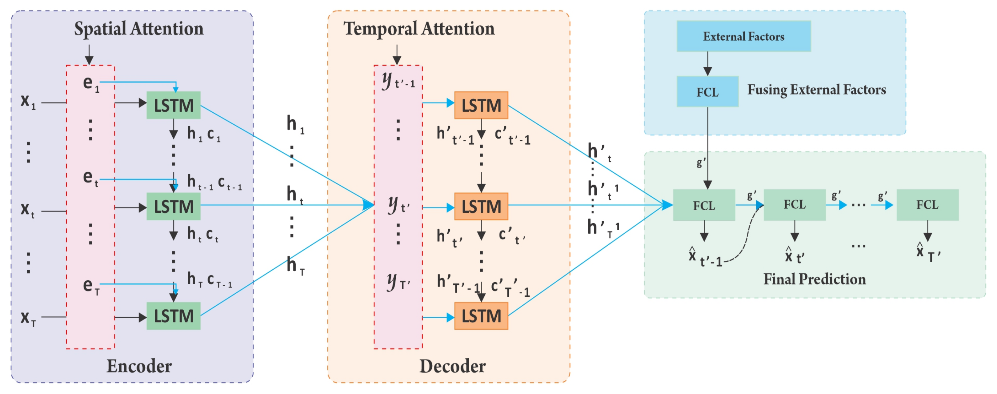
• The design of a region-based attentive encoder and decoder to capture multiscale spatial and temporal dependencies in non-Euclidean space.
• The design of a decision fusion model by concatenating the output of the decoder with external factors such as weather, holidays and points of interest to forecast the future traffic flow in a horizon.

Our work is different from existing works. Non-Euclidean structures with spatiotemporal features have been studied in [15,16,17,18,19]. However, the influence of external factors such as weather, which has a vast impact on traffic flow, has not been investigated in non-Euclidean space.

2. Related Work

In general, traffic flow considers speed, flow, and density over a period of time. These parameters are vital to the schedule and plan of the travel pattern. Traditional traffic flow prediction methods can be categorised into three types: model-driven, data-driven and hybrid models. These models are defined below:

• Model-driven or parametric models are based on several assumptions and preconditions, which include the Autoregressive Integrated Moving Average (ARIMA) model, Kalman filtering and Bayesian networks. The ARIMA model is known to predict stochastic traffic flow. The variants of the ARIMA model based on traffic flow are Kohonen ARIMA, subset ARIMA, seasonal ARIMA and time-series integrated ARIMA to predict short-term traffic [5,6,7]. The ARIMA model is a well-known and effective framework for traffic prediction. However, parametric models cannot fully represent the nonlinearity of traffic and extract spatiotemporal features.
• Data-driven or non-parametric models have made use of artificial intelligence to possibly manage big data when traffic flow changes dynamically [1,2]. Initially, non-parametric methods were based on machine learning. To forecast traffic, random forest, Support Vector Machine [20] and k-nearest neighbours (KNN) [21] were used. Recently, deep learning models, such as neural networks [2,22], deep belief networks (DBN) [23,24,25,26], CNNs [27,28], artificial neural networks (ANN) [29] and RNNs, [30,31,32] have been successful in short-term traffic forecasting. To overcome the limitations due to the vanishing gradient and exploding gradient problems occurring in RNN, an LSTM network [14,33,34,35] was deployed and found to have excellent prediction. Even though these models have considered the nonlinearity and stochastic nature of traffic flow, they are not effective for long-term prediction. However, long-term traffic is predicted using LSTM in [1] and deep neural network in [2]. To be specific, challenges persist in determining the accuracy and reliability of nonlinear, complex, time-varying systems. Nevertheless, recent literature has focused on non-Euclidean space to efficiently capture spatiotemporal features. The authors in [15] have proposed an attention-based periodic temporal neural network using LSTM to predict traffic in non-Euclidean space. Multigraph convolution network [16] has captured spatial and temporal dependencies with its extensive applications in GCN. However, external factors and weather are not considered.
• Hybrid or combined models integrate individual models to provide the benefits of both models when combined to improve estimation accuracy. It is significant that hybrid models are more accurate and effective in predicting the real-time flow of traffic. The authors in [11] have used DBN and multitask learning along with data fusion for weather to enhance the prediction accuracy. Data fusion enables the information from multiple sources to be combined together to produce high reliability. ARIMA and LSTM were combined to predict short-term traffic, achieving better accuracy in [12]. Likewise, [9] has jointly modelled CNN and LSTM based on Euclidean distance. Furthermore, in [8,9,10], spatial and temporal features are studied without taking into account external factors. Moreover, a hybrid model with CNN and LSTM has been used to predict the hourly air temperature in [17]. Likewise, multi-range attentive bicomponent GCN [18] and diffusion convolutional recurrent neural network (DCRNN) [19] have investigated non-Euclidean space with variants of CNN and GRU. Thus, hybrid models have improved accuracy over model-driven methods, and they are suitable for real-time traffic analysis.

It is obvious that data-driven models have received keen attention. On the contrary, hybrid models can realistically forecast traffic. While very few studies have explored external factors in hybrid models.

3. Problem Formulation

A region $\mathbb{R}$ has N links that are connected by junctions to make a network. Every link generates a time series sequence of traffic volumes at time t represented by $x^i=(x_1^i,x_2^i,\cdots ,x_t^i\cdots x_T^i)\in {\mathbb{R}}^T$. The traffic volume matrix is obtained by concatenating the time series vectors of all the N links in region $\mathbb{R}$ during time T:

$$\begin{array}{c}\hfill X_T^N=(x_1^1,x_2^2,\cdots ,x_t^i\cdots x_T^N)\in {\mathbb{R}}^{N\times T}\end{array}$$

(1)

In general, traffic flow is influenced by external factors such as weather. The weather condition of each link N at time t is represented by $x_t^i=(x_t^1,x_t^2,\cdots ,x_t^n)\in {\mathbb{R}}^T$. Therefore, representing the weather conditions of all N links in $\mathbb{R}$, as one of the input parameters, the weather matrix is generated:

$$\begin{array}{c}\hfill E_T^N=(x_t^1,x_t^2,\cdots ,x_T^N)\in {\mathbb{R}}^{N\times T}\end{array}$$

(2)

The objective is to forecast traffic volumes for future K horizons in $\mathbb{R}$ as in Equation (3), which is a fusion of the historical observations of traffic flow and weather ${\widehat{X}}_t=f_{fusion}(X_T^N,E_T^N)$:

$$\begin{array}{c}\hfill {\widehat{X}}_t={({\widehat{x}}_t,{\widehat{x}}_{t+1},\cdots ,{\widehat{x}}_{t+k})}^T\in {\mathbb{R}}^{K\times T}\end{array}$$

(3)

Table 1. Notations.

Notation	Description
$\mathbb{R}$	region
N	number of links in the region $\mathbb{R}$
$x_i\in {\mathbb{R}}^{\mathbb{T}}$	traffic volume of link i during the past time steps T
$X_T^N$	traffic volume of all N links in region $\mathbb{R}$
$E_T^N$	weather of all N links in region $\mathbb{R}$
${\widehat{X}}_t$	predicted traffic for future horizons
${\alpha }_t^i$	spatial weight of at time t for link i
$e_t\in \mathbb{R}$	spatial attention weight vector at t
M	spatial model dimension
L	dimension of LSTM encoder
$v_s$,$b_s$,$U_s$,$W_s$	learnable parameters in spatial model
P	dimension of decoder LSTM
Q	dimension of the temporal model
$v_d$,$b_d$,$U_d$,$W_d$	learnable parameters in temporal model
$y_{t^{\prime }}$	temporal context at $t^{\prime }$

lists the notations used in this paper.

4. Attention-Based Non-Euclidean Spatiotemporal Network (ANST)

ANST deploys the architecture of the encoder–decoder LSTM with an attention mechanism, as shown in Figure 2. The key components are as follows:

(i)

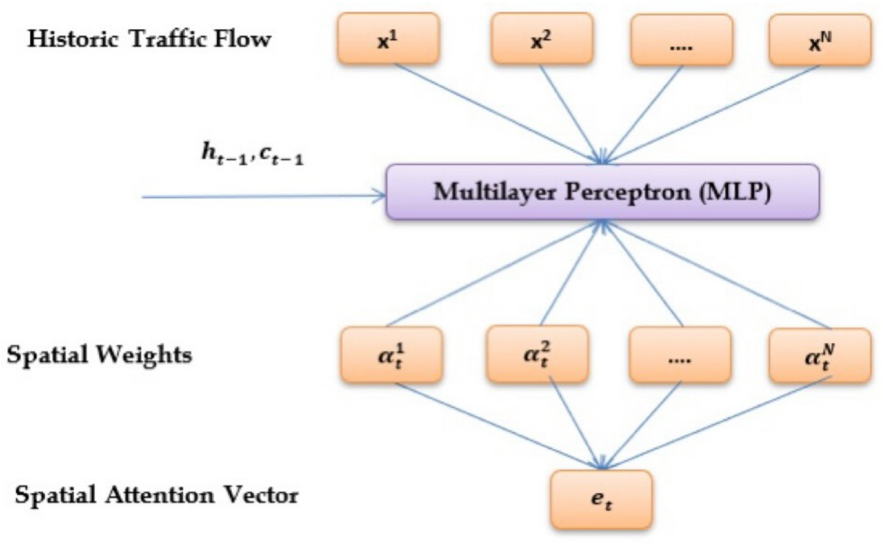
Encoder to model spatial dependencies: The encoder uses LSTM components to extract spatial dependencies from the historical input traffic data. The spatial attention weight vectors $({\alpha }_t^1,{\alpha }_t^2,\cdots ,{\alpha }_t^N)$ are calculated with the support of a multi-layer perceptron (MLP) layer, as shown in Figure 3. The weight vector $e_t$ is obtained at time t from the last hidden state $h_{t-1}$ and cell state $c_{t-1}$. The attention-based spatial non-Euclidean hidden states ($h_1,h_2,\cdots ,h_t$) are learned from the encoder and are fed as the input for the LSTM decoder to capture temporal dependencies.

(ii)

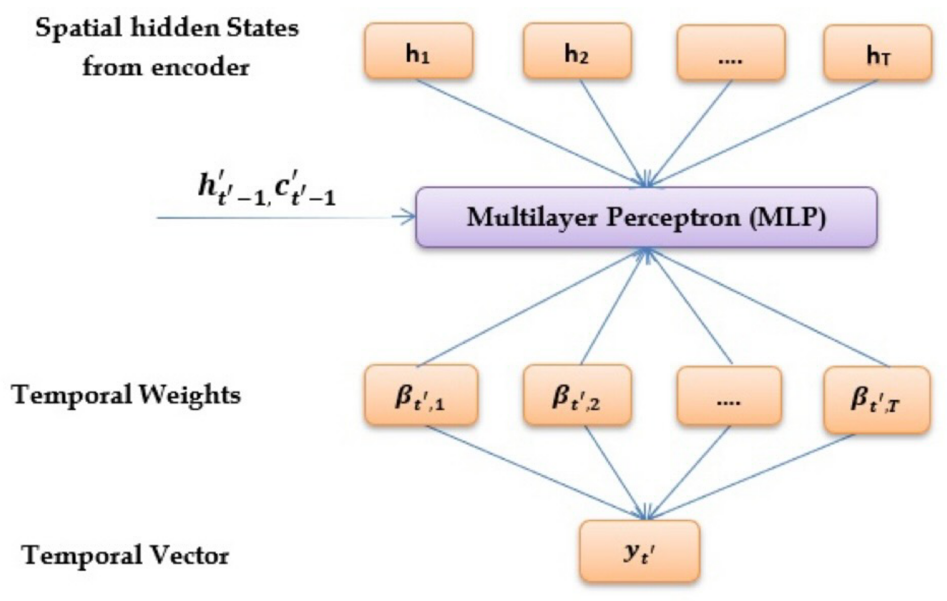
Decoder to model temporal dependencies: The decoder uses LSTM units to embed the spatial hidden states. The temporal weight vector ${\beta }_{t^{\prime }}$ is obtained at time $t^{\prime }$ from the last hidden state $h_{t-1}^{\prime }$ and cell state $c_{t-1}^{\prime }$. The temporal context $y_{t^{\prime }}$ is the summation of weights measured by the MLP layer and the non-Euclidean hidden states ($h_1,h_2,\cdots ,h_t$) from the encoder, as shown in Figure 4.

(iii)

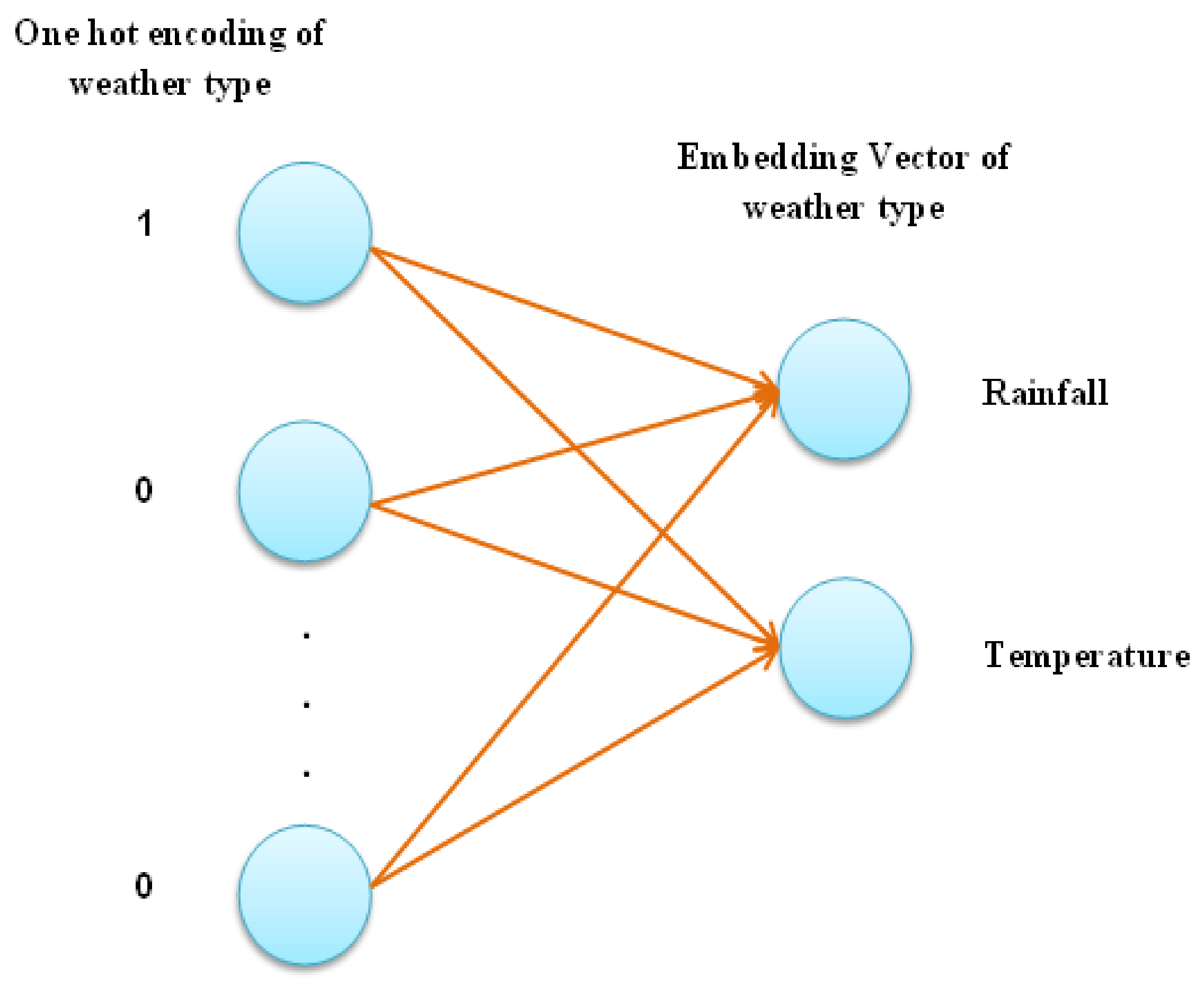
Data fusion for modelling weather and external factors: Data fusion integrates data from multiple sources to enrich the quality of information. Decision-in, decision-out fusion is performed with the weather data from Equation (2), along with the output of the decoder LSTM (16), to obtain an enhanced prediction.

4.1. Modelling Spatial Features with Attentive Encoder

Traffic flow prediction for a region depends upon the links. Generally, each individual link is considered, or equal weights are assigned to all the links. However, the traffic at each link is not the same, changes over time and is dependent upon external factors. Moreover, the links show spatial dependencies. For instance, the downstream traffic flow would depend on traffic flow at the intersections and upstream links, along with external events. In general, the spatial structure of the identified region is formulated as a matrix, where each entry corresponds to rectangular regions. As a result of the semantics and static distance between the nodes, a Euclidean structure is obtained. However, the static distance obtained would be inaccurate and lead to false conclusions. Therefore, attention mechanisms are deployed to capture spatial correlations by learning the assigned weights. ANST has used stacked layers of LSTM to capture multi-scale global and local spatial dependencies using dynamic attention weights derived from the previous cell state $c_{t-1}\in {\mathbb{R}}^M$ for each link i using Equation (4). To be more specific, the developed spatial attention model encapsulates spatial dependencies with LSTM and MLP:

$$\begin{array}{c}\hfill {\alpha }_t^i=v_s^{T}tanh(W^s[c_{t-1};h_{t-1}]+U_s{\left(x_i\right)}^T+b_s)\end{array}$$

(4)

where $v_s\in {\mathbb{R}}^L$, $b_s\in {\mathbb{R}}^L$, $W_s\in {\mathbb{R}}^{L\times 2M}$, $U_s\in {\mathbb{R}}^{L\times T}$ are the model parameters. Tanh is used as the activation function owing to its performance in handling the predominant vanishing gradient problem. The obtained spatial attention weight ${\alpha }_t^i$ is adaptive and normalised using the softmax function in Equation (5) such that the sum of all attention weights is one:

$$\begin{array}{c}\hfill {\alpha }_t^i=\frac{exp\left({\alpha }_t^i\right)}{{\displaystyle \sum _{j=1}^N}exp\left({\alpha }_t^i\right)}\end{array}$$

(5)

A significant change in traffic flow at time t in non-Euclidean space is obtained by concatenating the spatial attention weights to produce a column vector:

$$\begin{array}{c}\hfill e_t=(\alpha -t^1,\alpha -t^2,\cdots ,\alpha -t^N)\end{array}$$

(6)

The LSTM base model is enhanced to accommodate the attention mechanism weights $e_t$. The modified equations of LSTM with parameters $w_f,w_i,w_o,w_c\in {\mathbb{R}}^{M\times (M+2N)}$, and $b_f,b_i,b_o,b_c\in {\mathbb{R}}^M$ for forget gate, input gate, output gate, and memory cell with $\sigma$ as activation function are given in Equations (7)–(12):

$$\begin{array}{c}\hfill f_t=\sigma \left(W_f\right[h_{t-1};x_t;e_t]+b_f)\end{array}$$

(7)

$$\begin{array}{c}\hfill i_t=\sigma \left(W_i\right[h_{t-1};x_t;e_t]+b_i)\end{array}$$

(8)

$$\begin{array}{c}\hfill o_t=\sigma \left(W_o\right[h_{t-1};x_t;e_t]+b_o)\end{array}$$

(9)

$$\begin{array}{c}\hfill {\widehat{c}}_t=tanh\left(W_c\right[h_{t-1};x_t;e_t]+b_c\end{array}$$

(10)

$$\begin{array}{c}\hfill c_t=f_t\otimes c_{t-1}+i_t\otimes {\widehat{c}}^t\end{array}$$

(11)

$$\begin{array}{c}\hfill h_t=o_t\otimes tanh\left(c_t\right).\end{array}$$

(12)

It is significant that the enhanced LSTM uses the basic gates to capture the long-term dependencies and outputs a sequence of encoded spatial dependencies as hidden states ($h_1,h_2,\cdots ,h_T$) to the LSTM decoder for future horizon prediction.

4.2. Modelling Temporal Features with Attentive Decoder

In general, the LSTM decoder would predict the future horizon using the hidden states. An attentive decoder is formulated to learn the weights from the encoded hidden states ($h_1,h_2,\cdots ,h_T$) to produce the weighted sum of temporal dependencies. To be more specific, the traffic on time $t^{\prime }$ is based on the previous cell state $c_{t^{\prime }-1}^{\prime }\in {\mathbb{R}}^P$, and the hidden state $h_{t^{\prime }-1}^{\prime }\in {\mathbb{R}}^P$ is obtained using MLP, as in Equation (13). The weights are obtained adaptively and it is obvious that traffic flow depends on the previous time state, generating hourly, daily and weekly trends. The presence of multiple LSTM blocks aids in learning the similarity between temporal periodic patterns to capture long-term dependencies. The model parameters are $v_d\in {\mathbb{R}}^Q$, $b_d\in {\mathbb{R}}^Q$, $W_d\in {\mathbb{R}}^{Q\times 2P}$ and $U_d\in {\mathbb{R}}^{Q\times P}$.

$$\begin{array}{c}\hfill d_{t^{\prime },t}=v_d^{T}tanh(w_d[c_{t-1}^{\prime };h_{t-1}^{\prime }]+u_d{h}_t+b_d)\end{array}$$

(13)

The obtained temporal weight ${\beta }_{t^{\prime },t}$ is normalised in Equation (14) using the softmax function such that the summation of all attention weights is one:

$$\begin{array}{c}\hfill {\beta }_{t^{\prime },t}=\frac{exp\left(d_{t^{\prime },t}\right)}{{\displaystyle \sum _{t^{\prime }=1}^T}exp\left(d_{t^{\prime },t^{{}^{\prime \prime }}}\right)}\end{array}$$

(14)

The temporal vector $y_{t^{\prime }}$ is measured from the weighted summation of hidden states as in Equation (15):

$$\begin{array}{c}\hfill y_{t^{\prime }}=\sum _{t=1}^T{\beta }_{t^{\prime },t}{h}_t\end{array}$$

(15)

The steps in the LSTM decoder are similar to Equations (7)–(12). The last hidden state of the decoder is measured by concatenating the final output of the decoder ${\widehat{x}}_{t^{\prime }-1}$ with the hidden state $h_{t^{\prime }}^{\prime }$ given by Equation (16):

$$\begin{array}{c}\hfill h_{t^{\prime }}^{\prime }={\left\{LSTM\right\}}_{decoder}\left(h_{t^{\prime }}^{\prime },[{\widehat{x}}_{t^{\prime }-1};y_{t^{\prime }}]\right)\end{array}$$

(16)

4.3. Decision-Level Data Fusion of External Factors

Traffic flow is impacted by external factors such as weather, road features, holidays and points of interest. In general, one hot encoding represents categorical data or non-numerical parameters as binary vectors. Considering weather, which is a non-numerical parameter, each weather type, such as temperature, rainfall, humidity, wind speed, etc., is converted to a binary vector whose size is equal to the number of different weather types using one hot encoding technique, as shown in Figure 5.

In region wide traffic, it is possible for two different roads to exhibit similar traffic patterns. However, based on the semantics of the road, such as the speed limit, number of lanes, road type, and length, the traffic flow would differ dynamically. Similar to weather, one hot encoding is used to convert the road features to a binary vector. Likewise, the number of points of interest such as food, places of worship, entertainment, and amenities within 200 m of the road segment is obtained from the Google Places API. However, the sparse representation of one hot encoding results in a lack of correlation between the external factors. To represent the context of the external factors as a continuous vector, an embedding vector $x^{embedding}=f_{embedding}\left(x^{one-hot}\right)$ is constructed, where $x^{embedding}$ is the trained embedding vector of external factors and $x^{one-hot}$ is the one hot expression. To select the external factors that are significant to traffic flow, Equation (17) is used to compute Pearson’s correlation coefficient (PCC) $\rho$:

$$\begin{array}{c}\hfill {\rho }_{X,Y}=\frac{cov(X,Y)}{{\sigma }_X{\sigma }_Y}=\frac{E\left[(X-{\mu }_X)(Y-{\mu }_Y)\right]}{{\sigma }_X{\sigma }_Y}\end{array}$$

(17)

Factors that have a positive PCC are formulated as the external factor matrix E, which is reshaped as the vector $E_T^N$. When the number of links is large, the computational cost is high. Equation (18) generates fixed length vector $g^{\prime }$ with $W_e$ and $b_e$ as learnable parameters:

$$\begin{array}{c}\hfill e^{\prime }=f(W_{e}e+b_e)\end{array}$$

(18)

The final prediction of traffic flow is obtained from Equation (19), which deploys a fully connected layer (FCL) to fuse the external factors from Equation (18), along with the output of the decoder from Equation (16), where the activation function is ReLu and $W_x\in {\mathbb{R}}^{N\times (M+P)}$ and $b_x\in {\mathbb{R}}^N$ are model parameters:

$$\begin{array}{c}\hfill {\widehat{x}}_t^{\prime }=ReLu(W_x[y_{t^{\prime }};h_t^{\prime };e_t^{\prime }]+b_x)\end{array}$$

(19)

4.4. Training

The pseudocode of the proposed ANST algorithm is depicted in Algorithm 1.

Algorithm 1: ANST Algorithm

The model is trained, and an Adam optimiser is used to minimise the mean square error (MSE) in the loss function. To be specific, Adam optimisation is a stochastic gradient descent method that is computationally efficient and has minimal memory requirements. It is suitable for models that have a large number of parameters. The Adam algorithm is used to finely adjust the learning rate for each parameter and optimise parameter tuning. The loss function $\Theta$ in Equation (20) denotes the model parameters to be learned during the training, which includes $v_s\in {\mathbb{R}}^L$, $b_s\in {\mathbb{R}}^L$, $W_s\in {\mathbb{R}}^{L\times 2M}$, and $U_s\in {\mathbb{R}}^{L\times T}$ from the spatial encoder (4); $v_d\in {\mathbb{R}}^Q$, $b_d\in {\mathbb{R}}^Q$, $W_d\in {\mathbb{R}}^{Q\times 2P}$, and $U_d\in {\mathbb{R}}^{Q\times P}$ from the temporal decoder (13); and $W_x\in {\mathbb{R}}^{N\times (M+P)}$ and $b_x\in {\mathbb{R}}^N$ from FCL (19), where ${\widehat{X}}_{T^{{}^{\prime }}}^N$ is the predicted sequence and $X_{T^{{}^{\prime }}}^N$ is the ground truth:

$$\begin{array}{c}\hfill Loss(\Theta )=\frac{1}{N{T}^{{}^{\prime }}}{∥{\widehat{X}}_{T^{{}^{\prime }}}^N-X_{T^{{}^{\prime }}}^N∥}^2\end{array}$$

(20)

5. Results and Discussion

5.1. Experimental Settings

The model is experimentally evaluated based on a large-scale, real-world datasets. The traffic data are obtained from vehicle detectors installed in the road network of the Twin Cities from https://www.dot.state.mn.us/rtmc (accessed on 4 December 2022). Data are collected every 30 s from the loop detectors and aggregated into 15 min intervals to form the raw data. The weather data from https://mesowest.utah.edu/ (accessed on 4 December 2022) correspond to the locations nearest to the vehicle detectors on the specific date/time. The data from 15 January 2021 to 14 August 2021 are taken as the training data; the data from 15 September 2021 to 14 December 2021 are the test data; and the data from 15 December 2021 to 14 January 2022 are used to validate the model. The raw data correspond to latitude 44.86006 and longitude −93.03203. The significance of weather on traffic flow is shown using a heatmap in Figure 6.

5.2. Evaluation Metrics

The performance of the model is evaluated based on the following standard metrics: mean absolute error (MAE), root mean square error (RMSE), and mean absolute percentage error (MAPE), which measure the difference between the ground truth $x_i$ and prediction ${\widehat{x}}_i$ for the test set N:

$$\begin{array}{cc}\hfill MAE& =\frac{1}{N}\sum _{i=1}^N{∥{\widehat{x}}_i-x_i∥}_1,\hfill \end{array}$$

(21)

$$\begin{array}{cc}\hfill RMSE& =\sqrt{\frac{1}{N}\sum _{i=1}^N{({\widehat{x}}_i-x_i)}^2},\hfill \end{array}$$

(22)

$$\begin{array}{cc}\hfill MAPE& =\frac{1}{N}\sum _{i=1}^N\left|\frac{{\widehat{x}}_i-x_i}{x_i}\right|\times 100,\hfill \end{array}$$

(23)

5.3. Hyperparameter Settings

The Tensorflow framework is used to implement ANST. The length of the historical time step T is 12, and $T^{\prime }=3,6,9,12$. The hidden states capture the spatiotemporal dependencies, which correspond to the number of links in the region; hence, $M=N$. For the decision-level data fusion of weather, holidays and points of interest, D is set to 16, which is the best dimension from the external feature vector $[16,32,64,128,256]$. The number of layers in the LSTM encoder–decoder is 2, where $P=N$, and $L=Q=T$. The model is trained with a learning rate of $0.001$ and a drop rate of $0.2$ for a batch size of 128 with 100 epochs using the Adam optimiser.

5.4. Evaluation of the Model

ANST deploys an encoder–decoder framework with multi-scale spatiotemporal dependencies in non-Euclidean space with external factors. The encoder and decoder investigate the spatial and temporal weights, respectively, and consider the weights in all links. It is observed that the performance of ANST does not decline as the horizon increases, thereby making ANST suitable for long-term prediction. The prediction of ANST is shown in Figure 7, and it is clear that the error is minimised. It is worth mentioning that estimation errors are possible due to the iterative training, thereby causing over-fitting in the model. The size of the LSTM is limited to 2 with a drop rate of $0.2$, and an early stop is deployed to reduce errors.

The influence of external factors such as weather and holidays on traffic prediction is depicted in Figure 8 and Figure 9, respectively. It is observed that traffic flow decreases on rainy days and holidays. Furthermore, the inclusion of points of interest enables the identification of the occurrence of events and alerts for alternate routes to reduce congestion. As a result, the importance of external factor fusion has improved predictive performance.

5.5. Comparison Models

ANST is compared with the following baseline models for different horizons:

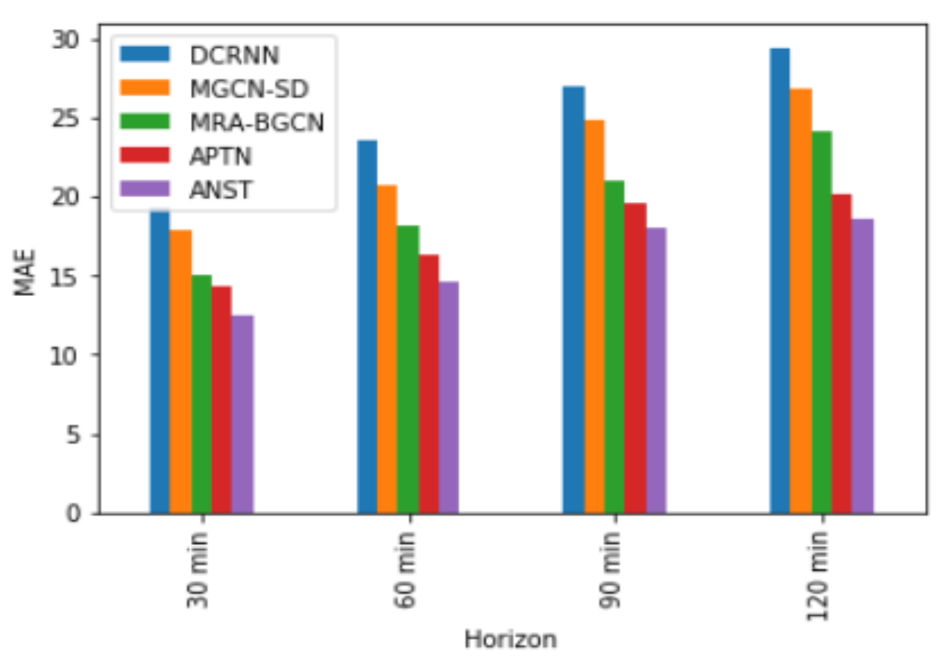
• Diffusion convolutional recurrent neural network (DCRNN): combines RNN with convolutional networks through diffusion to generate the network graph based on the distance between nodes. The spatial dependency is obtained through bidirectional random walks in the graph, and the temporal dependency is obtained through an encoder–decoder framework with sampling.
• Spatiotemporal multi-graph convolutional networks with synthetic data (MGCN-SD): deploys a generative adversarial network to generate synthetic traffic volumes along with a multi-graph convolution network to extract non-Euclidean spatial features.
• Multi-Range attentive bicomponent graph convolutional network (MRA-BGCN): deploys a node-wise graph based on the road network and an edge-wise graph for interaction patterns among edges. The multi-range attention mechanism aggregates the information from neighbouring nodes to correlate the interaction.
• Attention-based periodic-temporal neural network (APTN): models both spatial and temporal dependencies using an encoder-decoder with attention mechanisms.

The models considered are implemented using the Tensorflow framework. The dimensions of the RNN units are set up at $[16,32,64,128,N]$ and learning rates are tuned at $[0.1,0.01,0.001,0.0001]$ for 100 epochs. The model is evaluated for horizons of 30 min, 60 min, 90 min and 120 min. The overall performance is depicted in

Table 2. Comparison of different models.

Time	30 min	60 min	90 min	120 min
Model	RMSE MAE MAPE	RMSE MAE MAPE	RMSE MAE MAPE	RMSE MAE MAPE
DCRNN	24.54 19.32 15.62	27.26 23.52 16.87	31.89 26.98 18.75	35.78 29.43 20.04
MGCN-SD	21.36 17.83 12.31	24.96 20.67 15.53	29.65 24.89 16.78	33.82 26.9 17.93
MRA-BGCN	19.67 15.07 10.54	23.58 18.23 12.98	26.32 21.03 13.73	30.45 24.17 15.78
APTN	18.34 14.35 9.72	21.72 16.31 11.03	24.62 19.61 11.96	28.34 20.11 12.05
ANST	16.78 12.54 7.89	19.78 14.67 9.54	22.78 17.98 10.32	25.67 18.62 10.97

and Figure 10. It is noted that the predicted series is almost in line with the actual series on all horizons.

To be more specific, all the baseline models considered for comparison leverage a non-Euclidean structure to investigate spatial and temporal dependencies. The complexity of DCRNN has limited its performance for the considered dataset. Nonetheless, MGCN-SD is entirely based on CNN; a multi-graph convolution network is used for spatial dependency, and CNN is used to model temporal features. However, temporal dependencies are effectively modelled in MRA-BGCN, APTN and ANST with the help of RNN and its variants, thereby resulting in an improvement in performance that is clearly observed. Furthermore, attention mechanisms have been deployed in APTN and ANST to dynamically capture spatiotemporal dependencies in the region. The results show that ANST has the best performance in all forecasting horizons as region-wide traffic is considered with the inclusion of external factors such as weather, which has a key impact on traffic flow.

On the other hand, traffic prediction is challenging during peak hours. Figure 11 shows the comparison of MAE for DCRNN, MGCN-SD, MRA-BGCN, APTN and ANST during different horizons of the peak hours. Due to similarity in results, RMSE and MAPE are skipped. Furthermore, because multi-scale spatiotemporal features are fused with external factors, ANST produces smooth results even during traffic fluctuations. It can be emphasised that as the horizon increases, the performance of ANST does not deteriorate.

6. Conclusions

In this paper, multivariate prediction of spatiotemporal dependencies in non-Euclidean space with external factors is performed. The LSTM encoder adaptively chooses the spatial weights, and the LSTM decoder dynamically selects the temporal weights to form the hidden states of the model. To improve performance, all dependencies are formulated in non-Euclidean space, taking into account the similarities in the road network. External factors are combined with the output of the decoder to obtain the final predictions. ANST is assessed for future horizons and has good prediction accuracy. The model can be implemented for logistics to minimise travel costs and time.

References

1. Wang, Z.; Su, X.; Ding, Z. Long-term traffic prediction based on LSTM encoder-decoder architecture. IEEE Trans. Intell. Transp. Syst. 2021, 22, 6561–6571. [Google Scholar] [CrossRef]
2. Qu, L.; Li, W.; Li, W.; Ma, D.; Wang, Y. Daily long-term traffic flow forecasting based on a deep neural network. Expert Syst. Appl. 2019, 121, 304–312. [Google Scholar] [CrossRef]
3. Zheng, J.; Huang, M. Traffic flow forecast through time series analysis based on deep learning. IEEE Access 2020, 8, 82562–82570. [Google Scholar] [CrossRef]
4. Ghosh, B.; Basu, B.; O’Mahony, M. Multivariate short-term traffic flow forecasting using time-series analysis. IEEE Trans. Intell. Transp. Syst. 2009, 10, 246–254. [Google Scholar] [CrossRef]
5. Williams, B.M.; Hoel, L.A. Modeling and forecasting vehicular traffic flow as a seasonal ARIMA process: Theoretical basis and empirical results. J. Transp. Eng. 2003, 129, 664–672. [Google Scholar] [CrossRef] [Green Version]
6. Koesdwiady, A.; Soua, R.; Karray, F. Improving traffic flow prediction with weather information in connected cars: A deep learning approach. IEEE Trans. Veh. Technol. 2016, 65, 9508–9517. [Google Scholar] [CrossRef]
7. Voort, M.V.D.; Dougherty, M.; Watson, S. Combining Kohonen maps with ARIMA time series models to forecast traffic flow. Transp. Res. Part C Emerg. Technol. 1996, 4, 307–318. [Google Scholar] [CrossRef] [Green Version]
8. Wang, Y.; Jing, C. Spatiotemporal Graph Convolutional Network for Multi-Scale Traffic Forecasting. ISPRS Int. J. Geo-Inf. 2022, 11, 102. [Google Scholar] [CrossRef]
9. Guo, S.; Lin, Y.; Li, S.; Chen, Z.; Wan, H. Deep spatial temporal 3D convolutional neural networks for traffic data forecasting. IEEE Trans. Intell. Transp. Syst. 2019, 20, 3913–3926. [Google Scholar] [CrossRef]
10. Zang, D.; Ling, J.; Wei, Z.; Tang, K.; Cheng, J. Long-term traffic speed prediction based on multiscale spatiotemporal feature learning network. IEEE Trans. Intell. Transp. Syst. 2019, 20, 3700–3709. [Google Scholar] [CrossRef]
11. Tselentis, D.I.; Vlahogianni, E.I.; Karlaftis, M.G. Improving short-term traffic forecasts: To combine models or not to combine. IET Intell. Transp. Syst. 2015, 9, 193–201. [Google Scholar] [CrossRef]
12. Lu, S.; Zhang, Q.; Chen, G.; Seng, D. A combined method for short-term traffic flow prediction based on recurrent neural network. Alex. Eng. J. 2021, 60, 87–94. [Google Scholar] [CrossRef]
13. Chen, K.; Deng, M.; Shi, Y. A Temporal Directed Graph Convolution Network for Traffic Forecasting Using Taxi Trajectory Data. ISPRS Int. J. Geo-Inf. 2021, 10, 624. [Google Scholar] [CrossRef]
14. Hochreiter, S.; Schmidhuber, J. Long short-term memory. Neural Comput. 1997, 9, 1735–1780. [Google Scholar] [CrossRef] [PubMed]
15. Shi, X.; Qi, H.; Shen, Y.; Wu, G.; Yin, B. A Spatial–Temporal Attention Approach for Traffic Prediction. IEEE Trans. Intell. Transp. Syst. 2021, 22, 4909–4918. [Google Scholar] [CrossRef]
16. Zhu, K.; Zhang, S.; Li, J.; Zhou, D.; Dai, H.; Hu, Z. Spatiotemporal multi-graph convolutional networks with synthetic data for traffic volume forecasting. Expert Syst. Appl. 2022, 187, 115992. [Google Scholar] [CrossRef]
17. Hou, J.; Wang, Y.; Zhou, J.; Tian, Q. Prediction of hourly air temperature based on CNN–LSTM. Geomat. Nat. Hazards Risk 2022, 2022, 1962–1986. [Google Scholar] [CrossRef]
18. Chen, W.; Chen, L.; Xie, Y.; Cao, W.; Gao, Y.; Feng, X. Multi-Range Attentive Bi-component Graph Convolutional Network for Traffic Forecasting. In Proceedings of the Thirty-Fourth AAAI Conference on Artificial Intelligence (AAAI-20), New York, NY, USA, 7–12 February 2020; pp. 3529–3536. [Google Scholar]
19. Li, Y.; Yu, R.; Shahabi, C.; Liu, Y. Diffusion convolutional recurrent neural network: Data-driven traffic forecasting. Proc. Int. Conf. Mach. Learn. 2018, arXiv:1707.01926, 147–155. [Google Scholar]
20. Mingheng, Z.; Yaobao, Z.; Ganglong, H.; Gang, C. Accurate multisteps traffic flow prediction based on SVM. Math. Probl. Eng. 2013, 2013, 1–8. [Google Scholar] [CrossRef] [Green Version]
21. Sun, B.; Cheng, W.; Goswami, P.; Bai, G. Short-term traffic forecasting using self-adjusting k-nearest neighbours. IET Intell. Transp. Syst. 2018, 12, 41–48. [Google Scholar] [CrossRef] [Green Version]
22. Xie, D.F.; Fang, Z.Z.; Jia, B.; He, Z. A data-driven lane-changing model based on deep learning. Transp. Res. Part C Emerg. Technol. 2019, 106, 41–60. [Google Scholar] [CrossRef]
23. Li, L.; Qin, L.; Qu, X.; Zhang, J.; Wang, Y.; Ran, B. Day-ahead traffic flow forecasting based on a deep belief network optimized by the multi-objective particle swarm algorithm. Knowl. Based Syst. 2019, 172, 1–14. [Google Scholar] [CrossRef]
24. Kong, F.; Li, J.; Jiang, B.; Song, H. Short-term traffic Flow prediction in smart multimedia system for Internet of vehicles based on deep belief network. Future Gener. Comput. Syst. 2019, 93, 460–472. [Google Scholar] [CrossRef]
25. Zhao, L.; Zhou, Y.; Lu, H.; Fujita, H. Parallel computing method of deep belief networks and its application to traffic flow prediction. Knowl Based Syst. 2019, 163, 972–987. [Google Scholar] [CrossRef]
26. Zhang, Y.; Huang, G. Traffic Flow prediction model based on deep belief network and genetic algorithm. IET Intell. Transp. Syst. 2018, 12, 533–541. [Google Scholar] [CrossRef]
27. Sun, S.; Wu, H.; Xiang, L. City-wide traffic Flow forecasting using a deep convolutional neural network. Sensors 2020, 20, 421. [Google Scholar] [CrossRef] [Green Version]
28. Ma, X.; Dai, Z.; He, Z.; Ma, J.; Wang, Y.; Wang, Y. Learning Traffic as Images: A Deep Convolutional Neural Network for Large-Scale Transportation Network Speed Prediction. Sensors 2017, 17, 818. [Google Scholar] [CrossRef] [Green Version]
29. Sharma, B.; Kumar, S.; Tiwari, P. ANN based short-term traffic flow forecasting in undivided two lane highway. J. Big Data 2018, 5, 48. [Google Scholar] [CrossRef]
30. Hu, R.; Chiu, Y.C.; Hsieh, C.W. Crowding prediction on mass rapid transit systems using a weighted bidirectional recurrent neural network. IET Intell. Transp. Syst. 2020, 14, 196–203. [Google Scholar] [CrossRef]
31. Xiangxue, W.; Lunhui, X.; Kaixun, C. Data-driven short-term forecasting for urban road network traffic based on data processing and LSTM-RNN. Arab. J. Sci. Eng. 2019, 44, 3043–3060. [Google Scholar] [CrossRef]
32. Duives, D.; Wang, G.; Kim, J. Forecasting pedestrian movements using recurrent neural networks: An application of crowd monitoring data. Sensors 2019, 19, 382. [Google Scholar] [CrossRef] [PubMed]
33. Du, B.; Peng, H.; Wang, S.; Bhuiyan, M.Z.A.; Wang, L.; Gong, Q.; Liu, L.; Li, J. Deep irregular convolutional residual LSTM for urban traffic passenger flows prediction. IEEE Trans. Intell. Transp. Syst. 2020, 21, 972–985. [Google Scholar] [CrossRef]
34. Mou, L.; Zhao, P.; Xie, H.; Chen, Y. T-LSTM: A long short-term memory neural network enhanced by temporal information for traffic flow prediction. IEEE Access 2019, 7, 98053–98060. [Google Scholar] [CrossRef]
35. Tian, Y.; Zhang, K.; Li, J.; Lin, X.; Yang, B. LSTM-based traffic flow prediction with missing data. Neurocomputing 2018, 318, 297–305. [Google Scholar] [CrossRef]
Figure 1. Road network with sensors.
Ijgi 11 00619 g001
Figure 2. Architecture of ANST.
Ijgi 11 00619 g002
Figure 3. Spatial attention model in encoder.
Ijgi 11 00619 g003
Figure 4. Temporal attention model in decoder.
Ijgi 11 00619 g004
Figure 5. Relationship between one hot encoding and embedding vector.
Ijgi 11 00619 g005
Figure 6. Heatmap of traffic flow and weather parameters.
Ijgi 11 00619 g006
Figure 7. ANST ground truth and prediction.
Ijgi 11 00619 g007
Figure 8. Traffic flow based on weather.
Ijgi 11 00619 g008
Figure 9. Traffic flow based on holidays.
Ijgi 11 00619 g009
Figure 10. Traffic flow in different horizons.
Ijgi 11 00619 g010
Figure 11. MAE during different horizons.
Ijgi 11 00619 g011