Geographic Named Entity Recognition by Employing Natural Language Processing and an Improved BERT Model

Abstract

Toponym recognition, or the challenge of detecting place names that have a similar referent, is involved in a number of activities connected to geographical information retrieval and geographical information sciences. This research focuses on recognizing Chinese toponyms from social media communications. While broad named entity recognition methods are frequently used to locate places, their accuracy is hampered by the many linguistic abnormalities seen in social media posts, such as informal sentence constructions, name abbreviations, and misspellings. In this study, we describe a Chinese toponym identification model based on a hybrid neural network that was created with these linguistic inconsistencies in mind. Our method adds a number of improvements to a standard bidirectional recurrent neural network model to help with location detection in social media messages. We demonstrate the results of a wide-ranging evaluation of the performance of different supervised machine learning methods, which have the natural advantage of avoiding human design features. A set of controlled experiments with four test datasets (one constructed and three public datasets) demonstrates the performance of supervised machine learning that can achieve good results on the task, significantly outperforming seven baseline models.

1. Introduction

Online social media platforms, especially microblog platforms such as Wechat and Weibo, are responsive to real-world events and are useful for gathering situational information in real time [1,2,3,4]. Geographic locations are often described in these messages. For example, Weibo is widely used in disaster response and rescue, such as earthquakes, floods, fire, and terrorist attacks. The cornerstone of the aforementioned application is called geoparsing [5,6,7]. Geoparsing is a difficult natural language processing (NLP) task that aligns naturally stated things in free text spatially (written or obtained through automatic transcription) [7,8,9]. It is important to understand the distinction between geographic parsing and geocoding. The input to geographic parsing does not include any information about the places indicated in the input. In geocoding, a valid textual representation of the location (address) is the input. As a result, the geocoder needs to merely look up the supplied address’s coordinates in a gazetteer. Geocoding is difficult due to the fact that it deals with raw natural language data. In this paper, we show initial progress in creating the first geographic name parsing system for a Chinese language. To achieve this goal, the first subprocess of our approach is to identify the location of the mentioned contents; this subprocess is called entity recognition (NER) in NLP [10,11,12,13].

There are single-word place names, such as Beijing, Shanghai, Zhejiang, etc. There are also long place names composed of multiple words, such as Ejin Jinqi Saihantaolai Sumu Township (Inner Mongolia Autonomous Region); however, most of the place names are 1~5 words in length. The distribution of characters used in Chinese place names is also relatively scattered, but there are relatively concentrated features of place names within a certain range. For example, there are 3685 characters used in the gazetteer of China, and the specific frequency of use is relatively scattered. However, some of these words and their word combinations only appear in toponyms, such as “Gacha” in Inner Mongolia, while most of them are common words with strong word formation ability and often appear in nontoponymic words, such as “Suqian” in “Su” and “Qian”. Based on the above points, Chinese place names can be roughly divided into simple and complex names. Simple names refer to those with short lengths (1~5 words) and common characters, such as Beijing, Beijing Municipality, Hetao Plain, Hongyashan Reservoir, etc. Complex names refer to those with long lengths (more than five words) or with characters and words that are more remote. Therefore, it is technically difficult to identify Chinese place names accurately, and it has become an important research direction in the field of geographic information.

The existing methods for recognizing geographical names can be divided into three types of methods: rule-based methods, statistical methods, and machine learning methods [14,15]. Rule-based methods refer to the manual summarization of various word formations and syntactic rules and recognition by rule matching methods. This method is more intuitive, easy to understand and extend, and works better and faster for small-scale corpus testing. However, the design of rules relies on professional language knowledge and domain knowledge, is time-consuming to compile, is difficult to cover comprehensively, and has poor portability and robustness. The statistical-based approach does not require specialized language knowledge, is more robust and flexible than the rule-based approach, and is highly portable, but the system does not express language determinism well and requires a large-scale, more comprehensive manually annotated training corpus. With the accumulation of big data and the continuous enhancement of computer performance, deep-learning-based place-name-extraction methods have been developed rapidly. Deep learning models are application-friendly and robust and can automatically learn and extract key features from text, achieving remarkable results in Chinese place-name recognition. The most commonly used model is bidirectional long short-term memory (LSTM), which is based on the evolution of recurrent neural networks (RNNs) and overcomes the shortcomings of RNNs in long-dependent sentences. The two-way LSTM uses two LSTM hidden layers with opposite directions to further solve the problem that sequence tagging can only use information from above and not below. In the current research on Chinese place-name recognition, the main problem focuses on the recognition of complex Chinese place names. Since the length of complex place names is usually long and the use of words and word collocation is relatively small, the above models often have difficulty determining the boundaries of place names.

In this paper, we propose a hybrid neural network model for Chinese place-name recognition based on a bidirectional encoder of the lite bidirectional encoder representations from transformers (ALBERTs) model for word vector extraction to improve the text vector representation ability and effectively identify irregular place names and place-name abbreviations. The bidirectional long- and short-term memory (BiLSTM) neural network layer captures the semantic information in both directions in the sentence to better determine the entity boundaries. The global optimal token sequence is obtained by the conditional random field (CRF) layer.

The main contributions of this research are listed as follows:

(1) TPCNER, a large self-annotated corpus of geographic domains with seven categories and 64,063 labeled samples, was gathered and built. This corpus has more entity categories and larger sample sizes than the preceding corpora. The efficiency of the TPCNER highlighted in this study was further demonstrated by the assessment experimental findings in Section 5.4.

(2) A novel Chinese NER (CNER) model for the geographic domain via the improved ALBERT pretraining model and BiLSTM–CRF was proposed. By learning word-level feature representation through the ALBERT layer and extracting text contextual semantic features through the BiLSTM layer, the CRF layer obtains the global optimal token sequence and finally improves the overall performance of the proposed model.

(3) The performance of ALBERT–BiLSTM–CRF was evaluated by using a range of standard models on TPCNER, MSRA, RenMinRiBao, and Boson. Furthermore, several specific details were studied and debated, such as the efficacy of BiLSTM and the use of the CRF mechanism. Through thorough comparisons with other advanced models, comprehensive experimental findings on domain-specific and generic datasets confirmed the proposed model’s effective performance.

The rest of the paper is organized as follows: The current work on named-entity recognition is described in Section 2. The processing of corpus creation is described in Section 3. The recommended procedure for identifying geographic entities is presented and described in Section 4. Section 5 contains the experimental data and results. The conclusion and recommendations for further study are presented in Section 6.

2. Related Work

Toponym information contains spatial location information, so toponym recognition can be applied to emergency-disaster reduction, public-opinion monitoring, urban planning, and other fields [16,17,18]. For example, information such as place names and natural disasters occurring there can be extracted from social media messages released by the public, such as Twitter. Social media messages can also assist in the monitoring and management of public opinion. Managers can identify social public-security events from webpages and social media texts and extract key spatial location information, realize the monitoring and early warning of social public security incidents, and improve the efficiency of social and public security time disposal. To protect public privacy, social media will selectively hide the specific user location obtained in real time, which makes the extraction of geographic location information more complicated. In June 2019, Twitter officially removed the precise geotagging feature. This change may reduce the geographic information contained in tweets, complicate location judgment, and make the task of recognizing and geolocating locations from tweet content more urgent when dealing with emergencies [15]. We mainly identify the long text toponymic information in more detail to make its characteristics more obvious and facilitate the development of subsequent tasks.

The recognition methods of Chinese toponyms are mainly divided into three types, namely dictionary and rule-based methods, statistical-based machine learning methods, and deep learning methods [19,20,21]. The rule-based method mainly carries out place-name matching and recognition by manually summarizing various word-formation rules (the defects of this method have been summarized in Section 1), which can be combined with the current popular deep learning methods to supplement professional vocabulary and improve the robustness of the training model. The number of toponyms will increase at an extremely fast rate with the development of the region, and frequently the same location is represented by multiple toponyms. Therefore, the construction of a definitive gazetteer cannot be achieved, and automatic place-name recognition is still worth studying.

The method based on statistics is more flexible than the rule method, which transforms place-name recognition into a serialization annotation problem, but this method depends on the selection of feature templates and has poor generalization ability. Common machine learning algorithms include the hidden Markov model (HMM), maximum entropy Markov model (MEMM), and CRF model. Among them, the CRF model can implement effective feature-selection and feature-induction algorithms for sequence-labeling tasks. That is, users can evaluate the effect of automatically generated features on data abstraction. Therefore, combining a CRF model with subsequent large-scale pretraining models, such as the BERT–CRF model, can achieve excellent sequence labeling results, thus providing ideas for more accurate place-name recognition.

The named-entity identification approach based on neural networks is extensively utilized in text information extraction in numerous sectors, thanks to the rapid growth of deep learning. Different from traditional machine learning algorithms, the model trained by a deep neural network has the characteristics of end-to-end data input and output. It makes the model training process more capable of reducing artificial interference to directly complete specific tasks according to the original data input, and there is no need to manually set data characteristics [22]. The RNN is especially good at processing sequence data. The evolved LSTM, BiLSTM, and bidirectional gated recurrent unit (BiGRU) networks often combine the CRF layer to realize the task of named entity recognition. The more common BiLSTM–CRF model, which combines the advantages of BiLSTM and CRF, not only can retain the context information to process long text but also fully use sentence-level tag information thanks to a CRF layer. Similarly, the BiGRU–CRF model is widely used.

In recent years, large-scale pretraining models have rapidly become the preferred method of natural language processing due to their outstanding performance. On this basis, downstream task processing can make the recognition results of the hybrid model more accurate [23,24]. Common pretraining models include the generative pretrained transformer (GPT), BERT, enhanced representation through knowledge integration (ERNIE), etc. The current popular BERT model works from the encoder of the bidirectional transformer model [25,26]. We choose the BERT-wwm model as the pretraining model, which is trained by the Research Center for Social Computing and Information Retrieval and iFLYTEK AI Research in China. It is an open-source Chinese pretraining language model, using whole-word masking technology, which can better realize the task of Chinese place-name recognition. On the basis of BERT-wwm, BERT-wwm-ext expands the pretraining dataset and increases the number of training iterations during model training.

Toponym recognition is a subtask of named entity recognition, which belongs to the information extraction task. We want to extract place-name information from long text data, but the model trained by the general corpus is still lacking in the accuracy and granularity of toponym recognition. In response to the above problems, we used a Chinese corpus containing only toponym annotations and designed a hybrid neural network to train the model to obtain a model that performs better in the task of Chinese toponym recognition. This model improves upon the general effect and low granularity of the traditional named-entity recognition model in toponym recognition.

3. Corpus Preparation and Annotation

To address the limited Chinese NER corpus, a new corpus, TPCNER, was collected and constructed. The dataset was further extended with entity categories based on earlier studies and eventually contained 7 entity categories and 64,063 annotated samples.

3.1. NER Tag Sets

Named entities in the geographic domain, such as organizations, water systems, and landforms, are very different from those in the general domain. Geographic entities require a large amount of domain-specific knowledge, thus making annotation difficult to a certain extent. In this paper, based on the existing research [24], the entity categories are further divided into more granular entities, such as residential land and facilities, landforms, and water systems. Some categories were also considered, such as transportation, pipelines, boundaries, and political areas with other regions. Finally, as indicated in

Table 1. Details of entity categories in TPCNER.

ID	Entity Tags	Abbreviation	Description	Example
1	Water System	WAT	A manmade building or natural structure associated with water in nature.	Tongji Canal, Huaihe River Basin
2	Residential land and facilities	RLF	A place where human beings live or engage in productive life.	Shaanxi Kiln
3	Transportation	TRA	Human-built buildings related to transportation.	Longxia Railway
4	Pipelines	PIP	Pipelines laid by humans.	Natural gas pipeline
5	Boundaries, Regions, and Other Areas	BRO	The corresponding boundaries that humans have drawn on the land to facilitate management.	Hubei Province
6	Landforms	LAN	Includes natural and artificial landforms.	Himalayas
7	Organization	ORG	Includes the names of relevant organizations.	Wuhan Zhongdi Digital Technology Co.

, seven fine-grained groups emerge. To guarantee the integrity of the CNER categories, we predefine the category “others” in this work to characterize some conceptual and uncertain entities for later growth. Furthermore, this article exclusively considers entity types that are relevant to the geographic domain (e.g., toponym and organization), rather than generic entities such as individuals (e.g., personal name). In the future, the corpus will be released as well.

Table 2. Details of entity categories in Boson.

ID	Entity Tags	Abbreviation	Description	Example
1	Location	LOC	A spatial distribution, location, or place occupied.	China
2	Org_name	ORG	Includes the names of relevant organizations.	Wuhan Zhongdi Digital Technology Co.

,

Table 3. Details of entity categories in MSRA.

ID	Entity Tags	Abbreviation	Description	Example
1	NS	NS	A spatial distribution, location, or place occupied.	Yufeng Mountain
2	NT	NT	Includes the names of relevant organizations.	China University of Geosciences

and

Table 4. Details of entity categories in RenMinRiBao.

ID	Entity Tags	Abbreviation	Description	Example
1	NS	NS	A spatial distribution, location, or place occupied.	Hubei
2	NT	NT	Includes the names of relevant organizations.	China University of Geosciences

show the details of Boson, MSRA, and RenMinRiBao.

3.2. Corpus Collection and Annotation

In this paper, a large-scale annotated corpus, TPCNER, is established with the Baidu Encyclopedia and the Chinese Encyclopedia of Chinese Geography as source data (approximately 2 million words) and with reference to the geographically named entity annotation system designed in this paper.

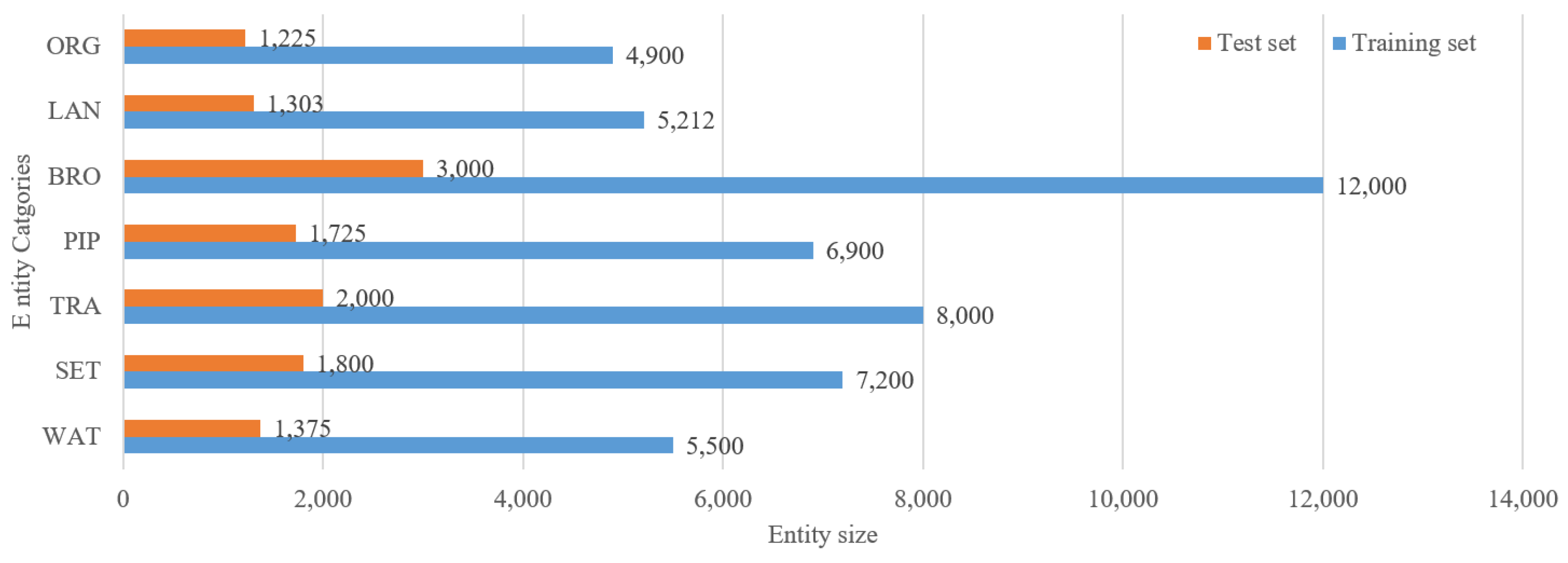
To ensure consistency and accuracy, the work in this paper is presented in two main areas. First, a new TPCNER annotation tool, ChineseNERAnno, was developed (see Figure 1). The complete process of this tool is depicted in Figure 1. The suggested technique employs a lexicon of terms linked to the geographic domain for automated annotation, which helps to ensure entity consistency. Second, new entities can be dynamically extended into the dictionary, thus reducing the manual annotation time and increasing the annotation speed. A new TPCNER corpus was finally constructed, consisting of 7 categories, 650,725 entities, and 64,063 samples preprocessed and annotated. This procedure took three months to complete under the supervision of domain experts.

Table 5. Some samples of TPCNER.

Sentence(en):	Anji County is a county in Huzhou City, Zhejiang Province, a famous bamboo producing area in China and one of the key forestry counties in Zhejiang Province.
Label(en):	Anji County; Zhejiang Province; Huzhou City; China; Zhejiang Province
Sentence(en):	The Bailong River is a tributary of the upper reaches of the Jialing River in the Yangtze River system, and is a geographically important dividing line in China, along with the Qinling and Huai Rivers.
Label(en):	Bailong River; Yangtze River; Jialing River; Qinling River; Huai River; China

shows certain TPCNER examples in further detail. Figure 2 shows data on the statistical distribution of individual entities in TPCNER, demonstrating that the training set’s distribution is similar to the validation set’s distribution. The logic and utility of the corpus designated in this work are also argued in Section 5.4.

3.3. Analysis of Corpus Features

Geographic entity names are the most important distinction between geographic entities and in the field of geographic information (see

Table 6. Comparative information between TPCNER and other datasets.

Datasets	Examples	Classes	Size	Entity Size	Max Length	Min Length	Avg Length
Boson	Obama[person_name] also welcomed Cameron[person_name] using a number of authentic British[location] vernaculars,	6	1.78 M	3417	36	1	18.5
MSRA	the scope of the survey involved the Forbidden City[location], the Museum of History[location], the Institute of Ancient Research[organization_name], the Peking University and Tsinghua Library[location], the Beitu[location], the Japanese archives and more than twenty others.	3	10.4 M	80,884	40	1	20.5
RenMinRiBao	New Year Concert in Beijing[location]	3	10.1 M	12,718	35	1	18
TPCNER	The sample examples are listed in Table 2.	7	7.32 M	64,063	18	2	10

). Entity names with location information, mainly composed of basic geographic information elements, can be seen with ambiguity and diversity. In this paper, we analyze the descriptive features of geographic entities in texts by studying relevant national standards and the literature. We then integrate geographically named entity categories and descriptive features by manual collation and data fusion with national standards as the benchmark. The distribution for each category in TPCNER is shown in Figure 2.

The descriptions of geographic entity names in Chinese texts are characterized by vagueness, uncertainty, and diversity. In this paper, we analyze the descriptive features of geographic entity names in texts. The five main descriptive features are summarized as follows:

(1) The names of geographic entities are diverse, with free and scattered words or phrases, but with relatively concentrated coverage, for example, the name of the community “Daijiashanzhuang”, within which there are “Daijiashanzhuang Phase 1” and “Daijiashanzhuang Phase 2”.

(2) The names of geographical entities have a certain pattern, often ending with characteristic words, such as “province, road, mountain”, for example, “Hubei Province” and “Luma Road, Hongshan District, Hubei Province”.

(3) The names of geographical entities are often followed by location words; for example, “Huangshan” is a place name, and “Huangshan North” is a complete geographical naming entity.

(4) Most of the names of geographical entities are in the form of nouns, but sometimes they are used as modifiers to modify other entities, such as “Bagong Mountain Tofu”.

(5) The names of geographical entities are named and unnamed; that is, some geographical entities do not have specific names, and their spatial locations need to be determined through the contextual relationship. For example, the “swimming pool” in the “swimming pool in the west area of the university” is the name of a geographical entity, but its spatial location needs to be determined by the previous information.

4. The Hybrid Deep Learning Model

4.1. Overall Framework and Workflow of the Model

In this paper, we propose a hybrid neural network model for Chinese place-name recognition. The overall structure of the model is shown in Figure 3, and the whole model is divided into five parts: the input layer, ALBERT layer, BiLSTM layer, CRF layer, and output layer.

We present our model from bottom to top, characterizing the layers of the neural network. The input layer contains the individual words of a message which are used as the input to the model.

The next layer represents each word as vectors, using a pretraining approach. It uses pretrained word embeddings to represent the words in the input sequence. In particular, we use ALBERT, which captures the different semantics of a word under varied contexts. Note that the pretrained word embeddings capture the semantics of words based on their typical usage contexts and therefore provide static representations of words; by contrast, ALBERT provides a dynamic representation for a word by modeling the particular sentence within which the word is used. This layer captures four different aspects of a word, and their representation vectors are concatenated together into a large vector to represent each input word. These vectors are then used as the input to next layer, which is a BiLSTM layer consisting of two layers of LSTM cells: one forward layer capturing information before the target word and one backward layer capturing information after the target word.

The BiLSTM layer combines the outputs of the two LSTM layers and feeds the combined output into a fully connected layer. Then the next layer is a CRF layer, which takes the output from the fully connected layer and performs sequence labeling. The CRF layer uses the standard BIEO model from NER research to label each word but focuses on locations. Thus, a word is annotated as either “B–L” (the beginning of a location phrase), “I–L” (inside a location phrase), “E–L” (end a location phrase), or “O” (outside a location phrase).

The workflow of the model is as follows:

(1) First, the dataset is composed of text X (X₁, X₂, …, X_n), which is input to the ALBERT layer, where X_i denotes the i-th word in the input text.

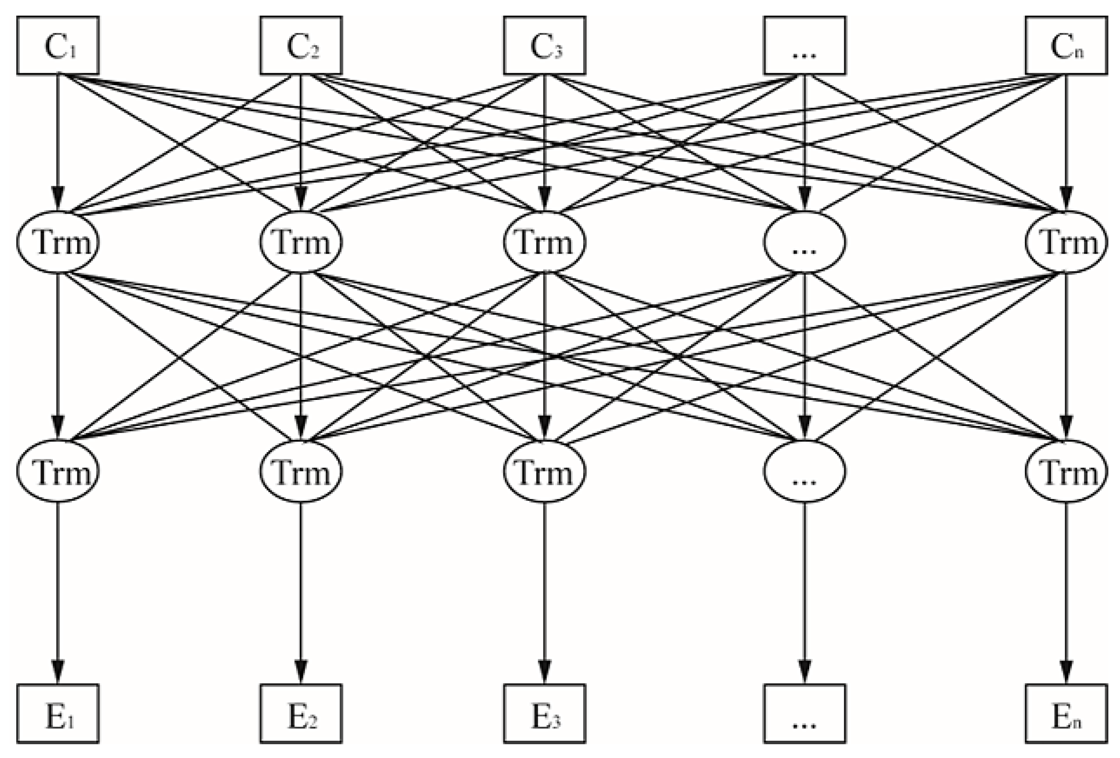
(2) The input text data are serialized in the ALBERT layer, and the model generates feature vectors, C_i, based on each word, X_i, in the text to enhance the text vector representation and transforms C_i into word vectors, E = (E₁, E₂, …, E_n), with location features based on Transformer (Trm) in the word vector representation layer of ALBERT.

(3) Using E_i as the input of each time step of the bidirectional LSTM layer and performing feature calculation, the forward LSTM F = (F₁, F₂, …, F_n) and the reverse LSTM B = (B₁, B₂, …, B_n) of the BiLSTM layer are used to extract the contextual features and generate the feature matrix, H = (H₁, H₂, …, H_n), by position splicing to capture the semantic information in both directions in the sentence.

(4) Consider the transfer features between annotations in the CRF layer, obtain the dependencies between adjacent labels, and output the corresponding labels Y (Y₁, Y₂, …, Y_n) to obtain the final annotation results.

4.2. BERT and ALBERT Pretraining Models

The pretraining model provides a better initialization parameter for the neural network, accelerates the convergence of the neural network, and provides better generalization ability on the target task. The development of pretraining models is divided into two stages: shallow word embedding and deep coding. The shallow word embedding models mainly use the current word and previous word information for training; they only consider the local information of the text and fail to effectively use the overall information of the text [22,27]. BERT uses a bidirectional transformer network structure with stronger epistemic capability to train the corpus and achieve a deep bidirectional representation for pretraining [25]. The BERT model’s “masked language model” (MLM) can fuse the left and right contexts of the current word. BERT has achieved remarkable results in tasks such as named-entity recognition [28], text classification, machine translation [29], etc. The next sentence prediction (NSP) captures sentence-level representations and obtains semantically rich, high-quality feature representation vectors.

However, the BERT model contains hundreds of millions of parameters, and the model training is easily limited by hardware memory. The ALBERT model is a lightweight pretrained language model that is based on the BERT model [30]. The BERT model uses a bidirectional transformer encoder to obtain the feature representation of text, and its model structure is shown in Figure 4. ALBERT has only 10% of the number of parameters of the original BERT model but retains the accuracy of the BERT model.

The transformer structure of the BERT model is composed of an encoder and decoder. The encoder part mainly consists of six identical layers, and each layer consists of two sub-layers, the multi-head self-attention mechanism and the fully connected feed-forward network, respectively. Since each sub-layer is added with residual connection and normalization, the output of the sub-layer can be represented as shown in the following equation:

$$sub\_layer\_output=LayerNorm\left(x+\left(SubLayer\left(x\right)\right)\right)$$

(1)

The multi-head self-attention mechanism projects the three matrices, namely Q, V, and K, by h different linear transformations and finally splices the different attention results. The main calculation equation is shown below:

$$attention\_output=Attention\left(Q,K,V\right)$$

(2)

$$MultiHead=Concat\left(hea{d}_1,\dots ,hea{d}_h\right)W^O$$

(3)

$$hea{d}_i=Attention\left(Q{W}_i{}^Q,K{W}_i{}^K,V{W}_i{}^V\right)$$

(4)

For the decoder part, the basic structure is similar to the encoder part, but with the addition of a sub-layer of attention.

ALBERT uses two methods to reduce the number of parameters: (i) factorized embedding parameterization, which separates the size of the hidden layer from the size of the lexical embedding matrix by decomposing the huge lexical embedding matrix into two smaller matrices; and (ii) cross-layer parameter sharing, which significantly reduces the number of parameters of the model by sharing the parameters of the neural layer of the model without significantly affecting its performance.

In the figure, C = (C₁, C₂, …, C_n) indicates that each character in the sequence is trained by a multilayer bidirectional transformer (Trm) encoder to finally obtain the feature vector of the text, denoted as E = (E₁, E₂, …, E_n). After the input text is first processed by word embedding, the positional information encoding (positional encoding) of each word in that sentence is added. The model learns more text features by combining multiple self-attentive layers to form multi-head attention. The output of the multi-head attention-based layer is passed through the Add&Nom layer, where “Add” means adding the input and output of the multi-head attention layer, and “Norm” means normalization. The result, after passing through the Add&Nom layer, is passed to the feed-forward neural layer (Feed Forward) and outputted by the Add&Norm layer.

The ALBERT used in this paper has several design features that enhance its performance on the task of toponym recognition from social media messages. First, our presented ALBERT uses the pretrained word embeddings that are specifically derived from social media messages. We performed the following steps on the basis of the collected text data: (1) cleaning the data—we removed the messy codes and incomplete sentences to ensure that the sentences were smooth; (2) cutting the sentences—we added [CLS], [SEP], [MASK], etc., to each text item to obtain 25.6 GB of training data; and (3) training corpus—we trained on 3090 GPU for 4 days, with the epoch set to 100,000 and learning rate set to 5 × 10⁻⁵.

We used the GloVe word embeddings (the number of tokens is 54,238, and the dictionary size is 399 KB) that were trained on 2 billion texts, with 11 billion tokens and 1.8 million vocabulary items collected from Baidu Encyclopedia, Weibo, WeChat, etc. These word embeddings, specifically trained on a large social-media-messages corpus, include many vernacular words and unregistered words used by people in social media messages. Previous geoparsing and NER models typically use word embeddings trained on well-formatted text, such as news articles, and many vernacular words are not covered by those embeddings. When that happens, an embedding for a generic unknown token is usually used to represent this vernacular word and, as a result, the actual semantics of the word are lost. Second, compared with the basic BiLSTM–CRF model, our presented model adds an ALBERT layer to capture the dynamic and contextualized semantics of words.

4.3. BiLSTM Layer

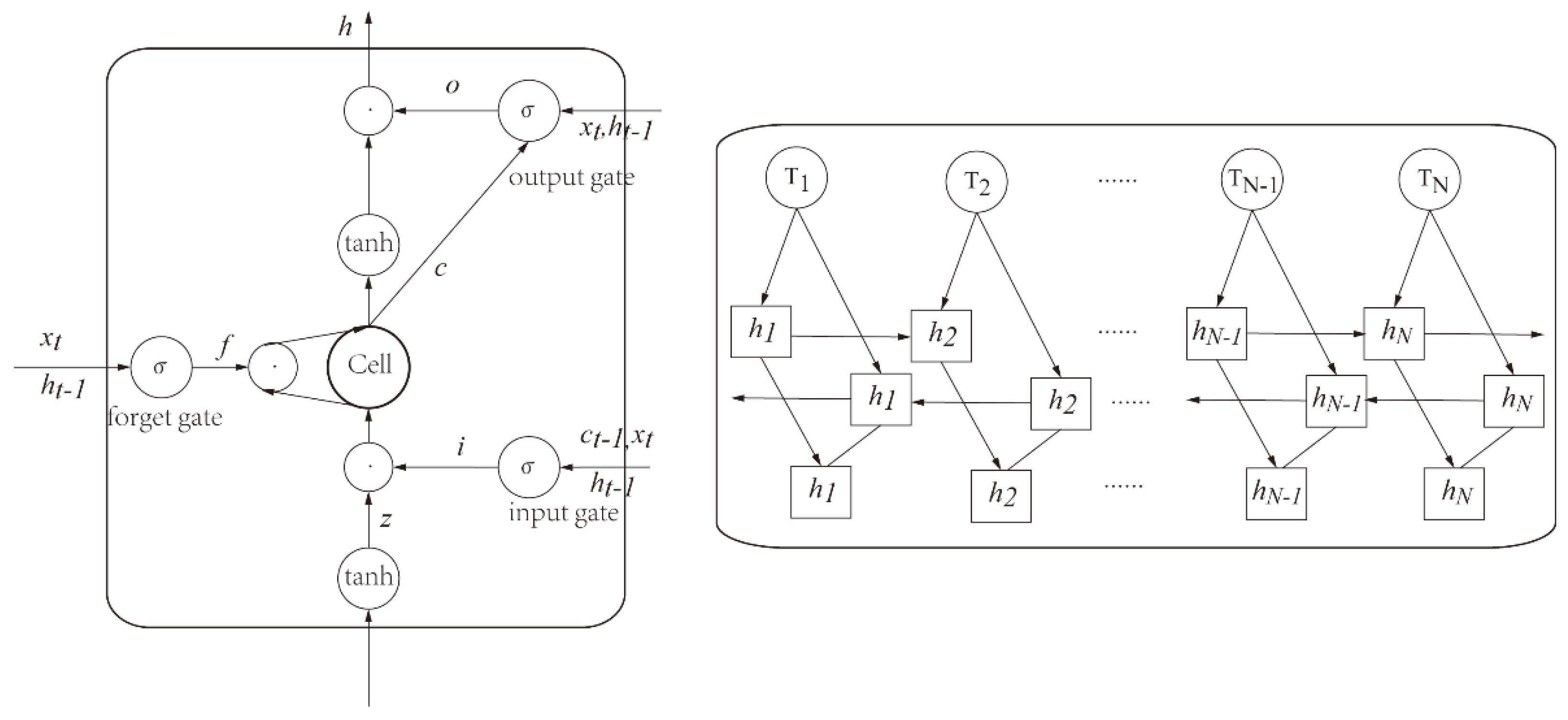
Recurrent neural networks are more suitable for sequence annotation tasks due to their ability to remember the historical information of text sequences. An LSTM model was proposed in the literature [31,32,33,34] that incorporates specially designed memory units in the hidden layer compared to RNNs and can better solve the problem of gradient explosion or gradient disappearance that RNNs tend to have as the sequence length increases. The neuron structure of the LSTM model is shown in Figure 5.

The LSTM network consists of three gate structures and one state unit; these gate structures include input gates, oblivion gates, and output gates. The input gate determines how much of the input to the network is saved to the cell state at the current moment. The forgetting gate selectively discards certain information. The output gate determines the final output value based on the cell state. The long-term dependency problem of recurrent neural networks can be better solved by the three-gate structure to maintain and update the state for long-term memory function. A typical LSTM network structure can be represented formally in Equations (5)–(10):

$$i_t=\sigma \left(W_i\cdot \left[h_{t-1},x_t\right]+b_i\right)$$

(5)

$$f_t=\sigma \left(W_f\cdot \left[h_{t-1},x_t\right]+b_f\right)$$

(6)

$$o_t=\sigma \left(W_o\cdot \left[h_{t-1},x_t\right]+b_o\right)$$

(7)

$${\tilde{C}}_t=\tan h\left(W_c\cdot \left[h_{t-1},x_t\right]+b_C\right)$$

(8)

$$C_t=f_t\otimes C_{t-1}+i_t\otimes {\tilde{C}}_t$$

(9)

$$h_t=o_t\otimes tan h\left(C_t\right)$$

(10)

where x_t represents the input word at moment t; i_t represents the memory gate; f_t represents the forget gate; o_t represents the output gate; C_t represents the cell state; ${\tilde{C}}_t$ represents the temporary cell state; h_t represents the hidden state output at each time step; h_t−1 represents the hidden state at the previous moment; C_t−1 represents the cell state at the previous moment; W_i, W_f, W_o, and W_c represent the weight matrix at the current state; and b_i, b_f, b_o, and b_C denote the offset of the current state, respectively.

4.4. CRF Layer

The conditional random field model is a discriminative probabilistic model [34]. The conditional random field model combines the advantages of the HMM and maximum entropy model (MEM). It addresses the strict independence assumption condition of the hidden Markov model, avoids the disadvantages of the local optimum and labeling bias problem of the maximum entropy model, is suitable for the labeling of sequence data CRF, considers the sequential problem among labels, and obtains the global optimal labeling sequence through the relationship of adjacent labels, adding constraints to the final predicted labels. For example, a tag starting with “B” is not followed by an “O” class tag, and a tag starting with “E” cannot be sequentially connected with tag “I” sequence. Assuming that the model input, x = (x₁, x₂, …, x_n), has a sequence of tags, y = (y₁, y₂, …, y_n), the score vector of the sentence can be calculated by Equation (7):

$$score\left(x,y\right)={\displaystyle \sum _{j=1}^n}{P}_{i,y_i}+{\displaystyle \sum _{j=0}^n}{A}_{y_i,y_{i+1}}$$

(11)

where P_i,yi is the probability of the y_i label of the character, and A is the transfer probability matrix. The CRF score vector is normalized and trained by using the log-likelihood function as the loss function, as shown in Equation (8):

$$\lg (P(y\mid x))=score\left(x,y\right)-\lg ({\displaystyle \sum _{y^{\prime }\in Y_x}}\exp \left(score\left(x,y^{\prime }\right)\right))$$

(12)

In the prediction phase, the network model is labeled by using the Viterbi algorithm to obtain the optimal sequence, as shown in Equation (9):

$$\begin{gathered} y^{*}=\arg \max score\left(x,y^{\prime }\right) \\ {\displaystyle y^{\prime }\in Y_x} \end{gathered}$$

(13)

5. Results and Discussion

On several datasets, the proposed model’s performance was compared to that of other deep learning models. Many parts of the experimental data were evaluated and debated. TensorFlow was used to implement the models on a single NVIDIA GeForce RTX 3090 GPU. Due to the nature of replication, these results may change somewhat from the originals.

5.1. Dataset, Evaluation Metrics, and Hyperparameters

Performance measures: The experiment’s measurements were precision (P), recall (R), and the F1-score (F1). Precision measures the percentage of correctly identified toponyms (true positives, TPs) among all the toponyms recognized by a model, which include both true positives and false positives (FPs). Recall measures the percentage of correctly identified toponyms among all the toponyms that are annotated as ground truth, which include true positives and false negatives (FNs). The F-score is the harmonic mean of precision and recall [35]. It is high when both precision and recall are fairly high, and it is low if either of the two is low [36].

Training process: In this study, we trained word embeddings on a Wikipedia corpus by using the word2vec tool in advance, and we concatenated consecutive words to represent an entity when the entity had multiple words. More importantly, the word embeddings obtained by word2vec were used as the initial representation of words. We treated them as parameters and modified them in the training process, which can provide a better representation of words.

Testing methodology: We used 10-fold cross-validation for testing and reported the average score of 10 independent runs. This resulted in a total of 100 different splits into training/testing subsets.

Each Chinese character was treated as a token, and TPCNER was coded by using the BIO tagging technique. To avoid overfitting, the dropout was adjusted to 0.5. Due to the likelihood of contextual reliance between neighboring phrases, the maximum length of the samples was considered to be the maximum training length, and we noted that dividing the samples might result in semantic loss. To assist the convergence of all models, the number of epochs was fixed to 100. At a ratio of 8:2, all datasets were randomly partitioned into training and validation sets.

Table 7. Comparative information between TPCNER and other datasets.

Dataset	Classes	Size	Entity Size	Max Length	Min Length	Avg Length
Boson	6	1827 kb	3417	36	1	19
MSRA	3	7.92 MB	19,871	47	1	24
RenMinRiBao	3	10,421 kb	12,718	35	1	18
TPCNER	7	7.32 MB	64,063	18	2	10

compares TPCNER to other datasets and provides comparative data.

Table 8. ALBERT model parameter.

No.	Parameter	Value
1	Hidden size	768
2	Embedding size	128
3	Max position embeddings	512
4	No. of attention heads	12
5	No. of hidden layers	12

lists the remaining hyperparameters.

5.2. Baselines

To evaluate the effect of our presented model, we empirically compared our method (ALBERT–BiLSTM–CRF) with six strong baselines (DBN, DM_NLP, NeuroTPR, CheseBERTTP, ChineseTR, and GazPNE2). In order to guarantee a relatively fair comparison, for these baselines, we employed their publicly released source codes and followed the parameter settings reported in their papers.

• DBN is an adapted toponym recognition approach based on deep belief network (DBN) by exploring two key issues: word representation and model interpretation proposed by [37].
• DM_NLP is a general model based on BiLSTM–CRF, proposed by [38].
• NeuroTPR is a Neuro-net ToPonym Recognition model designed specifically with these linguistic irregularities in mind, proposed by [39].
• ChineseBERTTP is a deep neural network named BERT–BiLSTM–CRF, which extends a basic bidirectional recurrent neural network model (BiLSTM) with the pretraining bidirectional encoder representation from transformers (BERT) representation to handle the toponym recognition task in Chinese text [40].
• ChineseTR is a weakly supervised Chinese toponym recognition architecture that leverages a training dataset creator that generates training datasets automatically based on word collections and associated word frequencies from various texts and an extension recognizer that employs a basic bidirectional recurrent neural network based on particular features designed for toponym recognition proposed by [41].
• GazPNE2 is a general approach for extracting place names from tweets, named GazPNE2. It combines global gazetteers (i.e., OpenStreetMap and GeoNames), deep learning, and pretrained transformer models (i.e., BERT and BERTweet), which require no manually annotated data [42].

5.3. Experiments on TPCNER

In this study, the HMM, CRF, BiLSTM–CRF, IDCNN–CRF, IDCNN–CRF2, BiLSTM–Attention–CRF, BERT–BiLSTM–CRF, BERT–BiGRU–CRF, ALBERT–BiLSTM, ALBERT_old–BiLSTM–CRF (original ALBERT), and ALBERT_ours–BiLSTM–CRF (our presented ALBERT) models were used to test the TPCNER dataset, and the performance of named-entity recognition was evaluated by four indices: accuracy, precision, recall, and F1-score. The experimental results are shown in

Table 9. Results of different models on TPCNER.

Model	Accuracy	Precision	Recall	F1-Score
HMM	80.9% − 0.16%	80.4%	81.5%	80.7%
CRF	83.8% + 0.03%	83.8%	84.1%	84%
BiLSTM–CRF	86.1% − 0.02%	97.9%	76.6%	86.0%
IDCNN–CRF	86.5% + 0.11%	97.9%	77.1%	86.2%
IDCNN–CRF2	88.2% + 0.25%	98.0%	79.5%	87.8%
BiLSTM–Attention–CRF	89.1% − 0.09%	97.5%	72.8%	83.4%
BERT–BiLSTM–CRF	91.1% − 0.08%	92.8%	91.5%	92.1%
BERT–BiGRU–CRF	93.4% − 0.28%	93.9%	94.9%	94.4%
ALBERTold–BiLSTM	88.1% + 0.12%	91.2%	90.7%	90.9%
ALBERTours–BiLSTM	92.7% + 0.17%	94.1%	94.5%	94.3%
ALBERTold–BiLSTM–CRF	90.5% + 0.03%	92.5%	94.4%	93.4%
ALBERTours–BiLSTM–CRF	97.8% + 0.07%	96.1%	96.2%	96.1%

. The following results can be observed:

(1) Compared with the non-neural-network models (i.e., HMM and CRF), neural network models improve the performance significantly, as the performance of the former deteriorates quickly, while the latter can maintain a reasonable performance. This is due to the fact that most of the features used in non-neural-network models come from human-designed features, which suffer from accumulated errors that may lead to performance degradation.

(2) We can see that these eleven models achieved a good performance on the TPCNER dataset, and their accuracy, precision, recall, and F1-scores frequently exceeded 80%. Among them, the ALBERT_ours–BiLSTM–CRF model has the best test effect, and its accuracy, precision, recall, and F1-score are 97.8%, 96.1%, 96.2%, and 96.1%, respectively. Compared with the other nine models, this model has a better named-entity recognition effect on the TPCNER dataset. In particular, our re-trained ALBERT model improved by 7.8% compared to the original ALBERT model.

(3) In addition, IDCNN–CRF2 achieved a better performance than IDCNN–CRF, and IDCNN–CRF and BiLSTM–CRF obtained almost the same performance; both of these results indicate that IDCNN utilizes dilated convolution to speed up training and does not enhance sequence features to improve performance.

We continued our experiments by comparing ALBERT–BiLSTM–CRF with six deep-learning-based models. The performance of these models on the TPCNER dataset is reported in

Table 10. Comparison with previous works on TPCNER.

Model	Precision	Recall	F1-Score
DBN	0.781	0.774	0.78
DM_NLP	0.838	0.841	0.84
NeuroTPR	0.871	0.872	0.87
ChineseBERTTP	0.89	0.894	0.89
ChineseTR	0.85	0.86	0.85
GazPNE2	0.835	0.849	0.84
ALBERTours–BiLSTM–CRF	0.961	0.962	0.961

. We made the following observations:

(1) ALBERT–BiLSTM–CRF yields the highest precision with the same recall. Moreover, ALBERT–BiLSTM–CRF obtains a constant and substantial improvement over ChineseBERTTP, which currently has the best results reported on this dataset, with higher precision for the same recall. We believe that the combination of specially designed ALBERT features constitutes more significant features and promotes the extractor to make accurate predictions.

(2) Compared with the basic BiLSTM–CRF model, ALBERT–BiLSTM–CRF performs better in all three metrics, thus demonstrating the value of our improved designs, including the specially designed ALBERT layers. Compared with DM_NLP and NeuroTPR, ALBERT–BiLSTM–CRF shows higher precision, a higher F1-score, and similar recall.

As expected from Table 6 and Table 7, for all datasets, ALBERT_ours–BiLSTM–CRF achieves the best F1-score, i.e., 96.1%. Compared with two weakly supervised deep-learning models (NeuroTPR and GazPNE2), our presented model performs better in all three metrics, thus demonstrating the value of our improved design, which contains a fine-tuned ALBERT. The reason is that Chinese texts often include a considerable number of location names, which may not be covered by the basic BERT, including many vernacular words (e.g., “Mengliang Mountains” and “Plateau”) and abbreviations (e.g., “Dida” and “CUG”) applied by people. When this happens, generic unknown token embedding is usually used to represent the vernacular word, and the actual semantics of the word is lost.

5.4. Experiments on the Public Dataset

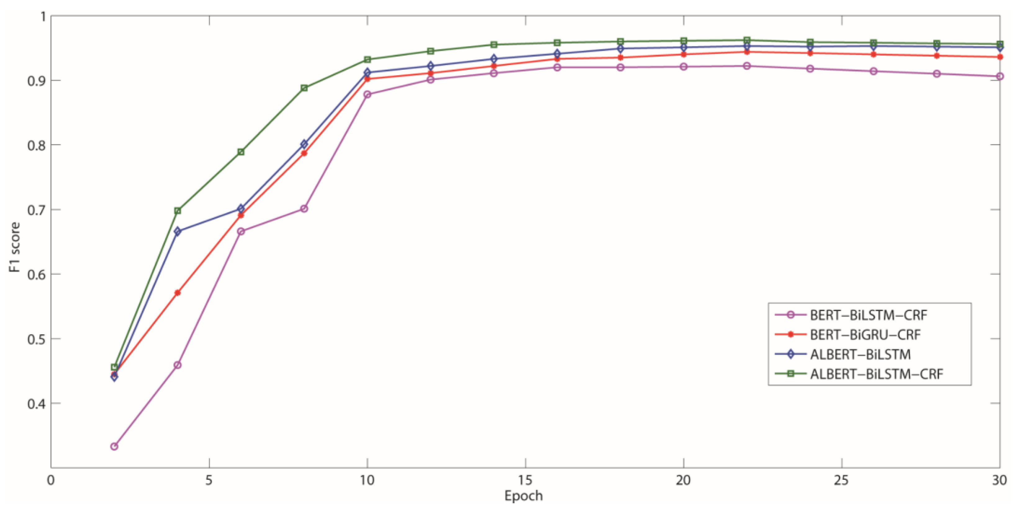
To better verify the performance of the TPCNER dataset and model, this paper also uses the BiLSTM–CRF, IDCNN–CRF, IDCNN–CRF2, BiLSTM–Attention–CRF, BERT–BiLSTM–CRF, BERT–BiGRU–CRF, ALBERT–BiLSTM, and ALBERT–BiLSTM–CRF models to test on the Boson dataset, MSRA dataset, and RenMinRiBao dataset and uses precision, recall, and F1-scores to evaluate the named entity recognition performance. The experimental results are shown in

Table 11. Results of models on the Boson, MSRA, and RenMinRiBao datasets.

Models	Boson			MSRA			RenMinRiBao
	Precision	Recall	F1-Score	Precision	Recall	F1-Score	Precision	Recall	F1-Score
BiLSTM–CRF	0.887	0.791	0.836	0.901	0.859	0.876	0.922	0.915	0.918
IDCNN–CRF	0.891	0.809	0.848	0.979	0.777	0.866	0.931	0.933	0.932
IDCNN–CRF2	0.912	0.909	0.910	0.980	0.771	0.863	0.934	0.941	0.937
BiLSTM–Attention–CRF	0.922	0.917	0.919	0.973	0.765	0.841	0.953	0.960	0.956
BERT–BiLSTM–CRF	0.932	0.933	0.932	0.974	0.813	0.886	0.961	0.965	0.963
BERT–BiGRU–CRF	0.941	0.945	0.943	0.979	0.822	0.894	0.976	0.971	0.973
ALBERTour–BiLSTM	0.951	0.956	0.953	0.981	0.881	0.928	0.981	0.979	0.980
ALBERTour–BiLSTM–CRF	0.961	0.962	0.961	0.989	0.895	0.940	0.976	0.986	0.981

. The experimental results show that these eight models achieve good results on these three datasets. Compared with the other seven models, the ALBERT–BiLSTM–CRF model has the best performance. Its precision, recall, and F1-score of the three datasets are higher than those of the other models. Compared with the three public datasets, the named entity recognition effect of the TPCNER dataset is basically the same, reaching more than 95%. In addition, this paper also counts and visualizes the F1-score of the BERT–BiLSTM–CRF, BERT–BiGRU–CRF, ALBERT–BiLSTM, and ALBERT–BiLSTM–CRF models after hyperparameter tuning, as shown in Figure 6. It can be clearly seen from the figure that the F1-score of the ALBERT–BiLSTM–CRF model is significantly higher than that of the other four models.

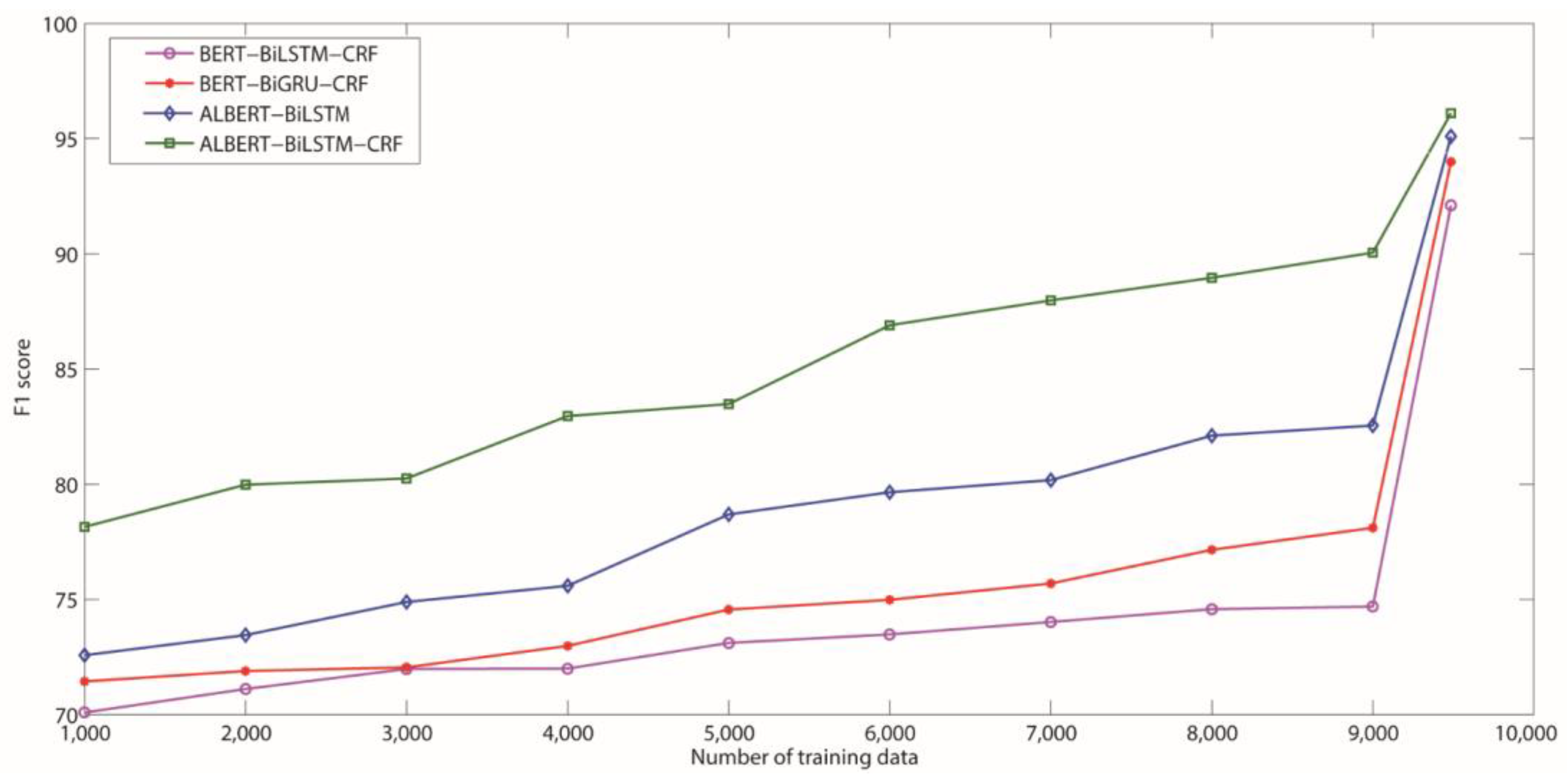
A total of 36 controlled experiments were performed to determine the best number of labeled phrases from the created dataset and to analyze the size of the labeled dataset. The first trial used 1000 sentences, whereas the remaining tests used a range of 2000 to 9000 sentences (with a step size of 1000). Figure 7 depicts the experimental outcomes in terms of average accuracy and recall.

As seen in Figure 7, when 9000 sentences were used, the proposed algorithm achieved an average F1-score of 96.2%. The BERT–BiLSTM–CRF, BERT–BiGRU–CRF, and ALBERT–BiLSTM (the baseline) only achieved F1-scores of 92.1%, 94.4%, and 95.3%, respectively. This shows that the proposed NER algorithm outperforms the baseline.

5.5. Ablation Analysis

To verify the effectiveness of pretraining on our approach, we design the following variant models and conduct experiments on the constructed dataset (see

Table 12. Experimental performance of variant models on the TPCNER dataset.

Model	Precision	Recall	F1-Score
BiLSTM–CRF	0.979	0.766	0.860
+BERT	0.928	0.915	0.921
+ALBERTold	0.925	0.844	0.883
+ALBERTour	0.961	0.962	0.961

).

Table 9 show the experimental results of BiLSTM–CRF as a baseline method. In Table 9, the performance of BiLSTM–CRF in all evaluation metrics is poor, compared with other models. Moreover, from the overall model F1-score in Table 9, we found that the use of the BERT layer or the use of ALBERT layer is higher than the baseline method. This phenomenon shows the effectiveness of the combination of pretraining model.

Compared with BiLSTM–CRF, the F1 value of the model can be improved by using pretraining model (BERT) in Table 9. The reason may be that pretraining enables better characterization of text sequence features. This phenomenon shows the effectiveness of using pretraining model.

Compared with Bi-LSTM–CRF, the model using spatial attention has improved in regard to the P, R, and F1-score in Table 9. The reason may be that domain pretrained models can better characterize geographic text features and then improves the extraction ability of BiLSTM encoding features. This phenomenon shows the effectiveness of using geographic pretraining model.

5.6. Discussion

5.6.1. Ablation Study

We focused on analyzing the constructed dataset (TPCNER). We examined an example from the TPCNER corpus to see if the provided model could better detect items in the geographic domain. In this example, the entity “Gulou Hospital of Harbin Engineering University” appeared just twice in the training set. The entity “Gulou Hospital of Harbin Engineering University” is recognized by the BERT–BiLSTM–CRF model as two entities, “Harbin Engineering University” and “Gulou Hospital”, as shown in

Table 13. Results of an instance being predicted by different models. B represents begin, I represents inside, E represents end, and O represents other.

Original sentence	黑龙江中部出现强降雨，其中哈尔滨工程大学古楼医院周边伴有冰雹。
Sentence translation	Heavy rainfall in central Heilongjiang, including hail in Harbin Yilan County.
Sentence pinyin (Chinese romanization)	Hei Long Jiang Zhong Bu Chu Xian Qiang Jiang Yu, Qi Zhong Ha Er Bin Gong Cheng Da Xue Gu Lou Yi Yuan Zhou Bian Ban You Bing Bao.
Correct Label	Hei/B–L long/I–L jiang/E–L zhong/O bu/O di/O qu/O chu/O xian/O qiang/O jiang/O yu/O, /O qi/O zhong/ha/B–L er/I–L bin/I–L gong/I–L cheng/I–L da/I–L xue/I–L gu/I–L lou/I–L yi/I–L yuan/E–L zhou/O bian/O ban/O you/O bing/O bao/O. /O
b	Hei/B–L long/I–L jiang/E–L zhong/O bu/O di/O qu/O chu/O xian/O qiang/O jiang/O yu/O, /O qi/O zhong/ha/B–L er/I–L bin/I–L gong/I–L cheng/I–L da/I–L xue/E–L gu/B–L lou/I–L yi/I–L yuan/E–L zhou/O bian/O ban/O you/O bing/O bao/O. /O
BERT–BiGRU–CRF predict	Hei/B–L long/I–L jiang/E–L zhong/O bu/O di/O qu/O chu/O xian/O qiang/O jiang/O yu/O, /O qi/O zhong/ha/B–L er/I–L bin/I–L gong/I–L cheng/I–L da/I–L xue/E–L gu/B–L lou/I–L yi/I–L yuan/E–L zhou/O bian/O ban/O you/O bing/O bao/O. /O
ALBERTours–BiLSTM predict	Hei/B–L long/I–L jiang/E–L zhong/O bu/O di/O qu/O chu/O xian/O qiang/O jiang/O yu/O, /O qi/O zhong/ha/B–L er/I–L bin/I–L gong/I–L cheng/I–L da/I–L xue/E–L gu/B–L lou/I–L yi/I–L yuan/E–L zhou/O bian/O ban/O you/O bing/O bao/O. /O
ALBERTours–BiLSTM–CRF predict	Hei/B–L long/I–L jiang/E–L zhong/O bu/O di/O qu/O chu/O xian/O qiang/O jiang/O yu/O, /O qi/O zhong/ha/B–L er/I–L bin/I–L gong/I–L cheng/I–L da/I–L xue/I–L gu/I–L lou/I–L yi/I–L yuan/E–L zhou/O bian/O ban/O you/O bing/O bao/O. /O

. Because these two items are more abundant in the training set, recognition without augmentation information will be deceptive. Because of inaccurate boundary information, the BERT–BiLSTM–CRF model wrongly classifies “Gulou Hospital of Harbin Engineering University” as an entity. Because more extensive augmentation information is incorporated into our suggested model, it provides accurate predictions. Furthermore, the terms “Harbin Engineering University” and “Gulou Hospital” in the sample are similar, implying a tighter relationship between the entity’s characteristics.

5.6.2. Error Analysis

We chose many sentences from the testing set and assessed their sample mistakes to evaluate the real output of different models. Figure 8 shows the recognition results of the BERT–BiLSTM–CRF, BERT–BiGRU–CRF, ALBERT–BiLSTM, and ALBERT–BiLSTM–CRF models in sample texts, where the red characters denote errors.

As demonstrated in Figure 8, our model outperformed the others in terms of recognition, whereas the BERT–BiLSTM–CRF model failed to distinguish nested entities. For instance, the ALBERT–BiLSTM–CRF recognized “Yang Xinhe” as an entity in Case 1, but other models cannot recognize this entity because it is a place name consisting of a person’s name, and many algorithms will recognize the person’s name. In Case 2, the BERT–BiLSTM–CRF identifies “Horqin” as an entity, but the related characters “Right Wing Front Banner Debs Town” placed at a long distance in the context were missed. The ALBERT–BiLSTM–CRF model successfully identified the fine-grained nested entities “Deebs Township, Horqin Right Wing Front Banner” in Case 2.

By analyzing the recognition results, we found that (1) the reason for affecting the accuracy of the model is that some of the names in the data contain toponymic words, resulting in incorrect recall, e.g., “Yang Xinhe” and “Li Qingxian”; (2) the reason for the low recall is that some of the complex names are not correctly recognized, e.g., “Deebs Town of Horqin Right-wing Front Banner” is not correctly recognized. For example, in “wind and hail disaster caused crop collapse in Debs town of horqin right-wing front banner”, “Debs town of horqin right-wing front banner” was not correctly identified; in the face of rain and flood, Qiongzhong Li and Miao autonomous county urgently relocated. The name “Qiongzhong Li and Miao Autonomous County” was not correctly identified in “35 people”. The reason is that the place name is long, the frequency of occurrence in the corpus is low, and the model does not learn enough, so it is not correctly recalled.

5.6.3. Annotated Quality Analysis

BiLSTM–CRF and IDCNN are considered the most basic models and were used to assess the quality of the annotated corpus, using hierarchical 10-fold cross-validation [36,37]. At the macro level, the detailed experimental results presented in Table 6 show that BiLSTM–CRF and IDCNN achieve F1-scores of 86% and 87%, respectively. At the micro level, BiLSTM–CRF and IDCNN show excellent performance for traffic, water systems, and organization, thus indicating the ease of identification of these categories. In particular, for organizational agencies, the F1-score of both models is 92.16% and 93.79%, respectively. Due to discrepancies created by the absence of boundary characteristics and the mixed usage of characters, digits, and letters, some things, such as extremely specified place names, mixed place names, and merged place names, are difficult to recognize. Figure 2 demonstrated how the lack of data for some categories has an impact on performance. In addition, as indicated in Figure 5, we mentioned several forecast mistakes. Overall, the assessment findings show that the corpus annotated in this study is reliable and may be utilized to recognize geographic domain entities.

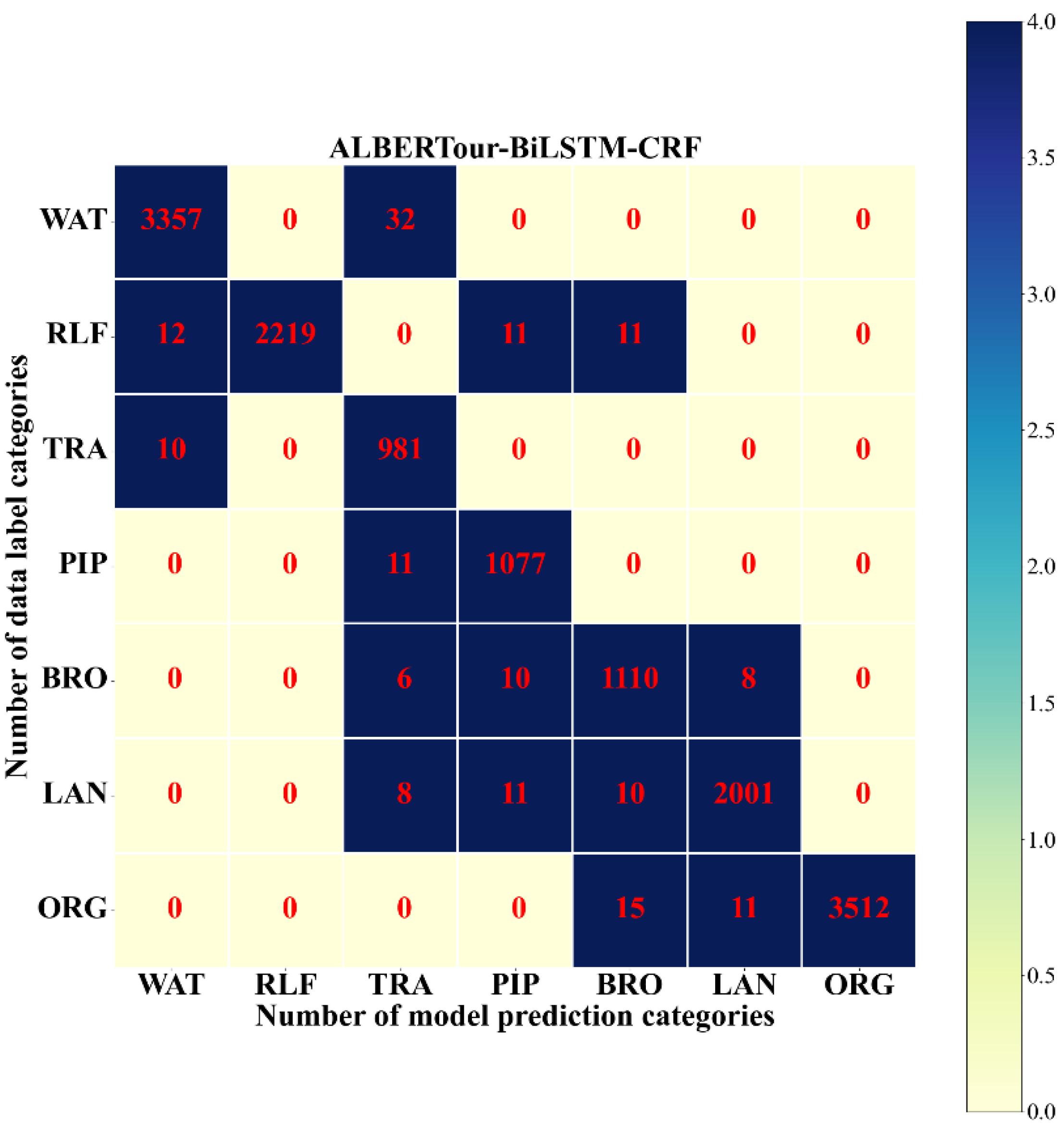
The confusion matrix in Figure 9 and Figure 10 shows the number of toponyms that were extracted from the dataset by using the proposed algorithm, as well as the number of gold-standard annotations, for each toponym class. Figure 10 shows that the proposed algorithm has a relatively lower precision for the TRA toponym classes. This could be attributed to data imbalance. The imbalance in entity number causes the algorithm to focus on minimizing classification errors for the entities with a larger number, while insufficiently considering the errors for the entities with a smaller number.

6. Conclusions and Future Work

In this paper, we propose a hybrid neural network method for Chinese place-name recognition that solves the above problems by learning word-level feature representations in the ALBERT layer, extracting contextual semantic features in the BiLSTM layer, and generating optimal label sequences in the CRF layer. The experimental results show that the proposed toponym recognition method has good performance in all evaluation indices. We train ALBERT–BiLSTM–CRF by using a constructed human-annotated dataset and three public datasets. We experimented with several training procedures and discovered that a mix of human-annotated data produces the greatest results. Evaluation experiments based on three test datasets, namely Boson, MSRA, and RenMinRiBao, demonstrate the improved performance of ALBERT–BiLSTM–CRF in comparison with a set of deep learning models. This work attempted to serve as a resource for named-entity-recognition studies in various geographic areas. We will work on including more features and making more sensible modifications to the weights of these features in the future.

References

1. Imran, M.; Castillo, C.; Diaz, F.; Vieweg, S. Processing social media messages in mass emergency: A survey. ACM Comput. Surv. 2015, 47, 67. [Google Scholar] [CrossRef]
2. Silverman, L. Facebook, Twitter Replace 911 Calls for Stranded in Houston. 2017. Available online: https://www.npr.org/sections/alltechconsidered/2017/08/28/546831780/texas-police-and-residents-turn-to-social-media-to-communicateamid-harvey (accessed on 12 September 2017).
3. Yu, M.; Huang, Q.; Qin, H.; Scheele, C.; Yang, C. Deep learning for real-time social media text classification for situation awareness—Using hurricanes Sandy, Harvey, and Irma as case studies. Int. J. Digit. Earth 2019, 12, 1230–1247. [Google Scholar] [CrossRef]
4. Hu, Y.; Mao, H.; McKenzie, G. A natural language processing and geospatial clustering framework for harvesting local place names from geotagged housing advertisements. Int. J. Geogr. Inf. Sci. 2018, 33, 714–738. [Google Scholar] [CrossRef] [Green Version]
5. Freire, N.; Borbinha, J.; Calado, P.; Martins, B. A metadata geoparsing system for place name recognition and resolution in metadata records. In Proceedings of the 11th International ACM/IEEE Joint Conference on Digital Libraries, Ottawa, ON, Canada, 13–17 June 2011; pp. 339–348. [Google Scholar]
6. Gelernter, J.; Balaji, S. An algorithm for local geoparsing of microtext. Geoinformatica 2013, 17, 635–667. [Google Scholar] [CrossRef]
7. Gritta, M.; Pilehvar, M.T.; Limsopatham, N.; Collier, N. What’s missing in geographical parsing? Lang. Resour. Eval. 2018, 52, 603–623. [Google Scholar] [CrossRef] [Green Version]
8. Jones, C.B.; Purves, R.S. Geographical information retrieval. Int. J. Geogr. Inf. Sci. 2008, 22, 219–228. [Google Scholar] [CrossRef]
9. Purves, R.S.; Clough, P.; Jones, C.B.; Hall, M.H.; Murdock, V. Geographic Information Retrieval: Progress and Challenges in Spatial Search of Text. Found. Trends® Inf. Retr. 2018, 12, 164–318. [Google Scholar] [CrossRef]
10. Derczynski, L.; Nichols, E.; Van Erp, M.; Limsopatham, N. Results of the WNUT2017 shared task on novel and emerging entity recognition. In Proceedings of the Third Workshop on Noisy User-Generated Text, Copenhagen, Denmark, 7 September 2017; pp. 140–147. [Google Scholar]
11. Li, H.; Wang, M.; Baldwin, T.; Tomko, M.; Vasardani, M. UniMelb at SemEval-2019 Task 12: Multi-model combination for toponym resolution. In Proceedings of the 13th International Workshop on Semantic Evaluation, Minneapolis, MN, USA, 6–7 June 2019; ACL: Stroudsburg, PA, USA; pp. 1313–1318. [Google Scholar]
12. Qiu, Q.; Xie, Z.; Wu, L.; Tao, L.; Li, W. BiLSTM-CRF for geological named entity recognition from the geoscience literature. Earth Sci. Inform. 2019, 12, 565–579. [Google Scholar] [CrossRef]
13. Qiu, Q.; Xie, Z.; Wu, L.; Tao, L. GNER: A generative model for geological named entity recognition without labeled data using deep learning. Earth Space Sci. 2019, 6, 931–946. [Google Scholar] [CrossRef] [Green Version]
14. Santos, R.; Murrieta-Flores, P.; Calado, P.; Martins, B. Toponym matching through deep neural networks. Int. J. Geogr. Inf. Sci. 2018, 32, 324–348. [Google Scholar] [CrossRef]
15. Wang, J.; Hu, Y. Enhancing spatial and textual analysis with EUPEG: An extensible and unified platform for evaluating geoparsers. Trans. GIS 2019, 23, 1393–1419. [Google Scholar] [CrossRef]
16. Herskovits, A. Language and Spatial Cognition: An interdisciplinary Study of Prepositions in English; Cambridge University Press: Cambridge, UK, 1986. [Google Scholar]
17. Talmy, L. Toward a Cognitive Semantics: Concept Structuring Systems; The MIT Press: Cambridge, MA, USA, 2000. [Google Scholar]
18. Stock, K.; Yousaf, J. Context-aware automated interpretation of elaborate natural language descriptions of location through learning from empirical data. Int. J. Geogr. Inf. Sci. 2018, 32, 1087–1116. [Google Scholar] [CrossRef]
19. Cohen, W.; Ravikumar, P.; Fienberg, S. A comparison of string distance metrics for namematching tasks. In Proceedings of KDD Workshop on Data Cleaning and Object Consolidation, Washington, DC, USA, 24–27 August 2003. [Google Scholar]
20. Moreau, E.; Yvon, F.; Capp, E.O. Robust similarity measures for named entities matching. In Proceedings of the International Conference on Computational Linguistics, Manchester, UK, 18–22 August 2008. [Google Scholar]
21. Santos, R.; Murrieta-Flores, P.; Martins, B. Learning to combine multiple string similarity metrics for effective toponym matching. Int. J. Digit. Earth 2018, 11, 913–938. [Google Scholar] [CrossRef]
22. Ma, K.; Tan, Y.; Tian, M.; Xie, X.; Qiu, Q.; Li, S.; Wang, X. Extraction of temporal information from social media messages using the BERT model. Earth Sci. Inform. 2022, 15, 573–584. [Google Scholar] [CrossRef]
23. Qiu, Q.; Xie, Z.; Ma, K.; Chen, Z.; Tao, L. Spatially oriented convolutional neural network for spatial relation extraction from natural language texts. Trans. GIS 2021, 26, 839–866. [Google Scholar] [CrossRef]
24. Qiu, Q.; Xie, Z.; Ma, K.; Chen, Z.; Tao, L. Spatially oriented convolutional neural network for spatial relation extraction from natural language texts. Trans. GIS 2022, 26, 839–866. [Google Scholar] [CrossRef]
25. Devlin, J.; Chang, M.W.; Lee, K.; Toutanova, K. Bert: Pre-training of deep bidirectional transformers for language understanding. arXiv 2018, arXiv:1810.04805. [Google Scholar]
26. Radford, A.; Wu, J.; Child, R.; Luan, D.; Amodei, D.; Sutskever, I. Language models are unsupervised multitask learners. OpenAI blog 2019, 1, 9. [Google Scholar]
27. Ling, W.; Dyer, C.; Black, A.W.; Trancoso, I. Two/too simple adaptations of word2vec for syntax problems. In Proceedings of the 2015 Conference of the North American Chapter of the Association for Computational Linguistics: Human Language Technologies, Denver, CO, USA, May–June 2015; pp. 1299–1304. [Google Scholar]
28. Lv, X.; Xie, Z.; Xu, D.; Jin, X.; Ma, K.; Tao, L.; Qiu, Q.; Pan, Y. Chinese Named Entity Recognition in the Geoscience Domain Based on BERT. Earth Space Sci. 2022, 9, e2021EA002166. [Google Scholar] [CrossRef]
29. Ma, K.; Tian, M.; Tan, Y.; Xie, X.; Qiu, Q. What is this article about? Generative summarization with the BERT model in the geosciences domain. Earth Sci. Inform. 2021, 15, 21–36. [Google Scholar] [CrossRef]
30. Lan, Z.; Chen, M.; Goodman, S.; Gimpel, K.; Sharma, P.; Soricut, R. Albert: A lite bert for self-supervised learning of language representations. arXiv 2019, arXiv:1909.11942. [Google Scholar]
31. Hochreiter, S.; Schmidhuber, J. Long short-term memory. Neural Comput. 1997, 9, 1735–1780. [Google Scholar] [CrossRef]
32. Graves, A. Long short-term memory. In Supervised Sequence Labelling with Recurrent Neural Networks; Springer: Berlin/Heidelberg, Germany, 2012; pp. 37–45. [Google Scholar]
33. Qiu, Q.; Xie, Z.; Wu, L.; Li, W. DGeoSegmenter: A dictionary-based Chinese word segmenter for the geoscience domain. Comput. Geosci. 2018, 121, 1–11. [Google Scholar] [CrossRef]
34. Song, S.; Zhang, N.; Huang, H. Named entity recognition based on conditional random fields. Clust. Comput. 2017, 22, 5195–5206. [Google Scholar] [CrossRef]
35. Guo, X.; Zhou, H.; Su, J.; Hao, X.; Tang, Z.; Diao, L.; Li, L. Chinese agricultural diseases and pests named entity recognition with multi-scale local context features and self-attention mechanism. Comput. Electron. Agric. 2020, 179, 105830. [Google Scholar] [CrossRef]
36. Leitner, E.; Rehm, G.; Moreno-Schneider, J. A dataset of german legal documents for named entity recognition. arXiv 2020, arXiv:2003.13016. [Google Scholar]
37. Wang, S.; Zhang, X.; Ye, P.; Du, M. Deep Belief Networks Based Toponym Recognition for Chinese Text. ISPRS Int. J. Geo-Inf. 2018, 7, 217. [Google Scholar] [CrossRef] [Green Version]
38. Wang, X.; Ma, C.; Zheng, H.; Liu, C.; Xie, P.; Li, L.; Si, L. DM NLP at SemEval 2018 Task 12: A pipeline system for toponym resolution. In Proceedings of the 13th International Workshop on Semantic Evaluation, Minneapolis, MN, USA, 6–7 June 2019; pp. 917–923. [Google Scholar]
39. Wang, J.; Hu, Y.; Joseph, K. NeuroTPR: A neuro-net toponym recognition model for extracting locations from social media messages. Trans. GIS 2020, 24, 719–735. [Google Scholar] [CrossRef]
40. Ma, K.; Tan, Y.; Xie, Z.; Qiu, Q.; Chen, S. Chinese toponym recognition with variant neural structures from social media messages based on BERT methods. J. Geogr. Syst. 2022, 24, 143–169. [Google Scholar] [CrossRef]
41. Qiu, Q.; Xie, Z.; Wang, S.; Zhu, Y.; Lv, H.; Sun, K. ChineseTR: A weakly supervised toponym recognition architecture based on automatic training data generator and deep neural network. Trans. GIS 2022, 26, 1256–1279. [Google Scholar] [CrossRef]
42. Hu, X.; Zhou, Z.; Sun, Y.; Kersten, J.; Klan, F.; Fan, H.; Wiegmann, M. GazPNE2: A General Place Name Extractor for Microblogs Fusing Gazetteers and Pretrained Transformer Models. IEEE Internet Things J. 2022, 9, 16259–16271. [Google Scholar] [CrossRef]
Figure 1. Overall workflow of ChineseNERAnno.
Ijgi 11 00598 g001
Figure 2. Distribution for each category in TPCNER.
Ijgi 11 00598 g002
Figure 3. The overall architecture of the proposed model.
Ijgi 11 00598 g003
Figure 4. Basic structure of the ALBERT model.
Ijgi 11 00598 g004
Figure 5. Neuron structure of LSTM.
Ijgi 11 00598 g005
Figure 6. The F1-scores of each model after hyperparameter tuning.
Ijgi 11 00598 g006
Figure 7. Average F1-score of the presented and baseline NER algorithms with different sizes of labeled data.
Ijgi 11 00598 g007
Figure 8. Error analysis of some typical cases. Blue represents standard place-name labeling, and red represents model identification place names. The translation of the sentence “杨信河以北的李庆县发生了特大暴雨” is “Very heavy rainfall occurred in Liqing County north of Yang Xin River”; the translation of the sentence “风雹灾害致科尔沁右翼前旗德伯斯镇作物倒伏” is “Wind and hail disaster caused the Khorqin Right Wing Front Banner Debs town crop collapse”.
Ijgi 11 00598 g008
Figure 9. Confusion matrix for all extracted and gold-standard toponym from the constructed dataset based on ALBERT–BiLSTM–CRF. WAT = water system; RLF = residential land and facilities; TRA = transportation; PIP = pipelines; BRO = boundaries, regions, and other areas; LAN = landforms; ORG = organization.
Ijgi 11 00598 g009
Figure 10. Confusion matrix for all extracted and gold-standard toponym from the constructed dataset based on ALBERT–BiLSTM–CRF. WAT = water system; RLF = residential land and facilities; TRA = transportation; PIP = pipelines; BRO = boundaries, regions, and other areas; LAN = landforms; ORG = organization.
Ijgi 11 00598 g010