Abstract
In recent years, deep learning has become the mainstream development direction in the change-detection field, and its accuracy and speed have also reached a high level. However, the change-detection method based on deep learning cannot predict all the change areas accurately, and its application is limited due to local prediction defects. For this reason, we propose an interactive change-detection network (ICD) for very high resolution (VHR) based on a deep convolution neural network. The network integrates positive- and negative-click information in the distance layer of the change-detection network, and users can correct the prediction defects by adding clicks. We carried out experiments on the open source dataset WHU and LEVIR-CD. By adding clicks, their F1-scores can reach 0.920 and 0.912, respectively, which are 4.3% and 4.2% higher than the original network. To better evaluate the correction ability of clicks, we propose a set of evaluation indices—click-correction ranges, which is suitable for evaluating clicks, and we carry out experiments on the above models. The results show that the method of adding clicks can effectively correct the prediction defects and improve the result accuracy.
1. Introduction
Change detection is the process to identify the changes in objects in the same area at two different times [1]. At present, it is widely used in natural-disaster damage assessment, land-use monitoring, medical diagnosis and treatment, underwater measurement and other fields. Traditional change detection is mainly used for very high-resolution (VHR) remote-sensing images. Most of the early change-detection methods are direct pixel-comparison methods, such as the direct comparison method, image transformation method, and post-classification comparison method [2,3,4,5]. The essence of these methods is to extract change information through pixel-by-pixel comparison, which has good applicability in early low-resolution image change detection. However, this method is sensitive to noise, error and other factors, with poor robustness and a high false detection rate.
To better extract all kinds of ground features in images, many scholars use machine-learning technology to achieve higher change detection accuracy with more rigorous mathematical calculations, such as support-vector machines [6,7], decision-tree methods [8,9], and random forest methods [10,11]. To adapt to the development of high spatial-resolution, remote-sensing image change detection, based on the object-oriented image analysis strategy, with the help of level sets [12], Markov random fields [13], conditional random fields [14] and other methods, many scholars classify the images of different phases and then compare and analyze the various object information to obtain the change results of the two image phases. Although this kind of method can extract the complete change information, it requires high image resolution and has low generalization ability. In recent years, with the rapid development of deep learning and big data technology, remote-sensing image change detection methods based on deep convolutional neural networks [15], such as STANet [16], DASNet [17], SSCDNet [18], and SRCDNet [19], have gradually become mainstream. Due to the complex structure and large number of computations in deep-learning networks, the network can automatically detect changes in objects and compared with other detection strategies, its accuracy and scalability significantly improve. To a certain extent, it also avoids the problems of traditional remote-sensing interpretation, such as partial homologous and heterospectral foreign matter. Although accuracy and generalization have improved, the change-detection method based on deep learning is more sensitive to factors such as sample size, sample fineness and image resolution. The model performance is different on different images, and the detection effect often lags behind the ideal effect. To improve the detection accuracy of the change-detection network on different images, one of the simplest and most direct methods is to modify the detection results interactively. In the past, correcting predicted results often relied on manual intervention, and the correction process was complicated and lengthy. Additionally, the time and labor costs of interaction were also relatively high. Therefore, we intend to explore a new interactive mechanism to simplify the correction process of change detection results and refine the change detection results to improve efficiency.
Interactive segmentation is a method for modifying the detection results by inputting external interaction information. In the past, this method was usually used for training semisupervised image-segmentation models [20,21]. During model training, the user drew marks on the samples to guide the training direction of the model. This method can reduce the labeling of original samples and improve the training accuracy of unsupervised or semisupervised image-segmentation models. In recent years, with the rise of deep-learning methods, many scholars have studied interactive segmentation methods based on deep learning. Sofiiuk [22] integrated click information into an image segmentation network, used deep learning to extract the features of user interactive clicks and image objects, and refined the segmentation range. Zhang [23] proposed an interactive target-segmentation algorithm based on a two-stage network, which generates interactive information by flexible painting interaction, making the results more complete, and refined. Castrejon [24] proposed a semi-automatic target instance annotation algorithm. According to the target frame provided by the user, the circular neural network is used to iterate the polygon vertices of the target object in the frame to obtain more accurate segmentation results. These interactive segmentation methods based on deep learning can not only be applied to training semisupervised image segmentation models, but can also modify the existing detection results. Therefore, this interactive segmentation method using deep learning can solve the problem of cumbersome detection result correction.
However, research on interactive change detection is still in its infancy. Most of the existing studies on interactive change detection focus on training semisupervised classification models to reduce the labeling of original samples [25,26,27,28]. This kind of interaction strategy can only improve the model accuracy or reduce the number of manually labeled samples, but it cannot modify the change detection results twice. The interaction degree is limited, and it is difficult to modify the existing detection results. At present, there are few interactive change-detection studies based on deep learning, so research on this aspect is worth exploring. In the image-segmentation field, the essence of the interactive segmentation method based on deep learning is to transfer the interaction information provided by the user into the neural network. For example, some scholars take the Euclidean distance from all pixel points to the interaction points as the interaction map and take it and the original image as the initial input of the network [29,30]. This method not only simplifies the interaction, but also ensures high segmentation accuracy. To further simplify the interaction process, some scholars convolve the interaction layer separately [31] and add the weight of the interaction layer and the image-feature map as the subsequent input. Compared with the former, this method increases the impact of user interaction. The above method of modifying the prediction result by introducing the click weight provides an interactive idea for our change detection method based on deep learning.
Therefore, to further deepen the degree of human-computer interaction in a change-detection network based on deep learning, we incorporate clicks into the change-detection network, add the weights of positive and negative clicks to the distance layer of the network, and extract the features again to achieve the effect of using clicks to modify the prediction results. Thus, an interactive change-detection (ICD) network for VHR remote-sensing images based on a deep convolutional neural network is realized. Figure 1 shows the result correction process based on the ICD network. The purple patch on the left is the patch to be corrected before prediction, and the green patch on the right is the corrected patch. Among them, the buildings on the left of the first row are not fully predicted. After adding positive clicks (the yellow dot in Figure 1), which can make up for patches that are not fully predicted, the complete building is predicted. At the same time, the image on the left side of the second row has a false detection, and the nonbuilding patch is predicted. After adding negative clicks (the blue dot in Figure 1), which can delete patches of prediction error, the redundant prediction part is deleted.
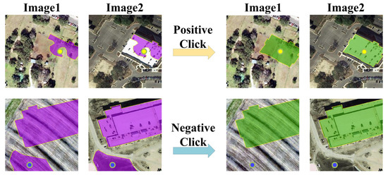
Figure 1.
Schematic diagram of interactive change detection and correction.
2. Materials and Methods
To realize interactive change detection based on deep learning, we make two improvements to the original change detection network. (1) We modify the training process. In the training process, the generation process of positive and negative clicks is introduced so that each generation of the model has the click matching the prediction results of the previous generation model. (2) We modify the network structure. The weights of positive and negative clicks are added to the distance layer of the network; secondary feature extraction is carried out, and the modified prediction results are obtained.
2.1. Structure of the Interactive Change Detection Network
We propose an interactive change-detection network and introduce positive and negative clicks so that the network can modify the original prediction results according to these clicks, thereby achieving the interactive segmentation effect. Figure 2 shows the network structure of the ICD approach.
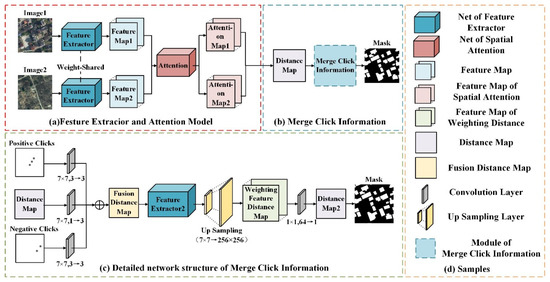
Figure 2.
ICD network structure.
Figure 2a shows the module of the feature extraction and attention mechanism. The feature-extraction module is ResNet18, which does not include the global pooling layer and the fully connected layer. The dual temporal images share the same weight in feature extraction, and the PAM [16] module is used in the attention mechanism module, which can extract more detailed, global, spatiotemporal relationships. After extracting the feature information of the two images, we make a difference between the two and obtain a preliminary feature distance map. In the common change-detection network, the final prediction result can be obtained by filtering the threshold of the feature distance graph in the above results. However, in the interactive change detection ICD, we will also fuse the click information of the feature distance graph. Figure 2b shows the fusion position of clicks. The generation and fusion of clicks are described in Section 2.2.
Figure 2c shows a detailed network structure integrating click information. In terms of the fusion mode, we refer to Conv1s Figure 3a in paper [22], which performs convolution operations on clicks and pictures to turn them into the same channel, fuses them, and finally performs feature extraction in a unified manner. In ICD, since the network is a dual stream structure, if clicks and pictures are merged at the beginning (Figure 3b), the impact of clicks will offset each other when calculating the difference between two pictures. Therefore, clicks cannot enter the network together with the pictures at the beginning. Since the point to be corrected by the clicks is the change area between the two pictures, we will start with the distance map (purple module in Figure 3c) indicating the change and integrate the clicks with this part. First, a 7 × 7 convolution operation is performed on the characteristic distance map and 1 channel is converted to 3 channels to fit the channel number of clicks. Next, a 7 × 7 convolution operation is performed on the positive and negative click maps to unify the two dimensions with the feature distance map. Then, by adding the weights of the feature distance map and the positive and negative clicks, a fusion distance map X is obtained, which integrates the click information. Then, X is sent into a new feature extraction network for a new round of feature extraction, and the result of feature extraction is sampled up to make it from 7 × 7 to 256 × 256 and the new feature distance map X’ is obtained. Finally, a 1 × 1 convolution operation on X’ is performed to convert 64 channels to 1 channel and perform a threshold filter, and then the final mask result can be obtained.
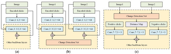
Figure 3.
Methods of fusing clicks. (a) Conv1S; (b) merge at the beginning; (c) merge at the distance map.
In the above process, we connected ResNet after the click integration to better extract the correction information brought by clicks. However, unlike the interactive segmentation method of the single stream network, in the dual-stream network such as ICD, the change information of the two pictures is extracted and processed many times before the click fusion. If the feature extraction is performed again at this time, the effect may not be better than that of only convolution feature fusion. Therefore, to verify the effectiveness of secondary feature extraction, we carried out corresponding experiments in Section 3.2.
2.2. Automatic Generation of Clicks
In the training process, starting from the second generation model, we need to automatically select the clicks according to the prediction results of the last model to provide a real-time reference for the training of this round of click correction ability. Algorithm 1 shows the automatic generation steps of clicks.
| Algorithm 1 Automatic generation algorithm of clicks. |
| Input: The latest generation model, two-phase training samples A, B and the corresponding label; Output: Positive Clicks and Negative Clicks for current model training results. |
| 1: Use the model to predict the training samples, and obtain the prediction results; 2: Compare the prediction results with the labels to determine the areas that need to be modified by positive and negative clicks. These areas are defined as follows:
4: Use connected components to divide the pixels of False Negative and False Positive into different clusters, and obtain the cluster sets F.N.Set and F.P.Set, respectively; 5: Determine the first N large areas maxN(F.N.Set) and maxN(F.P.Set) of F.N.Set and F.P.Set according to the number of pixels; 6: Take the centroid in maxN(F.N.Set) and maxN(F.P.Set) as Positive Clicks and Negative Clicks, respectively; |
| 7: Update the Positive Clicks and Negative Clicks of the training samples; 8: Return Positive Clicks and Negative Clicks. |
In the initial training process, because there is no reference image to be corrected, we set the positive and negative clicks to be empty. After the first-generation model training is completed, all training samples are predicted based on this, and the prediction results (Figure 4a1) are compared with the original label (Figure 4a2) to determine the part that is actually changed, but not predicted (Figure 4a3), and the part that is actually unchanged, but predicted (Figure 4a4). The two parts correspond to the areas that need to be corrected for the positive and negative clicks.
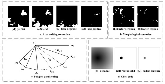
Figure 4.
Schematic diagram of the click generation algorithm.
Then, to correct the whole population of points in the area to be corrected and avoid the situation in which the selected points are located in the boundary, we need to carry out morphological corrosion on the extracted area to be corrected and refine and narrow the click-extraction range. Morphological etching refers to convolving the original image and taking the local minimum value. It can reduce the patch area from the boundary and eliminate the small clastic spots. The convolution kernel size used in our etching operation is 3 × 3, the number of iterations is 3, and the corrosion effect is shown in Figure 4b. Figure 4b1 shows the spots before corrosion, and the results after the corrosion operation are shown in Figure 4b2.
Next, according to the connected components, the pixels in the two are divided into different clusters, and the top N clusters are determined according to the number of pixels. To avoid the situation in which the cluster is too large due to the connection of different areas, we use the seed 4-connected algorithm when taking the connected components. After that, to quickly select the centers of these areas, we use the centroid extraction algorithm, which can account for the calculation speed and position accuracy. First, we use the Canny [32] algorithm to extract the boundary of each cluster point. After the boundary is extracted, the boundary points need to be arranged clockwise. Choose the mean center point of boundary points as the fixed corner point and then take another point in the horizontal direction on the left of to generate the horizontal vector . Then, traverse all boundary points , and calculate all angles between and (Equations (1)–(3)). Finally, after sorting the angle from small to large, the boundary points arranged clockwise can be obtained.
After sorting the boundary points clockwise, the centroid of the N areas to be corrected can be selected. Let an area to be corrected be any n-sided polygon with (, ) (i = 1,2…,n) as the vertex (Figure 4c). The area of each triangle is . The center of mass is (, ). The area of the polygon is S, and the centroid is G(x, y). The calculation formula is shown in Equations (4)–(9).
After selecting the clicks, the positive and negative clicks of each sample are generated according to a certain radius. Since the accuracy of the ordinary Euclidean distance graph (Figure 4d1) is not as accurate as the solid point with a certain radius (Figure 4d2) [22], we improved it (Equation (10)) so that the color of each click center is the deepest, decreases outward along the radius, and returns to the background color at the radius (Figure 4d3). This method can reduce the influence weight of the click edge and make the correction range more accurate. The experiment is described in Section 3.2.
2.3. The Evaluation Index
At present, the evaluation index of the existing change detection network, which evaluates the overall accuracy of the prediction results through multiangle calculation, is improved. Conventional change detection accuracy indicators include accuracy, precision, recall and F1-score. Accuracy is the ratio of the number of correctly divided samples to the number of all samples. The larger the accuracy value is, the more pixels are correctly detected. Precision is the ratio of the number of positive samples detected to the number of real positive samples. The higher the precision is, the more accurate the positive samples detected by the model. Recall is the ratio of the number of positive samples detected to the total number of positive samples. The higher the recall is, the more positive samples the model can find. The F1-score is the harmonic average of precision and recall, which is an important index to evaluate the performance of the model. The higher the F1-score is, the better the detection ability of the model as a whole. See Formulas (11)–(14) for the calculation of the above indexes:
where TP is the number of samples whose detection value is the same as the real value and whose detection value is positive, TN is the number of samples whose detection value is the same as the real value and whose detection value is negative, FP is the number of samples whose detection value is different from the real value and whose detection value is positive, and FN is the number of samples whose detection value is different from the real value and whose detection value is negative.
However, the prediction accuracy of the ICD network cannot be evaluated properly only by using the accuracy-evaluation index of the existing change-detection network. On the one hand, when evaluating the accuracy of the system, all the clicks are automatically simulated by the algorithm, and the correction position is not necessarily appropriate, so the correction effect is limited. On the other hand, the ICD network is different from the ordinary change-detection network. It not only needs to ensure the accuracy of the overall prediction results, but also the effectiveness of the click correction ability. However, the existing accuracy-evaluation system can only verify the accuracy of the former, and the latter cannot be evaluated effectively. To provide a more complete accuracy-evaluation system for the ICD network, we propose an index, the click correction range, which is suitable for evaluating the effect of click correction in the ICD network.
The click-correction range refers to the index used to evaluate the effect of click correction, which is divided into two types: positive click-correction range and negative click-correction range. They are used to evaluate the correction ability of positive and negative clicks.
- Correction range of positive clicks
The positive click is used to fill and correct the unpredicted change area, and its main correction position is in the actual change area. In this regard, we define the click-correction range as the ratio of the number of newly added changed pixels in the actual change area of the corrected click to the actual number of changed pixels to be corrected, as shown in Equation (15):
where is the correction range of positive clicks, N is the number of samples in all validation sets, is the number of changed pixels in the actual change area where the click is located (yellow area in Figure 5c), is the number of changed pixels in the actual change area where the click is located before correction (blue area in Figure 5b), and is the actual number of pixels in the area where the click is located (Figure 5a white area). The correction range of positive clicks reflects the correction ability of positive clicks, that is, the proportion of the area to be corrected after positive click correction.
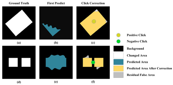
Figure 5.
Schematic diagram of click correction range parameters. (a,d) Ground Truth; (b,e) First Predict Result; (c,f) Click Correction Result.
- 2.
- Negative click-correction range
A negative click is used to eliminate and correct the error prediction area in the unchanged area, and the main correction position is in the actual unchanged area. In this regard, we define the click correction range of negative clicks as the ratio of the number of newly added unchanged pixels in the actual unchanged area where the correction click is located to the actual number of unchanged pixels to be corrected, as shown in Equation (16):
where is the negative click-correction range, N is the number of samples in all validation sets, is the number of unchanged pixels in the actual unchanged area where the correction click is located (black area in Figure 5), is the number of unchanged pixels in the actual unchanged area where the correction click is located before correction (black area in Figure 5e), and is the actual number of unchanged pixels where the correction click is located (black area in Figure 5d). A negative click-correction range reflects the correction ability of negative clicks, that is, the proportion of the area to be corrected after negative click correction.
2.4. Loss Function
In change detection, category imbalance is a common problem, because there is a large difference in the amount of information between unchanged information and changed information in these two images, and the changed information generally only accounts for a small part of all information. Such problems can be adjusted by setting the loss function to achieve the balance of changing information.
Batch-balanced Contrastive Loss (BCL) is an improvement on the traditional comparison loss function, which can balance unchanged and changed information. The calculation formula is shown in Equations (17)–(19):
where, is the number of changed pixels, is the number of unchanged pixels, is the loss result, Y is the ground truth, D is the distance map, m is 2, i is the row number and , j is the column number and , b is the batch number and .
3. Results
3.1. Datasets
In the following, we use the open-source dataset WHU [33] and LEVIR-CD [16] for experiments. The WHU building dataset was proposed by the research team of Wuhan University. The data are aerial images obtained in 2011 and 2016. The experimental area is Christchurch, New Zealand. The total area of the image is 20.5 square kilometers, and the resolution is 0.2 m. Since the original image is too large to be directly input into the deep-learning model, the original image is cut into 256 × 256 sizes and then we obtained 7431 pairs of samples. However, due to the cutting of the original image, the proportion of positive (sample has ground feature change) and negative (sample without any ground feature change) samples has been broken. According to statistics, there are 5541 negative samples, while the positive samples are only 1890. In order to balance the positive and negative samples to get a better model, we extracted all the positive samples (1890 pairs) and randomly selected a suitable number of negative samples (472 pairs) to keep the positive and negative sample ratio of 4:1 (because there are four types of changes in the sample, including growth, decline, growth and decline and unchanged, so the proportion of unchanged samples should be about one fourth or less).
Since the total number of samples decreased significantly after processing, we enhanced the data, randomly transformed all samples by rotating 90°, 180° and 270° clockwise, and obtained 7086 samples in total. Finally, we divided the samples into a training set, verification set and test set, according to 7:2:1 randomly, and 4960 training samples, 1417 verification samples and 709 test samples were obtained. The basic information of the data is shown in Table 1, and the clipped partial sample data are shown in Figure 6.

Table 1.
Basic information of the WHU building dataset.
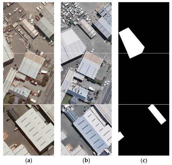
Figure 6.
Two-phase images and change information of the WHU building dataset. (a) image1; (b) image2; (c) label.
The LEVIR-CD building change-detection data set was proposed by the team of Beijing University of Aeronautics and Astronautics. The data time span is from 2002 to 2018, and the experimental area is 20 different areas in Texas. Due to the large time span of the data and many seasonal changes, there are many “pseudo changes” caused by natural growth factors in the data set. The original image was also cut to 256 × 256 size and then we obtained 10,192 pairs of samples. To keep the positive and negative sample ratio of 4:1, we extracted all the positive samples (4538 pairs) and randomly selected a suitable number of negative samples (1135 pairs) from the negative samples.
We also enhanced the data, randomly transformed all samples by rotating 90°, 180° and 270° clockwise, and obtained 11,376 samples in total. Finally, we divided the samples into a training set, verification set and test set according to 7:2:1 randomly, and 7942 training samples, 2269 verification samples and 1135 test samples were obtained. The basic information of the data is shown in Table 2, and the clipped partial sample data are shown in Figure 7.
Table 2.
LEVIR-CD building dataset basic information.
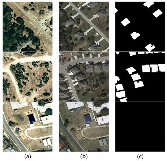
Figure 7.
Two-phase images and change information of the LEVIR-CD building dataset. (a) image1; (b) image2; (c) label.
3.2. Accuracy Test
In this section, we performed ablation experiments on ICD networks. We conducted experiments on the WHU dataset and the LEVIR-CD dataset on the network using gradient points without secondary feature extraction (Gradient_No_Res), with the network using solid points with secondary feature extraction (Disc_Res) and the network using gradient points with secondary feature extraction (Gradient_Res), and we evaluated the accuracy indicators under 0, 1, 5 and 10 clicks, in the experiment.
The original dataset contains three folders A, B and Label, which correspond to the phase 1 image, phase 2 image and real building change label (Figure 8a,b,e). On this basis, we added two new folders, C and D, corresponding to the positive and negative clicks (Figure 8c,d). Before starting training, we should initialize the clicks, which means generating the corresponding single channel pure white label. In the training process, each new generation updates the positive and negative clicks of the current samples. When the clicks of all training samples are updated, the next round of training will start.
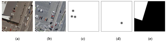
Figure 8.
Training sample. (a) Image1; (b) Image2; (c) Positive Clicks; (d) Negative Clicks; (e) Label.
Based on the PyTorch deep-learning framework, we deployed all training data and code in one unit with the Ubuntu16.04.4 system server. The server processor is a Core i7-8700k, the memory is 32 G, the video memory is GTX2080Ti-12G, and it has four NVIDIA 2080Ti-GPU independent graphics cards. In the model training process, we set the learning rate as 1 × 10⁻⁴ and the iteration generations to 200. After training, we tested the model accuracy with 0, 1, 5, and 10 positive and negative clicks. During the test, we select the center of the first 10 areas to be corrected as the click location. If the number of areas to be corrected is less than 10, we will return to the first largest area to be corrected and continue to select points after all centers of the areas to be corrected are selected. According to the principle of minimizing the distance between the latest point and the selected point in the area and all boundary points, the remaining points were selected in the remaining areas. The experimental results are shown in Table 3.
Table 3.
Accuracy table of the model.
According to the experimental results, the accuracy of Gradient_Res should be better than Gradient_No_Res and Disc_Res; as the number of clicks increases, F1-score of Gradient_Res on WHU and LEVIR-CD can increase by 4.3% and 4.2%, respectively, which proves that the prediction-result accuracy can be greatly improved through user interaction. For the click-correction range, the value of the click-correction range becomes more stable with the increase in the number of clicks. When the number of clicks reaches 10, the positive click-correction ranges (CR_positive) of Gradient_Res in WHU and LEVIR-CD are 0.779 and 0.815, respectively, indicating that an average positive click can fill 80% of the detection holes in the corresponding area, while the corresponding negative click correction ranges (CR_negative) are 0.546 and 0.655, respectively, indicating that an average negative click can eliminate 50% of the false detection areas.
The difference between Disc_Res and Gradient_Res is that the clicks used by the former are solid points, while those used by the latter are gradient points. According to the experimental results, Gradient_Res’s click correction ability is better than that of Disc_Res. The F1-score of Disc_Res on WHU and LEVIR-CD can be increased by 3.4% and 2.9%, respectively, compared with Gradient_Res, which should be 0.9% and 1.3% lower, respectively. In terms of the click-correction range, the positive click-correction ranges of Disc_Res in WHU and LEVIR-CD are 0.876 and 0.835, respectively, which are higher than Gradient_Res of 0.097 and 0.020, and the negative click correction ranges are 0.507 and 0.532, respectively, which are lower than Gradient_Res of 0.039 and 0.123. Although there is little difference in various indicators between the two methods, in the process of actual use, the click-correction capability of Disc_Res is not as stable as that of Gradient_Res. Whether it is a positive click or a negative click, the impact range of its clicks is greater than that of Gradient_Res (Figure 9b1–b6,c1–c6. Therefore, in the case of the same radius, the correction ability of the gradient point is higher than that of the solid point.
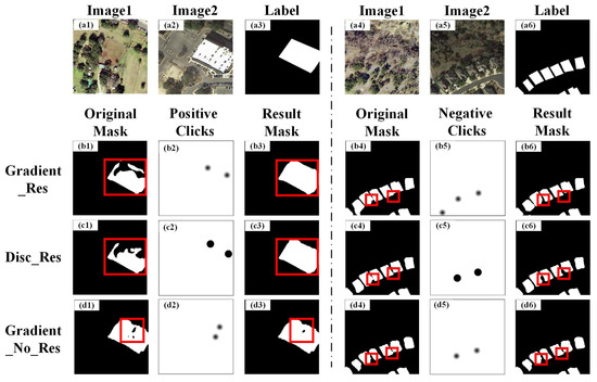
Figure 9.
Comparison of correction effects of different models. (a1–a6) original samples; (b1–b6) results of Gradient_Res; (c1–c6) results of Disc_Res; (d1–d6) results of Gradient_No_Res.
Structurally, Gradient_Res is better than Gradient_No_Res, and the difference between them is that the former has an extra ResNet feature-extraction operation in the click fusion module. According to the experimental results, Gradient_Res click correction ability is better than that of Gradient_No_Res. The F1-score of Gradient_No_Res on WHU and LEVIR-CD can be increased by 1.4% and 0.9%, respectively, compared with Gradient_Res, which should be 2.9% and 3.3% lower, respectively. In terms of click correction range: The positive click correction ranges of Gradient_No_res in WHU and LEVIR-CD are 0.352 and 0.495, respectively, which are lower than Gradient_Res of 0.427 and 0.320, and the negative click correction ranges are 0.355 and 0.476, respectively, which are lower than Gradient_Res of 0.191 and 0.179. They have a very clear gap between F1-score and click correction range. In the process of actual use, the correction effect of Gradient_No_Res is far less than that of Gradient_Res; specifically, the range of positive click correction is narrowed and inaccurate (Figure 9d3), and the negative click correction is incomplete (Figure 9d6). However, after adding secondary feature extraction, its correction ability will greatly improve; specifically, the positive clicks can automatically complete the area to be corrected ((Figure 9b3), and the negative clicks can effectively separate the adhesive patches (Figure 9b6). Therefore, the secondary feature extraction in the click fusion module can improve the correction ability of clicks.
In summary, Gradient_Res, which uses gradient points and secondary feature extraction, is the optimal network structure, and users can effectively modify the area by adding positive and negative clicks. The test results of the LEVIR-CD dataset under the ICD network are shown in Figure 10, in which all changed areas are marked with a red box, and the original mask, result mask and label represent the original forecast result, click correction result and actual change label, respectively. Figure 10a6–c6) show the effect of using positive clicks to make the houses not fully predicted obtain the full prediction, which shows that a positive click can effectively fill in the prediction vacancy; Figure 10b6,d6 show the effect of partial negative-click segmentation on the glued houses. It can be seen that the negative clicks in the figure can segment the gaps between the houses without affecting the shape of the houses.
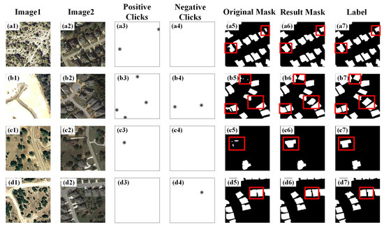
Figure 10.
Correction results of ICD on the LEVIR-CD dataset. Column Image1 (a1–d1): phase 1 image; Column Image2 (a2–d2): phase 2 image; Column Positive Clicks (a3–d3): positive clicks; Column Negative Clicks (a4–d4): negative clicks; Column Original Mask (a5–d5): original predict results; Column Result Mask (a6–d6): the correction results; Column Label (a7–d7): ground truth.
4. Discussion
4.1. Discussion of the Experiment
We proposed an interactive change-detection network (ICD) based on deep learning. By adding click weights to the distance layer of the change-detection network, the network can accept the intervention of external interaction to achieve the effect of revising the original prediction results. It can improve the prediction result accuracy and reduce the human-intervention workload. Compared with the original change-detection network, users only need to add a small number of positive and negative clicks to obtain higher accuracy results than the original network.
In terms of network structure, we designed the click-fusion module with reference to the interactive segmentation network of a single-stream structure, fused the positive and negative clicks at the distance map of the dual stream change detection network, and compared the difference caused by whether to carry out secondary feature extraction after the fusion of clicks. According to the experimental results, the click-fusion module for secondary feature extraction has better correction ability, which indicates that more feature-extraction operations on the feature layer can improve the correction effect of clicks.
In terms of the click-drawing method, we improved the existing click-drawing method and tested it on the open source dataset WHU and the homemade dataset LEVIR-CD. According to the experimental results, in the case of the same radius, the overall correction effect of the gradient point is better than that of the solid point, and the correction stability of the former is higher than that of the latter.
We used the optimal model structure to test WHU and LEVIR-CD. The results show that the F1-score of the model on WHU and LEVIR-CD can be increased by 4.3% and 4.2%, respectively. The positive and negative click-correction ranges are 0.779 and 0.815 and 0.546 and 0.655, respectively. This shows that adding clicks can effectively improve the detection accuracy and correct the area to be corrected. In addition, the positive click-correction amplitude of the two models is higher than the negative click-correction amplitude, so the correction ability of the positive clicks is stronger than that of the negative clicks. Moreover, the area to be corrected of the negative clicks is usually located at the boundary of the actual change area, which makes the negative click-correction more difficult because it needs to account for the elimination of the error area and the maintenance of the change area boundary.
4.2. Application Scenario
The interactive change-detection network we proposed can be applied in many scenarios, such as rapid correction of natural-resource monitoring results and the efficient production of change-detection samples. In actual business scenarios such as natural-resource monitoring, due to the wide range of monitoring patches and large color difference between pictures, it is difficult for the conventional change-detection results to meet the application standards. It often includes false detection and missing detection of map spots. If it is to be put into use, it must be corrected manually. Manual correction requires operations such as filling the hole in the vector patch, delineating the wrong boundary, segmenting the connected patch and eliminating the wrong patch (Figure 11), which means that the whole correction process requires considerable manpower and time. However, interactive change detection can effectively simplify these processes, and the user only needs to add clicks to the error areas to complete the correction. Therefore, the interactive change-detection network can effectively improve the resulting correction efficiency of the change detection method based on deep learning in the actual natural resource monitoring business. In addition, to quickly correct the detection results, the interactive change-detection network can also be used in change-detection sample production. We can click to correct the change detection results with minor defects, and the corrected results can be used as new change-detection samples.
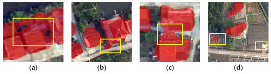
Figure 11.
Example of the error patch. (a) the hole; (b) wrong boundary; (c) the connected patch; (d) wrong patch.
4.3. Deficiency and Future Improvement Direction
Although ICD can effectively correct erroneous patterns, it still has some problems. For example, when a user adds clicks in an incorrect place, it may have a negative impact on the detection result. As shown in Figure 12b1–b3, when the user adds positive clicks to the unchanged area, a small-scale circular misjudgment will occur at the corresponding position. While in Figure 12c1–c3, if the user adds negative clicks to the changed area, it is difficult to make error correction, which indicates that the influence of positive clicks is greater than that of negative clicks. In addition, when the correction area is located at the patch boundary, if the click position is not accurate, the boundary shape will be affected (Figure 12b4–b6 shows the accurate correction results, while Figure 12c4–c6 shows the inaccurate correction results). Therefore, the correction effect of ICD depends on the judgment of the user to a certain extent. If the click position is inaccurate or incorrect, it is difficult for the network to correct the detection result.
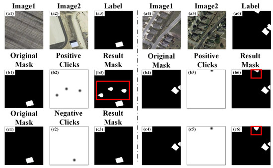
Figure 12.
Wrong clicks example. (a1–a6) original samples; (b1–b3) correction results of wrong positive clicks; (c1–c3) correction results of wrong negative clicks; (b4–b6) the accurate correction results; (c4–c6) the inaccurate correction results.
In addition, during the test, the machine will automatically take the centroid of the area to be corrected as the center of the clicks. In the actual operation, the user will select the click according to the actual situation, that is, there may be more accurate clicks in some areas. Therefore, the correction effect of the selected points is often better than the effect of the points selected by the machine, and the correction accuracy in actual use is higher than the test result.
Therefore, we will have two improvement directions in future research. One is to optimize the click performance so that it will not affect the original correct-detection results when clicking at the wrong position. The other is to optimize the existing point selection algorithm so that it can select the correction position more accurately and the results calculated in the model accuracy verification are closer to the actual situation when the point is manually selected.
Author Contributions
Conceptualization, Z.J. and W.C.; methodology, Z.J. and X.Z.; software, X.Z.; validation, Z.J. and W.C.; formal analysis, Z.S.; investigation, Z.S.; resources, C.W.; data curation, C.W.; writing—original draft preparation, Z.J.; writing—review and editing, W.C.; visualization, X.Z.; supervision, Z.S.; project administration, C.W.; funding acquisition, C.W. All authors have read and agreed to the published version of the manuscript.
Funding
This research was supported by National Natural Science Foundation of China under Grant 42201504 and 41471318, Open Foundation of Key Lab of Virtual Geographic Environment of Ministry of Education (No. 2021VGE02).
Data Availability Statement
Not applicable.
Conflicts of Interest
The authors declare no conflict of interest.
References
- Ashbindu, S. Review Article Digital Change Detection Techniques Using Remotely-Sensed Data. Int. J. Remote Sens. 1988, 10, 989–1003. [Google Scholar]
- Haigang, S.; Wenqing, F.; Wenzhuo, L.; Kaimin, S.; Chuan, X. Review of Change Detection Methods for Muti-temporal Rempte Sensing Imagery. Geomat. Inf. Sci. Wuhan Univ. 2018, 43, 1885–1898. [Google Scholar]
- Hussain, M.; Chen, D.; Cheng, A.; Wei, H.; Stanley, D. Change Detection from Remotely Sensed Images:From Pixel-Based to Object-Based Approaches. ISPRS J. Photogramm. Remote Sens. 2013, 80, 91–106. [Google Scholar] [CrossRef]
- Karantzalos, K. Recent Advances on 2D and 3D Change Detection in Urban Environments from Remote Sensing Data. Comput. Approaches Urban Environ. 2014, 13, 237–272. [Google Scholar]
- Lu, D.; Mausel, P.; Brondizio, E.; Moran, E. Change Detection Techniques. Int. J. Remote Sens. 2004, 25, 2365–2401. [Google Scholar] [CrossRef]
- Zhigao, Y.; Qianqing, Q.; Qifeng, Z. Change Detection in High Spatial Resolution Images Based on Support Vector Machine. In Proceedings of the IEEE International Conference on Geoscience and Remote Sensing Symposium 2006, Denver, CO, USA, 31 July–4 August 2006. [Google Scholar] [CrossRef]
- Huang, X.; Xie, Y.; Wei, J.; Fu, M.; Lv, L.L.; Zhang, L.L. Automatic Recognition of Desertification Information Based on the Pattern of Change Detection-CART Decision Tree. J. Catastrophol. 2017, 31, 36–42. [Google Scholar]
- Seo, D.K.; Yong, H.K.; Yang, D.E.; Park, W.Y.; Park, H.C. Generation of Radiometric, Phenological Normalized Image Based on Random Forest Regression for Change Detection. Remote Sens. 2017, 9, 1163. [Google Scholar] [CrossRef]
- Lu, J.; Ming, L.; Peng, Z.; Yan, W.; Huahui, Z. SAR Image Change Detection Based on Multiple Kernel k-Means Clustering with Local-Neighborhood Information. IEEE Geosci. Remote Sens. Lett. 2016, 13, 856–860. [Google Scholar]
- Lv, H.; Lu, H.; Mou, I. Learning a Transferable Change Rule from a Recurrent Neural Network for Land Cover Change Detection. Remote Sens. 2016, 8, 506. [Google Scholar]
- Lu, J.; Ming, L.; Peng, Z.; Wu, Y. SAR Image Change Detection Based on Correlation Kernel and Multistage Extreme Learning Machine. IEEE Trans. Geosci. Remote Sens. 2016, 54, 5993–6006. [Google Scholar]
- Guo, C.; Yazhou, L.; Yanfeng, S. Automatic Change Detection in Remote Sensing Images Using Level Set Method with Neighborhood Constraints. J. Appl. Remote Sens. 2014, 8, 83–678. [Google Scholar]
- Ming, H.; Hua, Z.; WenZhong, S.; Kazhong, D. Unsupervised Change Detection Using Fuzzy-Means and MRF from Remotely Sensed Images. Remote Sens. Lett. 2013, 4, 1185–1194. [Google Scholar]
- Licun, Z.; Guo, C.; Yupeng, L.; Yanfeng, S. Change Detection Based on Conditional Random Field with Region Connection Constraints in High-Resolution Remote Sensing Images. IEEE J. Sel. Top. Appl. Earth Obs. Remote Sens. 2016, 9, 3478–3488. [Google Scholar]
- Khelifi, L.; Mignotte, M. Deep Learning for Change Detection in Remote Sensing Images: Comprehensive Review and Meta-Analysis. IEEE Access 2020, 8, 126385–126400. [Google Scholar] [CrossRef]
- Hao, C.; Zhenwei, S. A Spatial-Temporal Attention-Based Method and a New Dataset for Remote Sensing Image Change Detection. Remote Sens. 2020, 12, 1662. [Google Scholar]
- Jie, C.; Ziyuan, Y.; Li, C.; Jian, P.; Haozhe, H.; Jiawei, Z.; Yu, L.; Haifeng, L. DASNet: Dual attentive fully convolutional siamese networks for change detection of high resolution satellite images. IEEE J. Sel. Top. Appl. Earth Obs. Remote Sens. 2020, 14, 1194–1206. [Google Scholar]
- Ken, S.; Mikiya, S.; Weimin, W. Weakly Supervised Silhouette-based Semantic Scene Change Detection. In Proceedings of the IEEE International Conference on Robotics and Automation (ICRA), Paris, France, 31 May–31 August 2020; pp. 6861–6867. [Google Scholar]
- Mengxi, L.; Qian, S.; Andrea, M.; Da, H.; Xiaoping, L.; Liangpei, Z. Super-resolution-based Change Detection Network with Stacked Attention Module for Images with Different Resolutions. IEEE Trans. Geosci. Remote Sens. 2021, 60, 4403718. [Google Scholar]
- Lin, W.; Haiyan, L. Interactive Segmentation Algorithm for Bio-medicine Image. Comput. Eng. 2010, 36, 208–212. [Google Scholar]
- Wei, H.; Qingwu, H.; Mingyao, A. Interactive Remote Sensing Image Segmentation Based on Multiple Star Prior and Graph Cuts. Remote Sens. Inf. 2016, 31, 19–23. [Google Scholar]
- Sofiiuk, K.; Petrov, I.A.; Konushin, A. Reviving Iterative Training with Mask Guidance for Interactive Segmentation. arXiv 2021. [Google Scholar] [CrossRef]
- Huayue, Z.; Shunli, Z.; Li, Z. Interactive Target Segmentation Algorithm Based on Two-Stage Network. Comput. Eng. 2021, 47, 300–306. [Google Scholar]
- Castrejon, L.; Kundu, K.; Urtasun, R.; Fidler, S. Annotating Object Instances with a Polygon-RNN. In Proceedings of the 2017 IEEE Conference on Computer Vision and Pattern Recognition (CVPR) 2017, Honolulu, HI, USA, 21–26 July 2017. [Google Scholar]
- Sahbi, H.; Deschamps, S.; Stoian, A. Active learning for interactive satellite image change detection. arXiv 2021. [Google Scholar] [CrossRef]
- Hui, R.; Huai, Y.; Pingping, H.; Wen, Y. Interactive Change Detection Using High Resolution Remote Sensing Images Based on Active Learning with Gaussian Processes. ISPRS Ann. Photogramm. Remote Sens. Spat. Inf. Sci. 2016, 3, 141. [Google Scholar]
- Hichri, H.; Bazi, Y.; Alajlan, N.; Malek, S. Interactive Segmentation for Change Detection in Multispectral Remote-Sensing Images. IEEE Geosci. Remote Sens. Lett. 2013, 10, 298–302. [Google Scholar] [CrossRef]
- Saux, B.L.; Randrianarivo, H. Urban Change Detection In SAR Images By Interactive Learning. In Proceedings of the 2013 IEEE International Geoscience and Remote Sensing Symposium, Melbourne, VIC, Australia, 21–26 July 2013. [Google Scholar] [CrossRef]
- Mahadevan, S.; Voigtlaender, P.; Leibe, B. Iteratively trained interactive segmentation. arXiv 2018. [Google Scholar] [CrossRef]
- Junhao, L.; Yunchao, W.; Wei, X.; Ong, S.-H.; Feng, J. Regional Interactive Image Segmentation Networks. In Proceedings of the 2017 IEEE International Conference on Computer Vision (ICCV) 2017, Venice, Italy, 22–29 October 2017; pp. 2746–2754. [Google Scholar] [CrossRef]
- Honglin, W.; Lichen, J.; Fangfang, X. Interactive Segmentation Technique and Decision-level Fusion Based Change Detection for SAR Images. Acta Geod. Cart. Sin. 2012, 41, 74–80. [Google Scholar]
- Xinying, H.; Jiazhong, W.; Chenxia, S.; Chang, S. Edge detection method based on mathematical morphology and canny algorithm. J. Comput. Appl. 2008, 8, 477–478. [Google Scholar]
- Shunping, J.; Shiqing, W. Building extraction via convolutional neural networks from an open remote sensing building dataset. Acta Geod. Cartogr. Sin. 2019, 48, 448–459. [Google Scholar]
Publisher’s Note: MDPI stays neutral with regard to jurisdictional claims in published maps and institutional affiliations. |
© 2022 by the authors. Licensee MDPI, Basel, Switzerland. This article is an open access article distributed under the terms and conditions of the Creative Commons Attribution (CC BY) license (https://creativecommons.org/licenses/by/4.0/).