Using Multiple Scale Space-Time Patterns to Determine the Number of Replicates and Burn-In Periods in Spatially Explicit Agent-Based Modeling of Vector-Borne Disease Transmission

Abstract

(1) Background: The stochastic nature of agent-based models (ABMs) may be responsible for the variability of simulated outputs. Multiple simulation runs (i.e., replicates) need to be performed to have enough sample size for hypothesis testing and validating simulations. The simulation outputs in the early-stage of simulations from non-terminating ABMs may be underestimated (or overestimated). To avoid this initialization bias, the simulations need to be run for a burn-in period. This study proposes to use multiple scale space-time patterns to determine the number of required replicates and burn-in periods in spatially explicit ABMs, and develop an indicator for these purposes. (2) Methods: ABMs of vector-borne disease transmission were used as the case study. Particularly, we developed an index, D, which enables to take into consideration a successive coefficient of variance (CV) over replicates and simulation years. The comparison between the number of replicates and the burn-in periods determined by D and those chosen by CV was performed. (3) Results: When only a single pattern was used to determine the number of replicates and the burn-in periods, the results varied depending on the pattern. (4) Conclusions: As multiple scale space-time patterns were used for the purposes, the simulated outputs after the burn-in periods with a proper number of replicates would well reproduce multiple patterns of phenomena. The outputs may also be more useful for hypothesis testing and validation.

1. Introduction

Spatially explicit agent-based models (ABMs) have been widely used across disciplines, such as land-use science [1,2], public health [3,4], ecology [5], economics, criminology [6,7], and so forth. In ABMs, the phenomena of interest are described and captured through the interactions of heterogeneous agents and their environments. Due to the limited sources of observations for developing ABMs [8], models often include uncertain assumptions and parameters. The stochastic nature of ABMs may be responsible for generating simulated outputs with variability [9]. Therefore, to understand a spatiotemporal phenomenon being modeled, the stochastic nature needs to be figured out through uncertainty quantification [10,11,12]. Also, this uncertainty quantification requires many simulation runs [13]. In addition, one realization from such stochastic simulation models may not be representative; it may be extreme. Therefore, multiple simulation runs need to be performed to have proper sample sizes for hypothesis testing (e.g., what-if scenario analysis) and validating simulation models [14,15,16]. The number of simulation runs varies according to the researchers, and it often ranges from ten to 100 [17,18,19,20,21,22]. The question about how many simulation runs are required still needs to be answered.

In addition, initialization bias [16,23] is also a significant issue in non-terminating simulation modeling. This bias results in simulation outputs at early-stages of simulations that may overestimate or underestimate the outcomes. The simulation runs are usually performed until the models reach equilibrium (i.e., steady-state [24]) in simulation outputs [14,25], which are called burn-in periods (or warm-up periods). The long-term simulation may be needed to avoid obtaining the data during such initial transient periods. The temporally dependent effects on input factors embedded in the model have been quantitatively measured using the variance-based global sensitivity analysis [26]. Although the values of each parameter are swept via a Monte Carlo simulation, the effects of input parameters become stable after a certain period of time. This may imply that the values of parameters do not affect the nature of non-terminating simulation models.

Since spatially explicit ABMs represent and simulate spatiotemporal phenomena, the simulated outputs should be similar to the observations from the real-world for the validation purpose [27,28]. Following pattern-oriented modeling protocol [29], the simulation outputs can be summarized at multiple space-time scales [30]. Particularly, ABMs of communicable disease transmission simulate spatiotemporal patterns of disease outbreaks. Although the disease outbreaks take place at different places and times in each single simulation, the general patterns would be detected. There are spatiotemporally clustered patterns in influenza [31] and dengue outbreaks Aldstadt [32]. Therefore, the interesting question would be how many simulation runs can successively describe the spatiotemporal patterns of modeling outputs. In addition, the simulated outcomes would vary depending on the variations in initial conditions and stochastic components embedded in the model [33]. Therefore, the question about how the spatiotemporal patterns of simulated outcomes can be incorporated for determining the required number of replicates and the burn-in period need to be answered.

To address these issues, this study proposes the use of multiple scale space-time patterns. Specifically, we develop an indicator for determining the number of simulation runs, and the burn-in period. As a benchmark, the results of the proposed indicator are compared to the coefficient of variation (CV), which is the frequently used indicator to determine the number of replicates [15]. A spatially explicit ABM of dengue virus (DENV) transmission [30] was used as the case study. DENV is a mosquito-borne disease, which is transmitted primarily by Aedes mosquitoes. In the ABM, DENV transmission occurs through interactions between human and female mosquito agents. The ABM is a non-terminating susceptible, infectious, or recovered model. This study does not focus on measuring how closely the model reproduces the observed patterns of DENV outbreaks, but highlights the usefulness of multiple space-time patterns to determine the number of replicates and the length of simulation runs. Our research questions are as follows: (1) how the multiple scale spacetime patterns as the simulated outcomes of ABMs of DENV outbreaks can be summarized? (2) to what extent such patterns would vary according to the number of replicates and the burn-in periods, (3) how the multiple scale spacetime patterns can be incorporated for determining the number of replicates, and the burn-in periods?

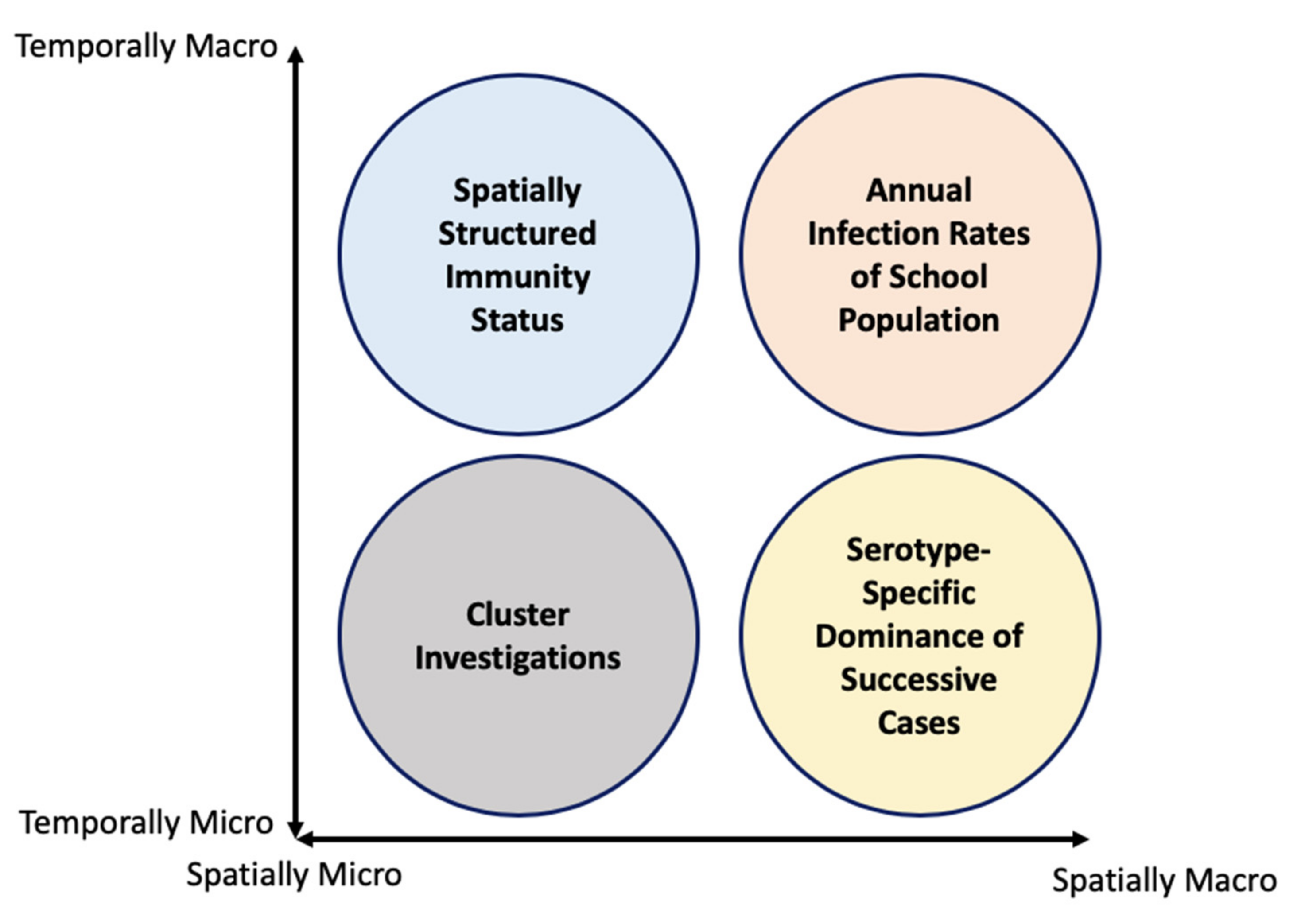
2. Multiple Scale Spacetime Patterns

Spatially explicit ABMs produce events with spatial location and time of occurrence so that simulation outputs can be summarized and described by spatiotemporal patterns. Considering the ABMs are needs to be run multiple times, the spacetime patterns are described as a mean or median value of the simulated outcomes. For example, the average of the total infection cases and the average of the cleaning time are often used for ABMs of infectious disease [4,22,34] and for ABMs of evacuation [35,36,37], respectively. Spatiotemporal patterns also largely depend on space-time scale, which may be divided into four types of patterns [30]. The four types of patterns are as follows: (1) spatially macro and temporally macro scale pattern (e.g., annual rates of disease or crime outbreaks in a city), (2) spatially macro and temporally micro scale pattern (e.g., short-term rates of disease or crime in a city), (3) spatially micro and temporally macro scale pattern (e.g., annual rates of disease or crime outbreaks at a particular place, such as a hospital/school/park), and (4) spatially micro and temporally micro scale pattern (e.g., short-term rates of disease or crime outbreaks in a neighborhood).

In order to determine the number of simulations (i.e., runs) and the burn-in periods in spatially explicit ABMs, we propose the use of multiple scale space-time patterns (Figure 1). The patterns used in this paper include (1) annual infection rates of school population (spatially-macro-temporally-macro scale pattern); (2) serotype-specific dominance of successive cases (spatially-macro-temporally-micro scale pattern); (3) spatially structured immunity status (spatially-micro-temporally-macro scale pattern); and (4) cluster investigations (spatially-micro-temporally-micro scale pattern).

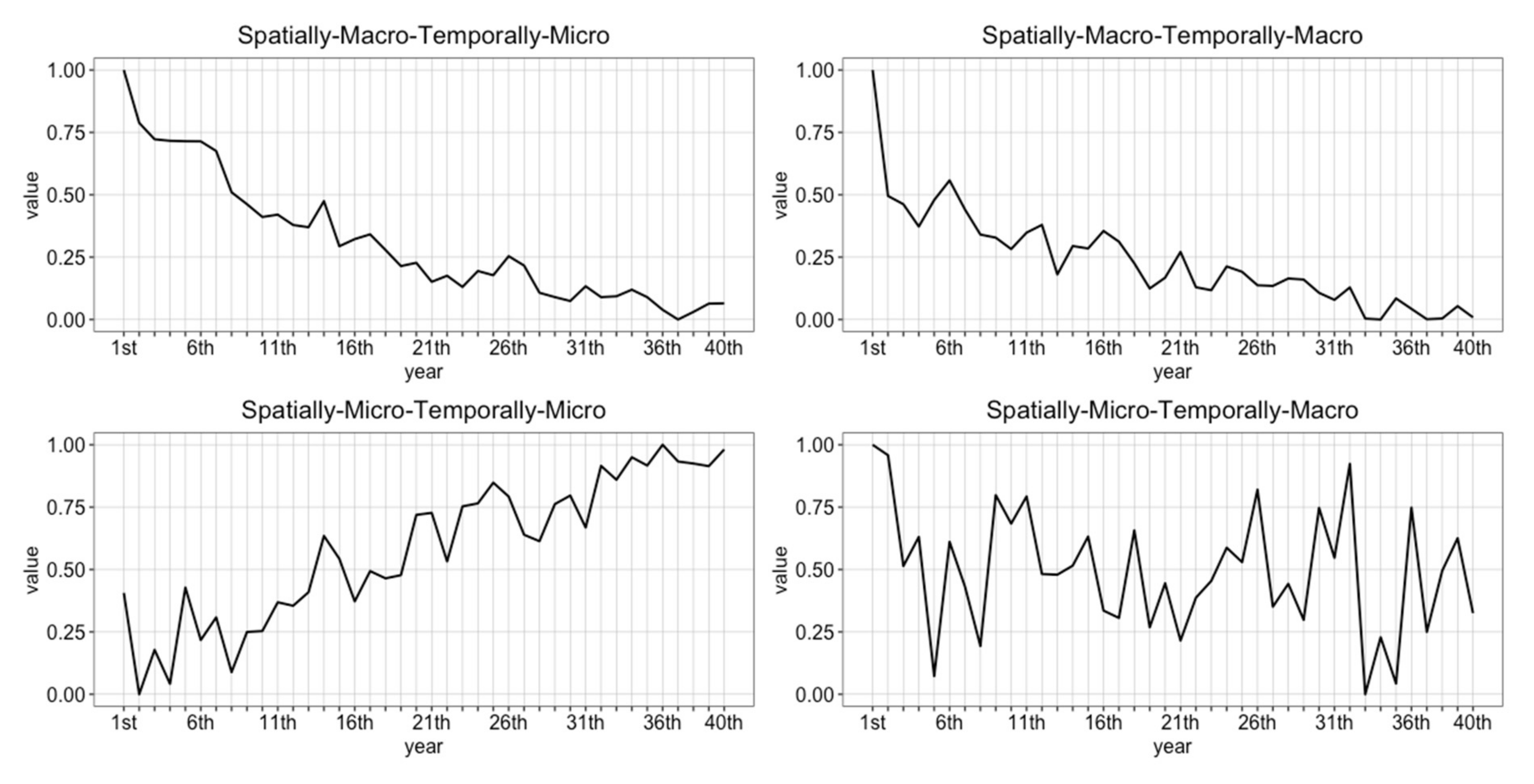
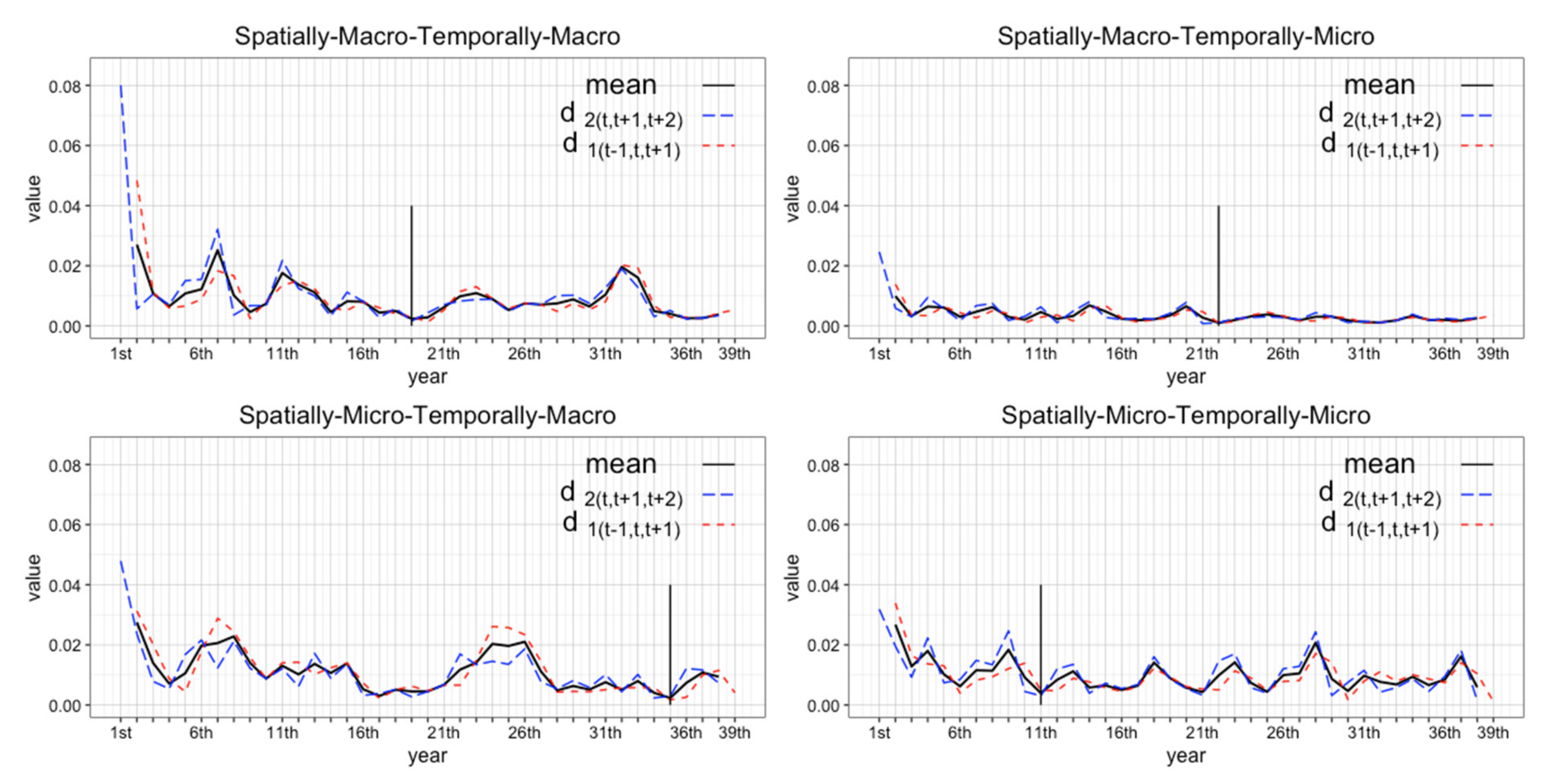
2.1. Spatially-Micro-Temporally-Macro Scale Pattern

In spatially explicit ABMs of disease outbreaks, the infection rates (i.e., total cases per total populations) are often used as a measurement of simulation outputs [34,38]. As a spatially-micro-temporally-macro pattern, annual infection rates at the study area can be used. Particularly, Endy, Chunsuttiwat [39] found about 6% of school population were annually infected by DENV.

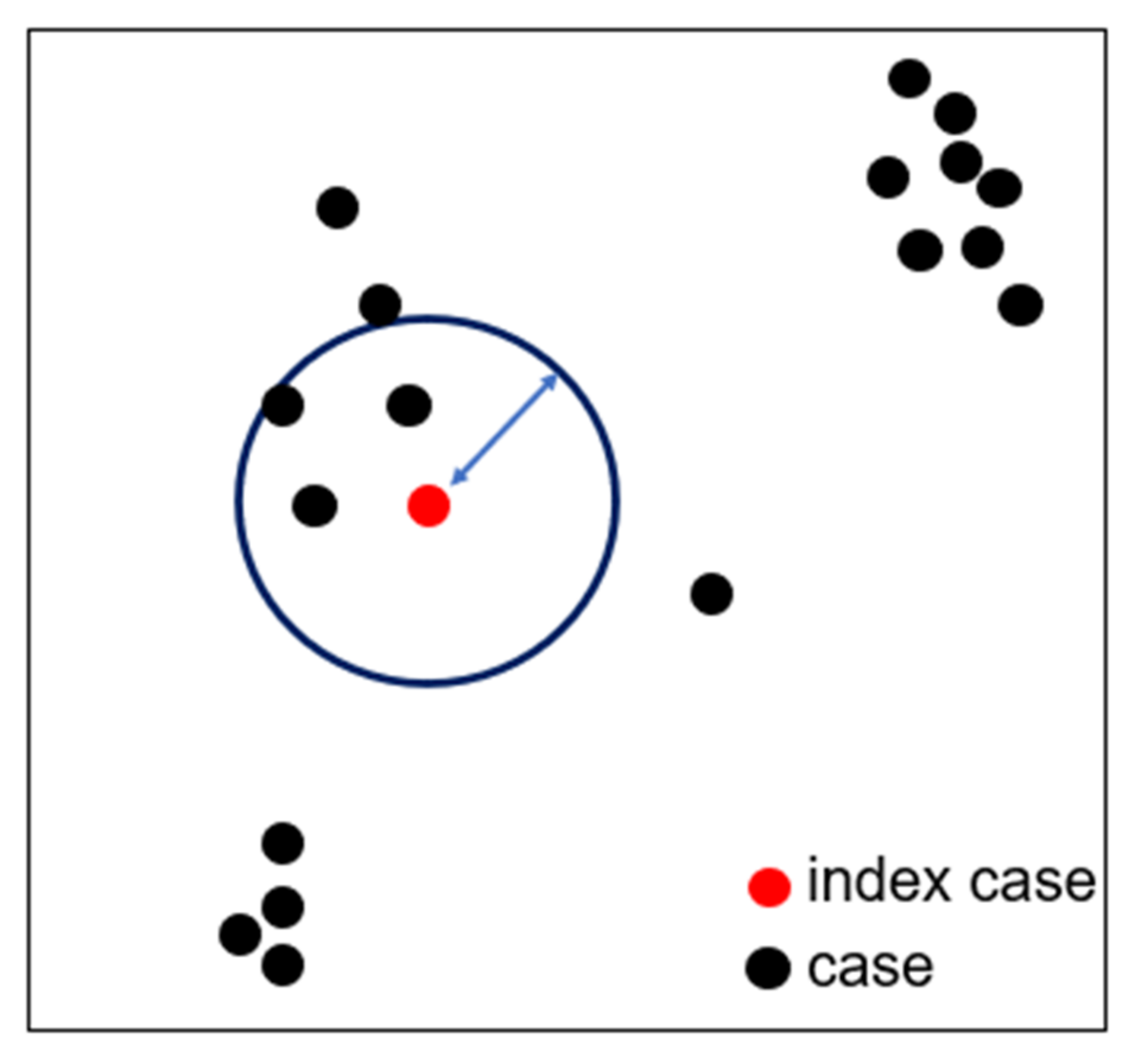
2.2. Spatially-Macro-Temporally-Micro Scale Pattern

In our model, there are two ways a susceptible person may become infected with DENV. First, a person may become infected from DENV introduced from or contracted outside the study area. The second route of infection is through the bite of a mosquito that became infected within the study area. Infections due to local transmission through the mosquito vectors will always have the same serotype. This process results in single serotypes predominating in local areas during a single transmission season (Endy et al., 2002). Therefore, examining the local serotype-dominance during DENV outbreaks would be a pattern of interest [40]. Importantly, when local transmission of DENV is responsible for a majority of infections, temporally successive infections should largely be of the same serotype.

2.3. Spatially-Micro-Temporally-Macro Scale Pattern

Considering there are four serotypes of DENV and that infection confers life-long immunity against the infecting serotype, the immunity status of each serotype in individual human agents should be preserved over time in ABMs of DENV transmission. At the beginning of our simulation, individual agents’ immunity statuses for each of the four serotypes are simulated based on his/her age but are not spatially structured. Considering the focality of dengue transmission, local immunity status should also be spatially structured [30]. Therefore, we used a local immunity structure as a spatially micro and temporally macro pattern to assess whether the model has been properly initialized. Given that mosquito’s movement radius was defined within 100 m, the spatially structured DENV immunity can be measured within 100 m from the firstly chosen case for this measurement (Figure 2).

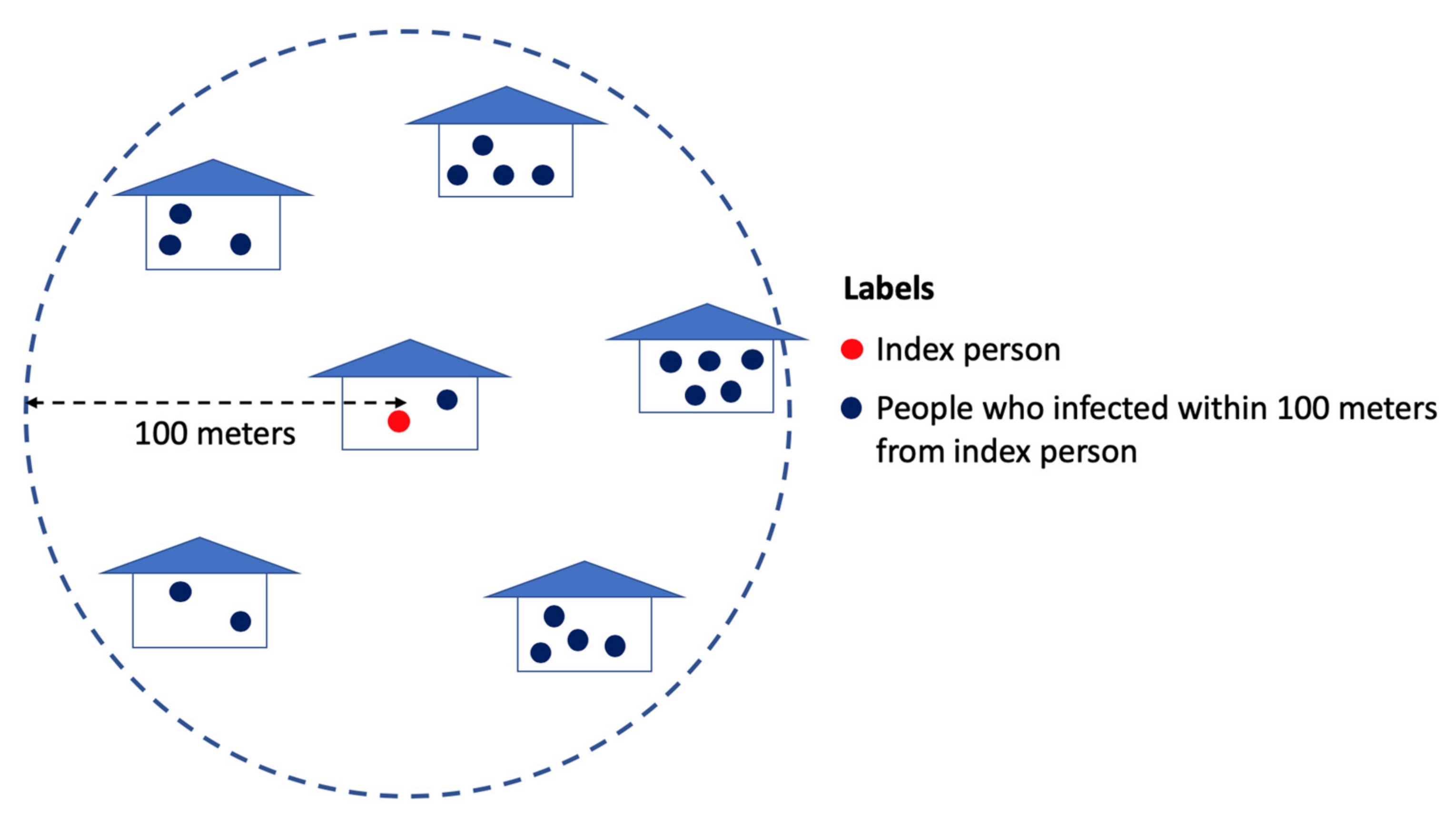
2.4. Spatially-Micro-Temporally-Micro Scale Pattern

The spatiotemporal patterns of DENV outbreaks at a micro spatial and micro temporal scale will be examining cluster investigations [41] (Figure 3). Cluster investigations have been summarized by measuring the infection rates of residents at each distance interval (i.e., at the same household, <0–20, <20–40, <40–60, <60–80, <80–100 m) within the vicinity of a selected dengue case. The cases that occurred in the 3 weeks prior and subsequent 15 days since the index case were included in the cluster investigation. The procedure of the cluster investigations is performed as follows: (1) select a random dengue cases (i.e., index case), (2) find other cases within time period (i.e., −21 to 15 days) at each distance interval, (3) measure the infection rates (i.e., case per people) at each distance interval, and (4) repeat procedure 1–3 50 times. Then, the results from the clustering investigation would show a distance-decay pattern. As a distance from an index case increases, infection rates at distance intervals decrease.

3. Materials and Methods

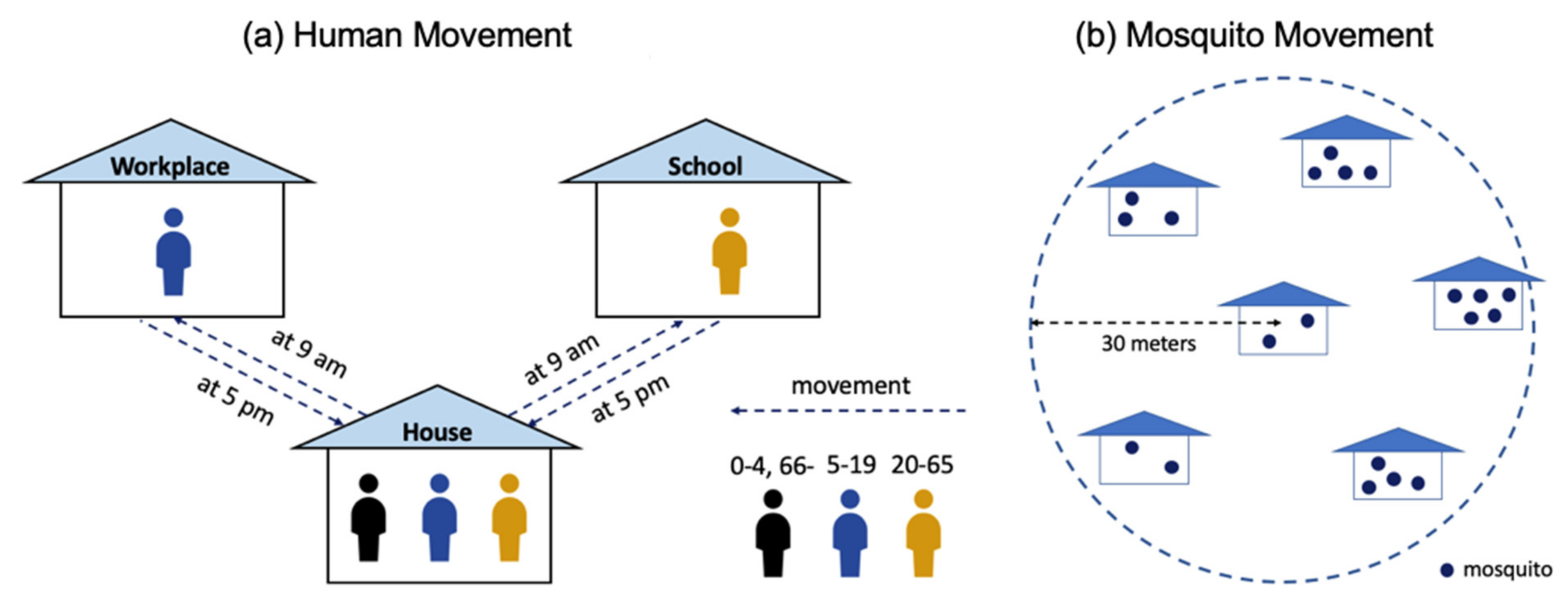
3.1. Agent-Based Model of DENV Transmission

In this paper, we used a spatially explicit ABM of DENV transmission in a part of Kamphaeng Phet province, Thailand as the case study. The validity of this model was tested [30]. The assumptions embedded in the model were quantitatively assessed by comparing the space-time patterns of simulated outcomes and observations at multiple space-time scales. For the details of the model, please find the Overview, Design Concepts and Details (ODD) protocol [42], provided in Kang and Aldstadt [30]. This model is also available at the AnyLogic cloud (https://cloud.anylogic.com/model/64d09b7f-fcd6-4b04-af26-834a26be569d?mode=SETTINGS) accessed on 17 July 2021. The model consists of three components: (1) individual human agents, (2) mosquito agents, and (3) an environment. In the model, four distinct serotypes of DENV were included to account for the nature of DENV transmission. A person with exposure to one serotype of DENV will develop a lifelong immunity to that serotype [43]. There also exists short-term cross-protection for 120 days [34]. After 120 days, individual human become at risk of becoming infected by other serotypes that they have not been previously exposed to [44].

In the model, human and infectious female mosquito agents interact each other through mosquito’s bites. DENV is transmitted between human hosts and mosquito vectors, as follows: (1) a susceptible human is bitten by an infectious female mosquito, and (2) a susceptible female mosquito bites an infectious human. We assumed age-specific movements of human agents. Individuals commute to their schools (ages 5 to 19) or workplace (ages 20 to 64) in the morning (9:00 a.m.) and they come back to their home in the evening (5:00 p.m.). Therefore, they are co-located with their classmates and co-workers in daytime (9:00 a.m.–5:00 p.m.), and they are also co-located with their household members during the rest of time (5:00 p.m.–9:00 a.m.). The rest of the population stays at their home all day. The infected human stays at his/her home until he/she is recovered (Figure 4a).

The mosquitoes travel to nearby places (within 30 m) with a 0.15 probability [34]. If there are multiple places within 30 m, mosquitoes travel to a random place among the multiple places. The mosquitoes also can travel to a randomly selected place with a 0.01 probability [34]. (Figure 4b). The number of mosquitoes is assumed to be identical to every building. Due to the hot and humid summer in Thailand, the number of mosquitoes is seasonally variable (i.e., 42 in June and two in February). Mosquitoes bite humans at four-time intervals (08–13 h, 13–18 h, 18–24 h, and 00–08 h) with probabilities of 0.08, 0.76, 0.13, and 0.03, respectively. The mosquito’s hazard rates are determined based on its age [45,46,47].

To answer the research questions regarding the temporal change in multiple scale space-time patterns requires an adequate number of simulation runs (replicates) over a long duration. Therefore, we ran 1000 replicates for 40 years. The patterns of modeling outputs were measured for the four space-time scales, as illustrated in Figure 1.

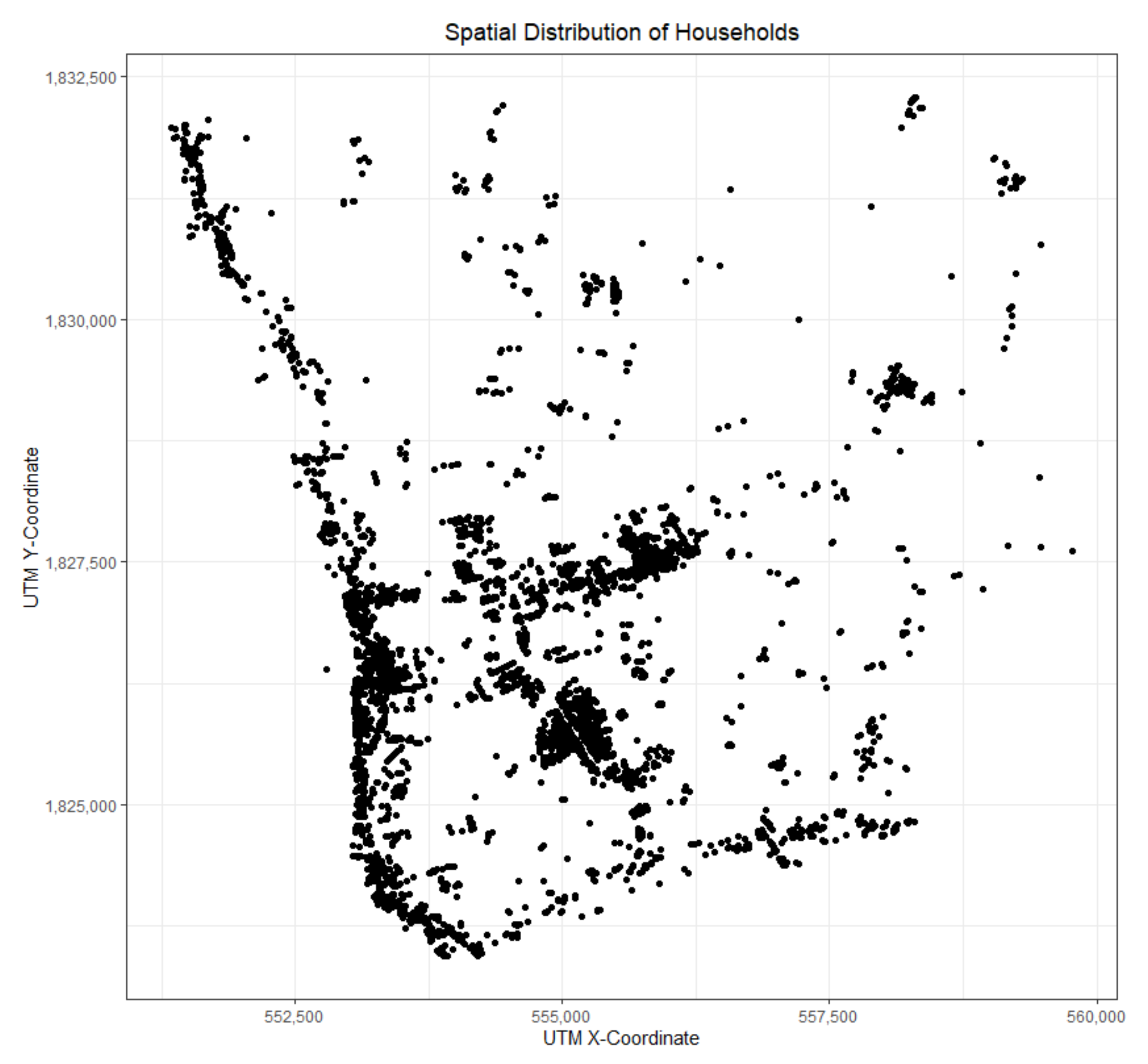
3.2. Study Area and Data

A portion of Kamphaeng Phet province in Thailand was taken as a study area. In the study area, 3680 houses, 186 workplaces, and eight schools are located (Figure 5). The locations (i.e., x and y coordinates) of houses, workplaces and schools were identified from Lidar data. The composition of households was obtained from Microdata on households in 2009 [48]. The demographic changes (i.e., birth rates and death/out-migration rates) were calculated based on population data provided by the Department of Provincial Administration (DOPA), Ministry of Interior, Thailand.

3.3. Measures

3.3.1. Multiple Scale Space-Time Patterns

As described in Section 2, we explored four space-time patterns, as follows: (1) infection rates of school population; (2) similarity of serotypes of successive cases; (3) local immunity status; and (4) cluster investigations.

An infection rate for school population as a spatially-macro-temporally-macro scale pattern was measured in the following (1):

$$P_1=\frac{total infection cases of school popuation}{school population}\times 100$$

(1)

To measure a spatially-macro-temporally-micro scale pattern, we examined the diversity in serotypes of the successive dengue cases. Specifically, a case is randomly chosen, and the cases occurred before 3 weeks and following 15 days were also selected. Then, the Shannon diversity index (H) was measured over the selected cases. The Shannon diversity index is a commonly used measure to characterize the diversity of species in a community [49]. In regard to the spatially-macro-temporally-micro scale pattern, the index provides a measure of the commonness of serotypes during dengue virus outbreaks and ranges from zero to one. The higher values indicate more diversity in serotypes of dengue cases, while the lower values show less diversity serotypes of dengue cases. In this study, the proportion of serotype, j relative to the total number of serotype (p_j) is calculated. R denotes to the number of serotypes (i.e., four) (2).

$$H_i=-{{\displaystyle \sum }}_{j=1}^R{p}_j\ln p_j$$

(2)

Using the calculated value through Equation (2), the diversity in serotypes of the successive dengue cases were measured. Following Yoon, Getis [41], 50 clusters were selected and the Shannon diversity index over each cluster was measured. Then, the Shannon diversity index were averaged by the number of cluster, n (3). In this case, n is equal to 50.

$$P_2=\frac{{{\displaystyle \sum }}_{i=1}^n{H}_i}{n}$$

(3)

A spatially-micro-temporally-macro scale pattern were calculated through the similarity of immunity statuses against the four DENV serotypes in geographic clusters. Under natural conditions, immune statuses of individuals living near one another will be similar due to exposure to previous outbreaks. First, 50 clusters are randomly chosen mirroring the approach of Yoon, Getis [41]. We measured the variance of immunity status against serotypes of individual human agents within 100 m of a selected infection.

$$P_3=\frac{{{\displaystyle \sum }}_{i=1}^n{V}_i}{n}$$

(4)

where n denotes the number of clusters (50) and Vi denotes the variance in immunity statuses by serotypes in the local population.

For cluster investigation as a spatially-micro-temporally-micro-scale pattern, we simplified the measurement in the following. Given a mosquito’s relative short distant movement (i.e., <100 m) [47] and mosquito’s extrinsic incubation periods (i.e., 11 days) [34], spatiotemporal patterns can be captured by calculating the infection rates within 100 m. The pattern was measured using the following equation:

$$P_4=\frac{{{\displaystyle \sum }}_{i=1}^n{r}_i}{n}$$

(5)

where, r_i denotes the DENV infection rates (%) in cluster i, cluster i includes the cases occurring prior to three weeks and following 15 days after a randomly chosen index case within 100 m, and n denotes the number of clusters (50).

3.3.2. Coefficient of Variance

One common practice to quantify and summarize patterns of simulated outcomes is statistical description, such as means, or variances (or standard deviation). The determination of the number of replicates may depend on the stability of the simulated outcomes [15]. To acquire the meaningful results from simulation, the mean and variance over simulated runs may need to be used. In this paper, we used CV of each space-time pattern, which is a statistical measure of the dispersion of data. In other words, the standard deviation and mean values refer to the standard deviation and the mean values of each P₁, P₂, P₃, and P₄, which were calculated from Equations (1) and (3)–(5).

$$CV=\frac{standard deviation}{mean}$$

(6)

CV helps to identify whether the significant variance in simulated outcomes exist, which helps to identify the standard error of the mean [15]. It has been also suggested as a measure or criterion to determine the needed number of replicates. Specifically, it is to find a certain point at which CV does not change while increasing the number of replicates [33].

3.3.3. Incorporating Successive Coefficient of Variance

To determine the number of replicates, CV of the patterns with a certain number of replicates would not be significantly different from that of a greater number of replicates. Therefore, we developed two indicators (i.e., d₁(p,t) and d₂(p,t)), as follows:

$$d_{1\left(p,t\right)}=\frac{abs\left|C{V}_{p, t-1}-C{V}_{p,t}\left| + abs\right|C{V}_{p,t+1}-C{V}_{p,t}\right|}{2}$$

(7)

$$d_{2\left(p,t\right)}=\frac{abs\left|C{V}_{p, t}-C{V}_{p,t+1}\left| + abs\right|C{V}_{p,t}-C{V}_{p,t+2}\right|}{2}$$

(8)

where p denotes a space-time pattern and t denotes the number of replicates.

To lower the computational costs, the number of replicates was determined with an increase in increments of 25. The number of replicates is [25, 50, 75, …, 950, 975, 1000]. d₁(p,t) shows whether CV of a pattern with a certain number of replicates would be similar to those of both a smaller and larger number of replicates, while d₂(p,t) indicates whether CV of a pattern with a certain number of replicates is similar to larger number of replicates. In other words, a smaller value of d₁(p,t) means the CV of a pattern, p, with the number of replicates, t has a smaller difference to the values of CV with the numbers of replicates, t − 1, and t + 1. A smaller d₂(p,t) means the CV of a pattern, p, with the number of replicates, t has a smaller difference compared to the values of CV with the numbers of replicates, t + 1, and t + 2.

Following pattern-oriented modeling [29,50], the modeling outputs need to well reproduce multiple patterns at multiple space-time scales [30]. Thus, d₁ and d₂ of each pattern are normalized and averaged in the following:

$$D_1={\displaystyle \sum }_p^{4}normal\_d_{1\left(p,t\right)}$$

(9)

$$D_2={\displaystyle \sum }_p^{4}normal\_d_{2\left(p,t\right)}$$

(10)

$$D=\frac{(D_1+D_2)}{2}$$

(11)

D is the average of D₁ and D₂. The minimum value of D indicates an optimal (or near-optimal) number of replicates, which does not have significant differences of CV of multiple space-time patterns.

To determine the burn-in period of the simulation, we also used the same measurements (d₁(p,t) and d₂(p,t)). In the measurements, t denotes simulation lengths, which is [1st, 2nd, 3rd, 4th, …, 37th, 38th, 39th, 40th]. The patterns for CV are the results of the number of replicates that would be determined by the above measurements.

4. Results

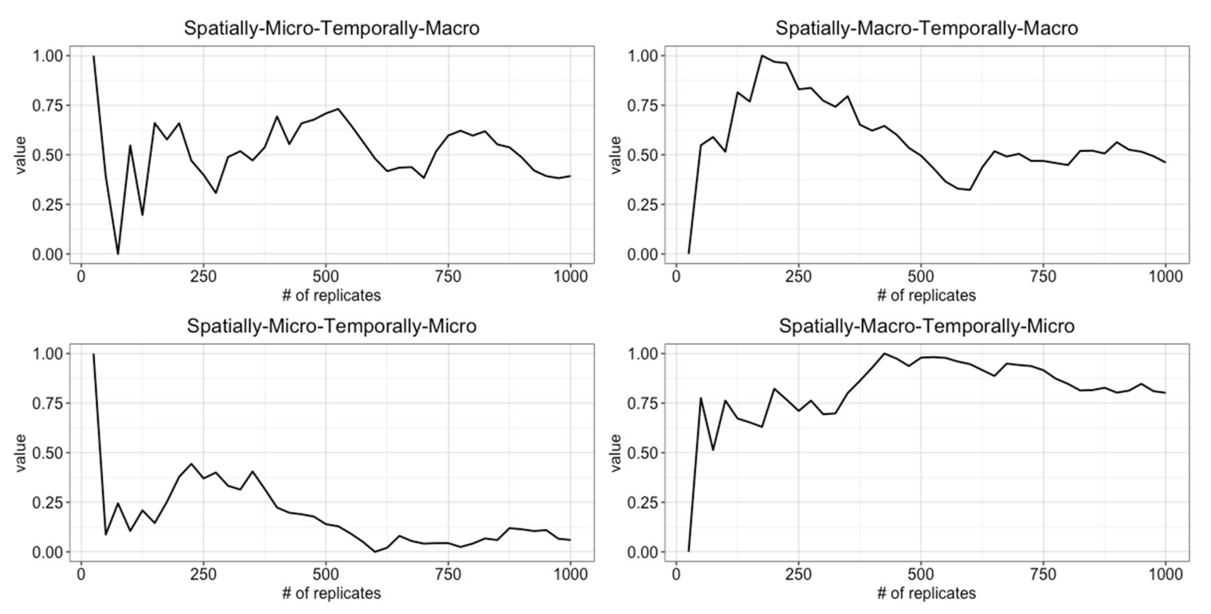
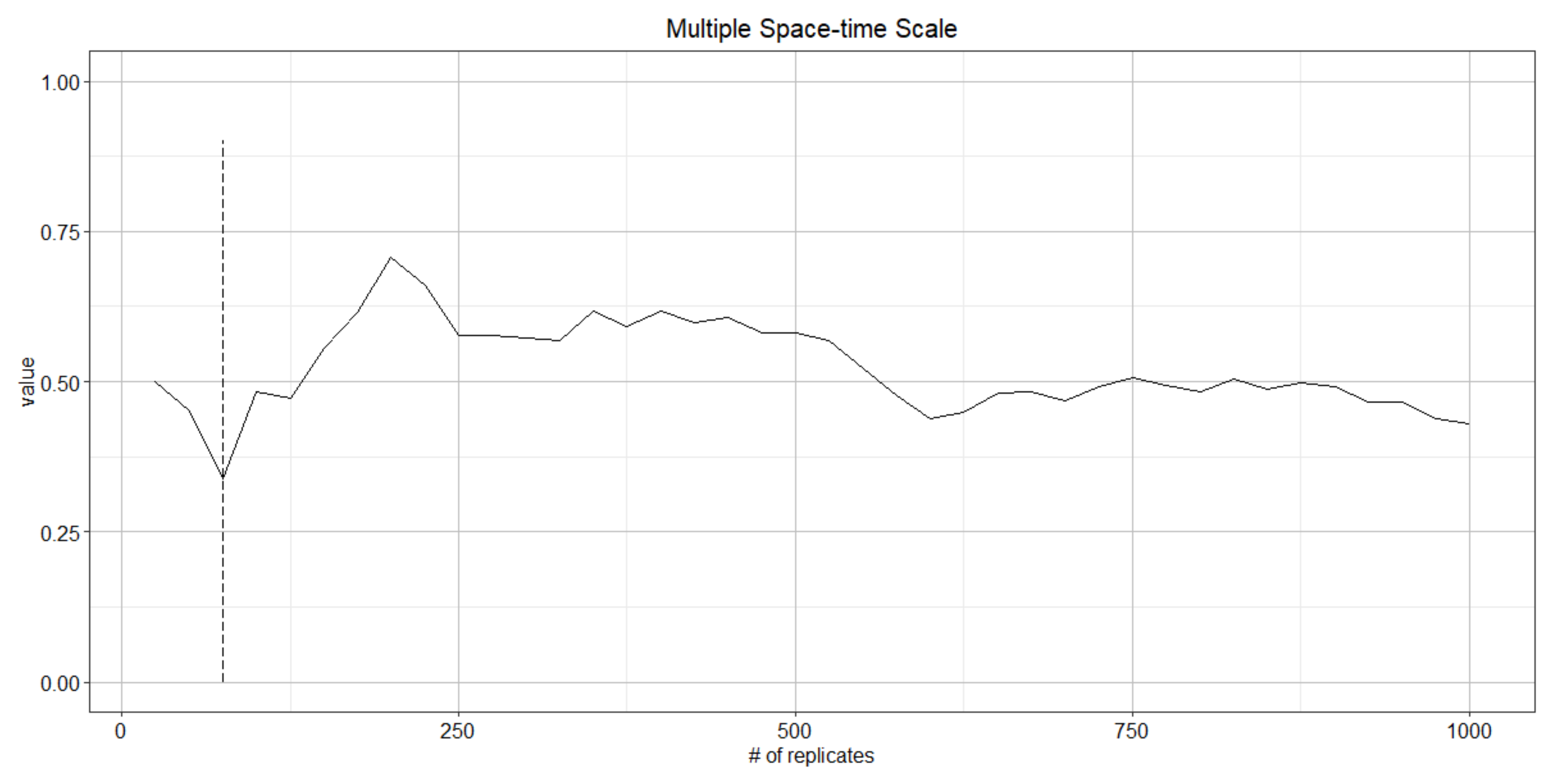
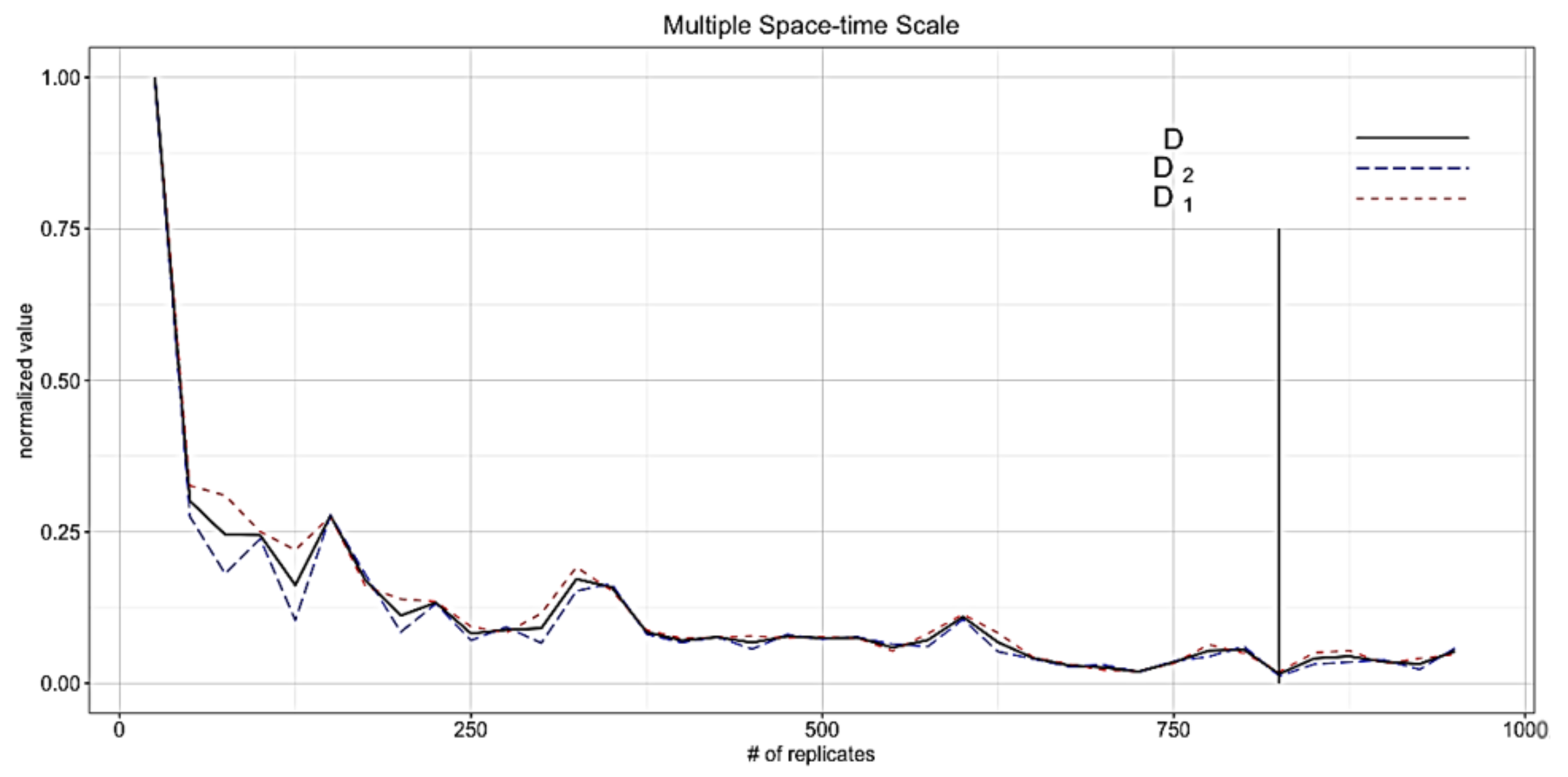
4.1. Determining the Number of Replicates

As we described in Section 3, we measured the D to determine the number of replicates necessary for hypothesis testing. For this, the simulated outcomes of the first simulation year were used and measured at multiple space-time scales, including spatially-macro-temporally-macro pattern (annual infection rates of school population), spatially-macro-temporally-micro pattern (serotype-specific dominance of successive cases), spatially-micro-temporally-macro pattern (spatially structured immunity status) and spatially-micro-temporally-micro pattern (cluster investigation). We also used the normalized CV as a benchmark to compare the results from using D.

The normalized CV indicates how stable simulated outcomes are for a number of simulation runs. The lowest normalized CV indicates that simulated outcomes with a specific number of replicates have the least variability in simulated outcomes. Given that many simulation runs may avoid sampling bias of simulation results, simulated outcomes having less variability help to properly interpret simulated outcomes.

Figure 6 provides the change in the normalized CV over the number of replicates. X- and Y-axis refer to the number of replicates and the value of normalized CV for each pattern. The results can be explained in the following. First, the outputs of spatially-micro-temporally-macro pattern were not stable while increasing the number of replicates. Second, after about 200 replicates, the outputs of spatially-macro-temporally-macro pattern became less variable. Third, the variability in outputs of spatially-micro-temporally-micro patterns became smaller as the number of replicates increased. Last, the variability in outputs of spatially-macro-temporally-micro pattern became more larger with more replicates.

Since the normalized CV at four spatio-temporal scales became the least at the different number of replicates, it is challenging to determine how many simulation runs are needed to well capture the reference patterns of real-world phenomena. In addition, we also found that the averaged value over CVs may not be helpful for this purpose. As shown in Figure 7, the average of normalized CVs was the least variable at 75 replicates. However, 75 replicates may not be good choices as the number of replicates. Simulated outcomes were more stable after 575 replicates, and then they became less variable and stable. Therefore, other measurement to determine the number of replicates is needed. This result is also consistent to that Lee, Filatova [15] that CV may not be stable while increasing the number of replicates.

Instead of using CV, we calculated D to determine the minimum number of replicates. For this, the modeling outputs of the first simulation year were used and measured at multiple space-time scales, including spatially-macro-temporally-macro pattern (annual infection rates of school population), spatially-macro-temporally-micro pattern (serotype-specific dominance of successive cases), spatially-micro-temporally-macro pattern (spatially structured immunity status) and spatially-micro-temporally-micro pattern (cluster investigation). Figure 8 illustrates d₁(p,t) and d₂(p,t) at each scale. Given that d₁ and d₂ are measured based on the successive values of CV, they have some variability with the small number of replicates. Particularly, the normalized CV of spatially-macro-temporally-macro pattern and spatially-macro-temporally-micro pattern are larger at beginning (Figure 6). In each panel in Figure 8, vertical lines represent the number of replicates that have the minimum value of averages of d₁(p,t) and d₂(p,t).

Based on D, the number of replicates can be determined. D is an average of D₁ (average of d₁ of all patterns) and D₂ (average of d₂ of all patterns). Since D values take into consideration the successive values of CV, it helps to avoid the ambiguity that occurred when using only CV. Compared to the CVs (Figure 6), it is found that the D₁ and D₂ become noticeably stable as the number of replicates increases.

Figure 9 illustrates the changes of D₁, D₂, and D over the number of replicates. Since D₁ and D₂ of each pattern oscillate with the small number of replicates, D has some variability with the small number of replicates. Based on D, 825 simulation runs are the proper number of replicates that are able to robustly represent the multiple space-time patterns. As Figure 8, the required number of replicates would vary depending on the spatiotemporal patterns chosen in measurements. It is noted that value D could adjust a certain pattern that the variability of output may not reach to the stability.

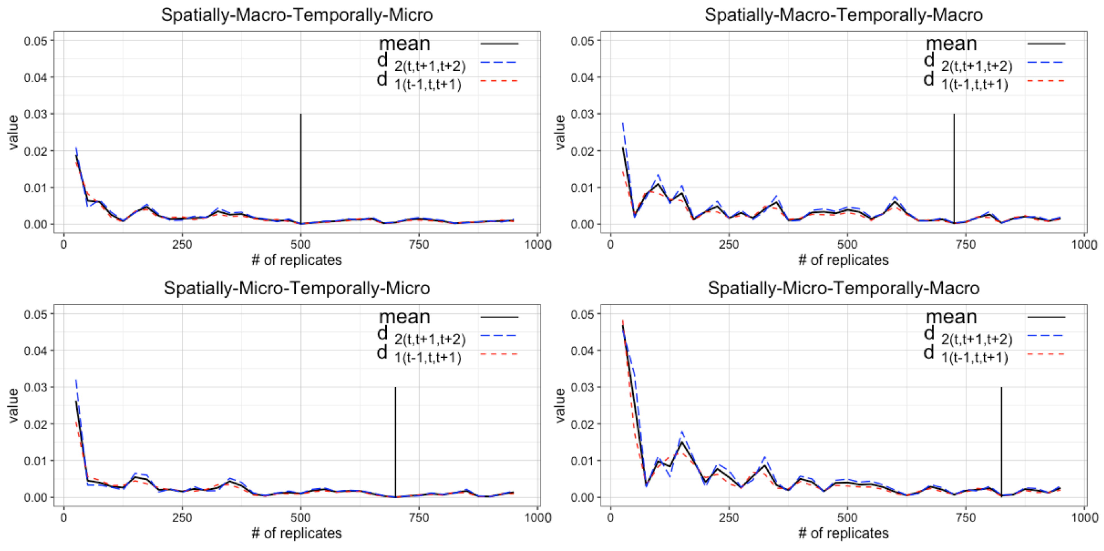
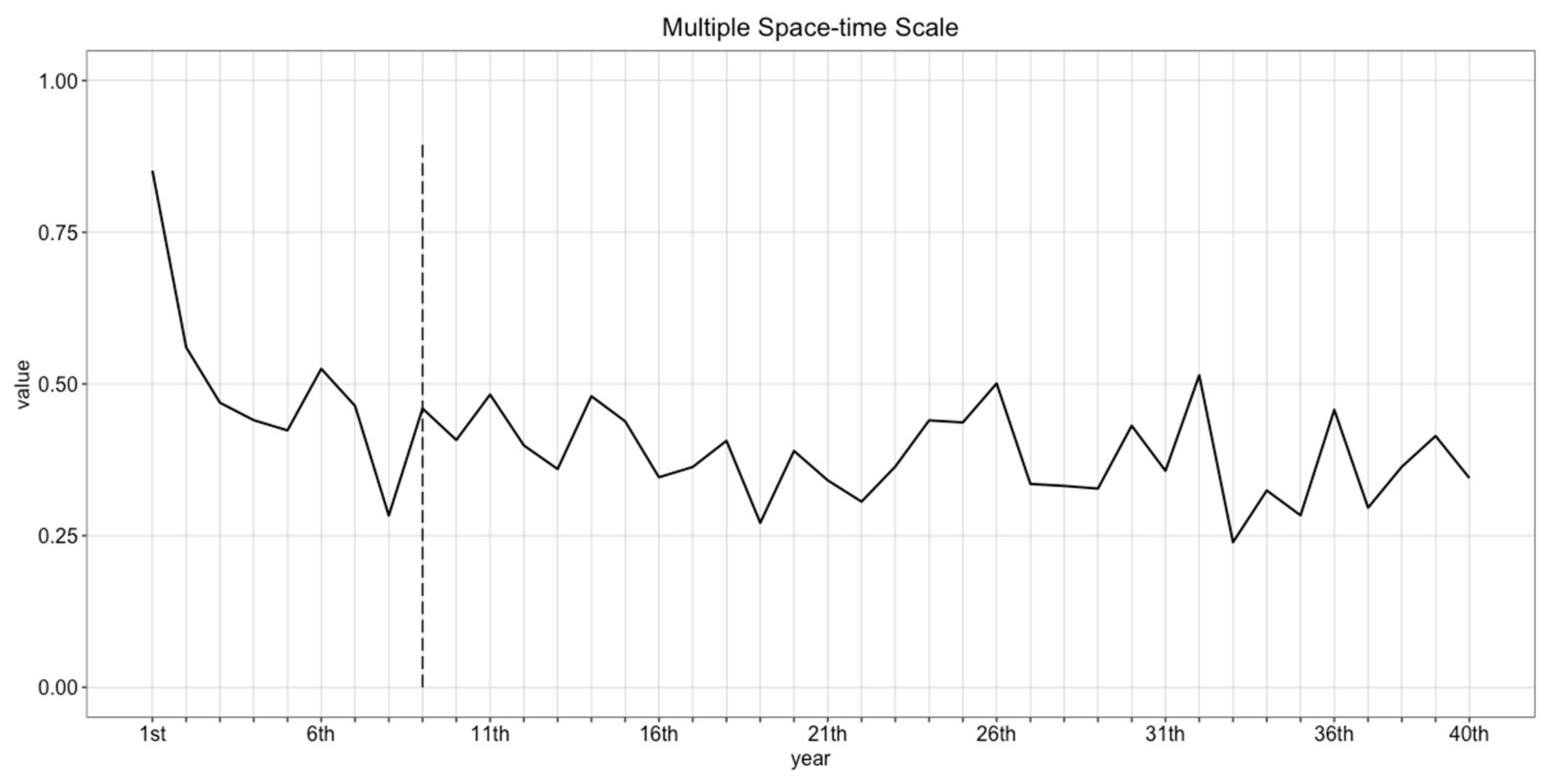
4.2. Determining Burn-in Period

To determine burn-in period, we measured the normalized CVs of each pattern with 250 replicates as chosen through the average of the normalized CVs. Generally, over simulation year, spatially-macro-temporally-macro and spatially-macro-temporally-micro patterns became less variable, spatially-micro-temporally-macro pattern remained at the same level of variability, and spatially-micro-temporally-micro patterns were more variable as simulation years increased (Figure 10).

Simply using the average of normalized CVs indicates that simulated outcomes after 9th simulation year became relatively stable. However, it may also be problematic. After 32th simulation year, the simulated outcomes became flexible again (Figure 11).

To avoid such issues, D at multiple space-time scales was also measured to determine the burn-in periods (Figure 12). As the required number of replicates was determined as 825, simulated outputs with 825 replicates were used. In each panel in Figure 12, vertical lines represent the burn-in period that have the minimum value of averages of d₁(p,t) and d₂(p,t).

Figure 13 shows the changes of D₁, D₂, and D by simulation year. Although the values of the normalized CV of each pattern were much fluctuating as shown in Figure 10, d₁ and d₂ of each pattern became less variable over year. This is because, such variabilities of the normalized CV were mitigated in d₁ and d₂ while considering successive CV. Based on D, the burn-in period of this spatially explicit ABM [30] should be at least 35 simulation years. In other words, the modeling outputs after the 35th year will robustly represent the multiple scale space-time patterns.

5. Conclusions

ABMs have inevitable issues associated with their stochastic nature and initialization bias. Due to the stochastic nature of ABMs, multiple simulation runs need to be performed. Also, the simulation outputs from early-stages of non-terminating ABMs may not properly represent the phenomena being modeled. These issues may be resolved by running a large number of replicates for a long duration, but this may result in unnecessary computational effort. In addition, the simulated outputs are often represented at multiple space-time patterns. For the purposes of hypothesis testing, evaluation, and validation, multiple scale space-time patterns need to be measured. In this regard, it is of importance to incorporate the multiple scale space-time patterns to determine the number of replicates and the burn-in periods in spatially explicit ABMs. Therefore, this paper proposes an indicator (D) to determine the number of replicates and the bun-in periods for the ABMs, through an experimental approach.

To fully consider the tendency of simulation outputs, we used CV (standard deviation divided by the mean), and compared the simulation runs and burn-in period determined by simply using CV. As we found, the CVs would not be a good choice to determine the simulation runs and burn-in periods. This result can support the argument from [15], which is the CV may have a variability due to a small mean value. As an alternative, our proposed indicator, D(p,t) can be used to determine the proper number of replicates and the burn-in periods. We found the usefulness of multiple scale space-time patterns in determining the number of replicates as well as the burn-in periods. when taking a particular space-time pattern into account, the results vary according to the pattern chosen in measurements.

Compared to the typical methods that qualitatively determine the number of replicates and the burn-in periods, the method proposed in this study would be helpful to quantitively determine them. We do not argue that our findings (i.e., 825 replicates and 35 years of burn-in period) are correct to other models. The number of replicates and the burn-in period may be different from our findings, according to the model’s components (e.g., parameter, agent’s behaviors). Rather, we highlight the usefulness of multiple scale space-time patterns for these purposes. Then, the modeling outputs after the burn-in periods with a proper number of replicates, determined by the methods proposed in this study, would reproduce reasonable patterns at multiple space-time scales. Model replication can play a vital role in validation and verification, and determining the number of replicates necessary for valid comparisons is an important step in this process [14].

An approach we proposed here can be applied into other ABMs. For example, simulated outcomes from ABMs for crime [6] are summarized at three spatial scales (e.g., city-wide, household, and individual level). Another example is ABMs for animal movement. Animal movement patterns can be characterized with quantitative metrics at multiple scales (individual-level, location-based, etc.) [51]. Given that the spatiotemporal patterns for infectious disease spreads are often captured though an ABM approach, our indicator can be useful for this example as well. However, it is noted that our proposed indicator would not be applicable to the ABMs whose simulated outcome may not reach to equilibrium [52]. Given that determining the proper number of simulation runs is not a simple task in the field of agent-based modeling [15], our work provides a useful way to choose the number of simulation runs.

Using multiple scale space-time patterns in model calibration would be an apparent next step. To date, the only available observations for our study area are annual infection rates for the school population [39] as the spatially-macro-temporally-macro pattern and the cluster investigations of [41] as the spatially-micro-temporally-micro pattern. Thus, comparing modeling outputs to the observed data to determine the number of replicates and the burn-in periods would be helpful for model tuning. An associated research avenue will be measuring and quantifying the relative value of patterns measured at different spatiotemporal scales for discerning useful models. Then, it is possible to adjust the current indicator (i.e., simply averaging all values from each spatiotemporal patterns), taking into account the relative importance of each pattern on replicating the real-world of being modeled.

References

1. Ligmann-Zielinska, A. Spatially-explicit sensitivity analysis of an agent-based model of land use change. Int. J. Geogr. Inf. Sci. 2013, 27, 1764–1781. [Google Scholar] [CrossRef]
2. An, L.; Linderman, M.; Qi, J.; Shortridge, A.; Liu, J. Exploring Complexity in a Human–Environment System: An Agent-Based Spatial Model for Multidisciplinary and Multiscale Integration. Ann. Assoc. Am. Geogr. 2005, 95, 54–79. [Google Scholar] [CrossRef]
3. Mao, L. Modeling triple-diffusions of infectious diseases, information, and preventive behaviors through a metropolitan social network—An agent-based simulation. Appl. Geogr. 2014, 50, 31–39. [Google Scholar] [CrossRef] [PubMed]
4. Crooks, A.T.; Hailegiorgis, A.B. An agent-based modeling approach applied to the spread of cholera. Environ. Model. Softw. 2014, 62, 164–177. [Google Scholar] [CrossRef]
5. Boyd, R.; Roy, S.; Sibly, R.; Thorpe, R.; Hyder, K. A general approach to incorporating spatial and temporal variation in individual-based models of fish populations with application to Atlantic mackerel. Ecol. Model. 2018, 382, 9–17. [Google Scholar] [CrossRef] [Green Version]
6. Malleson, N.; Birkin, M. Analysis of crime patterns through the integration of an agent-based model and a population microsimulation. Comput. Environ. Urban Syst. 2012, 36, 551–561. [Google Scholar] [CrossRef]
7. Malleson, N.; Heppenstall, A.; See, L. Crime reduction through simulation: An agent-based model of burglary. Comput. Environ. Urban Syst. 2010, 34, 236–250. [Google Scholar] [CrossRef]
8. Crooks, A.; Castle, C.; Batty, M. Key challenges in agent-based modelling for geo-spatial simulation. Comput. Environ. Urban Syst. 2008, 32, 417–430. [Google Scholar] [CrossRef] [Green Version]
9. Rahmandad, H.; Sterman, J. Heterogeneity and network structure in the dynamics of diffusion: Comparing agent-based and differential equation models. Manag. Sci. 2008, 54, 998–1014. [Google Scholar] [CrossRef] [Green Version]
10. Kang, J.-Y.; Aldstadt, J.; Vandewalle, R.; Yin, D.; Wang, S. A CyberGIS Approach to Spatiotemporally Explicit Uncertainty and Global Sensitivity Analysis for Agent-Based Modeling of Vector-Borne Disease Transmission. Ann. Am. Assoc. Geogr. 2020, 110, 1855–1873. [Google Scholar] [CrossRef]
11. Ligmann-Zielinska, A.; Kramer, D.B.; Cheruvelil, K.S.; Soranno, P.A. Using uncertainty and sensitivity analyses in socioecological agent-based models to improve their analytical performance and policy relevance. PLoS ONE 2014, 9, e109779. [Google Scholar] [CrossRef]
12. Ligmann-Zielinska, A.; Jankowski, P. Spatially-explicit integrated uncertainty and sensitivity analysis of criteria weights in multicriteria land suitability evaluation. Environ. Model. Softw. 2014, 57, 235–247. [Google Scholar] [CrossRef]
13. Tang, W.; Jia, M. Global sensitivity analysis of a large agent-based model of spatial opinion exchange: A heterogeneous multi-GPU acceleration approach. Ann. Assoc. Am. Geogr. 2014, 104, 485–509. [Google Scholar] [CrossRef]
14. Fachada, N.; Lopes, V.V.; Martins, R.C.; Rosa, A.C. Model-independent comparison of simulation output. Simul. Model. Pract. Theory 2017, 72, 131–149. [Google Scholar] [CrossRef] [Green Version]
15. Lee, J.-S.; Filatova, T.; Ligmann-Zielinska, A.; Hassani-Mahmooei, B.; Stonedahl, F.; Lorscheid, I.; Voinov, A.; Polhill, G.; Sun, Z.; Parker, D.C. The complexities of agent-based modeling output analysis. J. Artif. Soc. Soc. Simul. 2015, 18, 4. [Google Scholar] [CrossRef]
16. Kelton, W.D. Statistical analysis of simulation output. In Proceedings of the 29th Conference on Winter Simulation, Atlanta, GA, USA, 7–10 December 1997. [Google Scholar]
17. Calisti, R.; Proietti, P.; Marchini, A. Promoting Sustainable Food Consumption: An Agent-Based Model About Outcomes of Small Shop Openings. J. Artif. Soc. Soc. Simul. 2019, 22, 2. [Google Scholar] [CrossRef]
18. Hailegiorgis, A.; Crooks, A.; Cioffi-Revilla, C. An agent-based model of rural households’ adaptation to climate change. J. Artif. Soc. Soc. Simul. 2018, 21, 4. [Google Scholar] [CrossRef] [Green Version]
19. Reinhardt, O.; Hilton, J.; Warnke, T.; Bijak, J.; Uhrmacher, A.M. Streamlining simulation experiments with agent-based models in demography. J. Artif. Soc. Soc. Simul. 2018, 21, 9. [Google Scholar] [CrossRef] [Green Version]
20. Dubbelboer, J.; Nikolic, I.; Jenkins, K.; Hall, J. An agent-based model of flood risk and insurance. J. Artif. Soc. Soc. Simul. 2017, 20. [Google Scholar] [CrossRef]
21. Moglia, M.; Podkalicka, A.; McGregor, J. An agent-based model of residential energy efficiency adoption. J. Artif. Soc. Soc. Simul. 2018, 21. [Google Scholar] [CrossRef]
22. Gharakhanlou, N.M.; Hooshangi, N.; Helbich, M. A Spatial Agent-Based Model to Assess the Spread of Malaria in Relation to Anti-Malaria Interventions in Southeast Iran. ISPRS Int. J. Geo-Inf. 2020, 9, 549. [Google Scholar] [CrossRef]
23. Sanchez, S.M. Output modeling: Abc’s of output analysis. In Proceedings of the 33nd Conference on Winter Simulation, WSC 2001, Arlington, VA, USA, 9–12 December 2001; IEEE Computer Society: Washington, DC, USA, 2001. [Google Scholar]
24. Law, A.M. Statistical analysis of simulation output data: The practical state of the art. In Proceedings of the 2015 Winter Simulation Conference (WSC), Orlando, FL, USA, 14–18 December 2015. [Google Scholar]
25. Garcia, R.; Rummel, P.; Hauser, J. Validating agent-based marketing models through conjoint analysis. J. Bus. Res. 2007, 60, 848–857. [Google Scholar] [CrossRef]
26. Kang, J.-Y.; Aldstadt, J. Using multiple scale space-time patterns in variance-based global sensitivity analysis for spatially explicit agent-based models. Comput. Environ. Urban Syst. 2019, 75, 170–183. [Google Scholar] [CrossRef]
27. Windrum, P.; Fagiolo, G.; Moneta, A. Empirical validation of agent-based models: Alternatives and prospects. J. Artif. Soc. Soc. Simul. 2007, 10, 8. [Google Scholar]
28. Brown, D.; Page, S.; Riolo, R.; Zellner, M.; Rand, W. Path dependence and the validation of agent-based spatial models of land use. Int. J. Geogr. Inf. Sci. 2005, 19, 153–174. [Google Scholar] [CrossRef] [Green Version]
29. Grimm, V.; Revilla, E.; Berger, U.; Jeltsch, F.; Mooij, W.M.; Railsback, S.F.; Thulke, H.-H.; Weiner, J.; Wiegand, T.; Deangelis, D.L. Pattern-oriented modeling of agent-based complex systems: Lessons from ecology. Science 2005, 310, 987–991. [Google Scholar] [CrossRef] [PubMed] [Green Version]
30. Kang, J.-Y.; Aldstadt, J. Using multiple scale spatio-temporal patterns for validating spatially explicit agent-based models. Int. J. Geogr. Inf. Sci. 2019, 33, 193–213. [Google Scholar] [CrossRef]
31. Mao, L.; Bian, L. Agent-based simulation for a dual-diffusion process of influenza and human preventive behavior. Int. J. Geogr. Inf. Sci. 2011, 25, 1371–1388. [Google Scholar] [CrossRef]
32. Aldstadt, J. An incremental Knox test for the determination of the serial interval between successive cases of an infectious disease. Stoch. Environ. Res. Risk Assess. 2007, 21, 487–500. [Google Scholar] [CrossRef]
33. Lorscheid, I.; Heine, B.-O.; Meyer, M. Opening the ‘black box’of simulations: Increased transparency and effective communication through the systematic design of experiments. Comput. Math. Organ. Theory 2012, 18, 22–62. [Google Scholar] [CrossRef]
34. Chao, D.; Halstead, S.B.; Halloran, M.E.; Longini, I.M., Jr. Controlling dengue with vaccines in Thailand. PLoS Negl. Trop. Dis. 2012, 6, e1876. [Google Scholar] [CrossRef] [PubMed] [Green Version]
35. Chen, X.; Meaker, J.W.; Zhan, F.B. Agent-based modeling and analysis of hurricane evacuation procedures for the Florida Keys. Nat. Hazards 2006, 38, 321. [Google Scholar] [CrossRef]
36. Goetz, M.; Zipf, A. Using crowdsourced geodata for agent-based indoor evacuation simulations. ISPRS Int. J. Geo-Inf. 2012, 1, 186–208. [Google Scholar] [CrossRef]
37. Vandewalle, R.; Kang, J.Y.; Yin, D.; Wang, S. Integrating CyberGIS-Jupyter and spatial agent-based modelling to evaluate emergency evacuation time. In Proceedings of the 2nd ACM SIGSPATIAL International Workshop on GeoSpatial Simulation, Chicago, IL, USA, 5 November 2019. [Google Scholar]
38. Perez, L.; Dragicevic, S. An agent-based approach for modeling dynamics of contagious disease spread. Int. J. Health Geogr. 2009, 8, 50. [Google Scholar] [CrossRef] [Green Version]
39. Endy, T.P.; Chunsuttiwat, S.; Nisalak, A.; Libraty, D.H.; Green, S.; Rothman, A.L.; Vaughn, D.W.; Ennis, F.A. Epidemiology of inapparent and symptomatic acute dengue virus infection: A prospective study of primary school children in Kamphaeng Phet, Thailand. Am. J. Epidemiol. 2002, 156, 40–51. [Google Scholar] [CrossRef]
40. Kang, J.-Y.; Aldstadt, J. The Influence of Spatial Configuration of Residential Area and Vector Populations on Dengue Incidence Patterns in an Individual-Level Transmission Model. Int. J. Environ. Res. Public Health 2017, 14, 792. [Google Scholar] [CrossRef] [Green Version]
41. Yoon, I.-K.; Getis, A.; Aldstadt, J.; Rothman, A.L.; Tannitisupawong, D.; Koenraadt, C.J.M.; Fansiri, T.; Jones, J.W.; Morrison, A.C.; Jarman, R.G.; et al. Fine scale spatiotemporal clustering of dengue virus transmission in children and Aedes aegypti in rural Thai villages. PLoS Negl. Trop. Dis. 2012, 6, e1730. [Google Scholar] [CrossRef] [PubMed]
42. Grimm, V.; Berger, U.; DeAngelis, D.L.; Polhill, J.G.; Giske, J.; Railsback, S.F. The ODD protocol: A review and first update. Ecol. Model. 2010, 221, 2760–2768. [Google Scholar] [CrossRef] [Green Version]
43. Gibbons, R.V.; Kalanarooj, S.; Jarman, R.G.; Nisalak, A.; Vaughn, D.W.; Endy, T.P.; Mammen, M.P., Jr.; Srikiatkhachorn, A. Analysis of repeat hospital admissions for dengue to estimate the frequency of third or fourth dengue infections resulting in admissions and dengue hemorrhagic fever, and serotype sequences. Am. J. Trop. Med. Hyg. 2007, 77, 910–913. [Google Scholar] [CrossRef] [Green Version]
44. Vaughn, D.W.; Green, S.; Kalayanarooj, S.; Innis, B.L.; Nimmannitya, S.; Suntayakorn, S.; Endy, T.P.; Raengsakulrach, B.; Rothman, A.L.; Ennis, F.A.; et al. Dengue viremia titer, antibody response pattern, and virus serotype correlate with disease severity. J. Infect. Dis. 2000, 181, 2–9. [Google Scholar] [CrossRef]
45. Harrington, L.C.; Françoisevermeylen, J.J.J.; Kitthawee, S.; Sithiprasasna, R.; Edman, J.D.; Scott, T.W. Age-dependent survival of the dengue vector Aedes aegypti (Diptera: Culicidae) demonstrated by simultaneous release–recapture of different age cohorts. J. Med. Entomol. 2008, 45, 307–313. [Google Scholar]
46. Harrington, L.C.; Buonaccorsi, J.P.; Edman, J.D.; Costero, A.; Kittayapong, P.; Clark, G.G.; Scott, T.W. Analysis of survival of young and old Aedes aegypti (Diptera: Culicidae) from Puerto Rico and Thailand. J. Med. Entomol. 2001, 38, 537–547. [Google Scholar] [CrossRef] [PubMed] [Green Version]
47. Harrington, L.C.; Scott, T.W.; Lerdthusnee, K.; Coleman, R.C.; Costero, A.; Clark, G.G.; Jones, J.J.; Kitthawee, S.; Kittayapong, P.; Sithiprasasna, R.; et al. Dispersal of the dengue vector Aedes aegypti within and between rural communities. Am. J. Trop. Med. Hyg. 2005, 72, 209–220. [Google Scholar] [CrossRef] [PubMed]
48. Thomas, S.J.; Aldstadt, J.; Jarman, R.G.; Buddhari, D.; Yoon, I.-K.; Richardson, J.H.; Ponlawat, A.; Iamsirithaworn, S.; Scott, T.W.; Rothman, A.L.; et al. Improving dengue virus capture rates in humans and vectors in Kamphaeng Phet Province, Thailand, using an enhanced spatiotemporal surveillance strategy. Am. J. Trop. Med. Hyg. 2015, 93, 24–32. [Google Scholar] [CrossRef] [Green Version]
49. DeJong, T.M. A comparison of three diversity indices based on their components of richness and evenness. Oikos 1975, 26, 222–227. [Google Scholar] [CrossRef]
50. Grimm, V.; Railsback, S.F. Pattern-oriented modelling: A ‘multi-scope’ for predictive systems ecology. Philos. Trans. R. Soc. B 2012, 367, 298–310. [Google Scholar] [CrossRef] [Green Version]
51. Tang, W.; Bennett, D.A. Agent-based modeling of animal movement: A review. Geogr. Compass 2010, 4, 682–700. [Google Scholar] [CrossRef]
52. Sanchez-Cartas, J.M. Agent-based models and industrial organization theory. A price-competition algorithm for agent-based models based on Game Theory. Complex Adapt. Syst. Model. 2018, 6, 1–30. [Google Scholar]
Figure 1. Multiple space-time patterns in spatially explicit ABMs of DENV transmission.
Ijgi 10 00604 g001
Figure 2. Spatially structured DENV immunity.
Ijgi 10 00604 g002
Figure 3. Cluster Investigation.
Ijgi 10 00604 g003
Figure 4. Agent movements. (a) Human movement; (b) Mosquito movement.
Ijgi 10 00604 g004
Figure 5. Spatial distribution of households in the study area.
Ijgi 10 00604 g005
Figure 6. Normalized coefficient of variance of the simulated outputs over the number of replicates.
Ijgi 10 00604 g006
Figure 7. The change of the average of CVs over the number of replicates.
Ijgi 10 00604 g007
Figure 8. Changes of d1(p,t) and d2(p,t) over the number of replicates.
Ijgi 10 00604 g008
Figure 9. D, D1, and D2 over the number of replicates.
Ijgi 10 00604 g009
Figure 10. Normalized CV of each pattern over simulation year.
Ijgi 10 00604 g010
Figure 11. The average of the normalized CVs over simulation year.
Ijgi 10 00604 g011
Figure 12. Changes of d1(p,t) and d2(p,t) over simulation year.
Ijgi 10 00604 g012
Figure 13. D, D1, and D2 over simulation year.
Ijgi 10 00604 g013
Publisher’s Note: MDPI stays neutral with regard to jurisdictional claims in published maps and institutional affiliations.