
3D Tiles-Based High-Efficiency Visualization Method for Complex BIM Models on the Web


Abstract
:1. Introduction
2. Related Works
3. Methodology
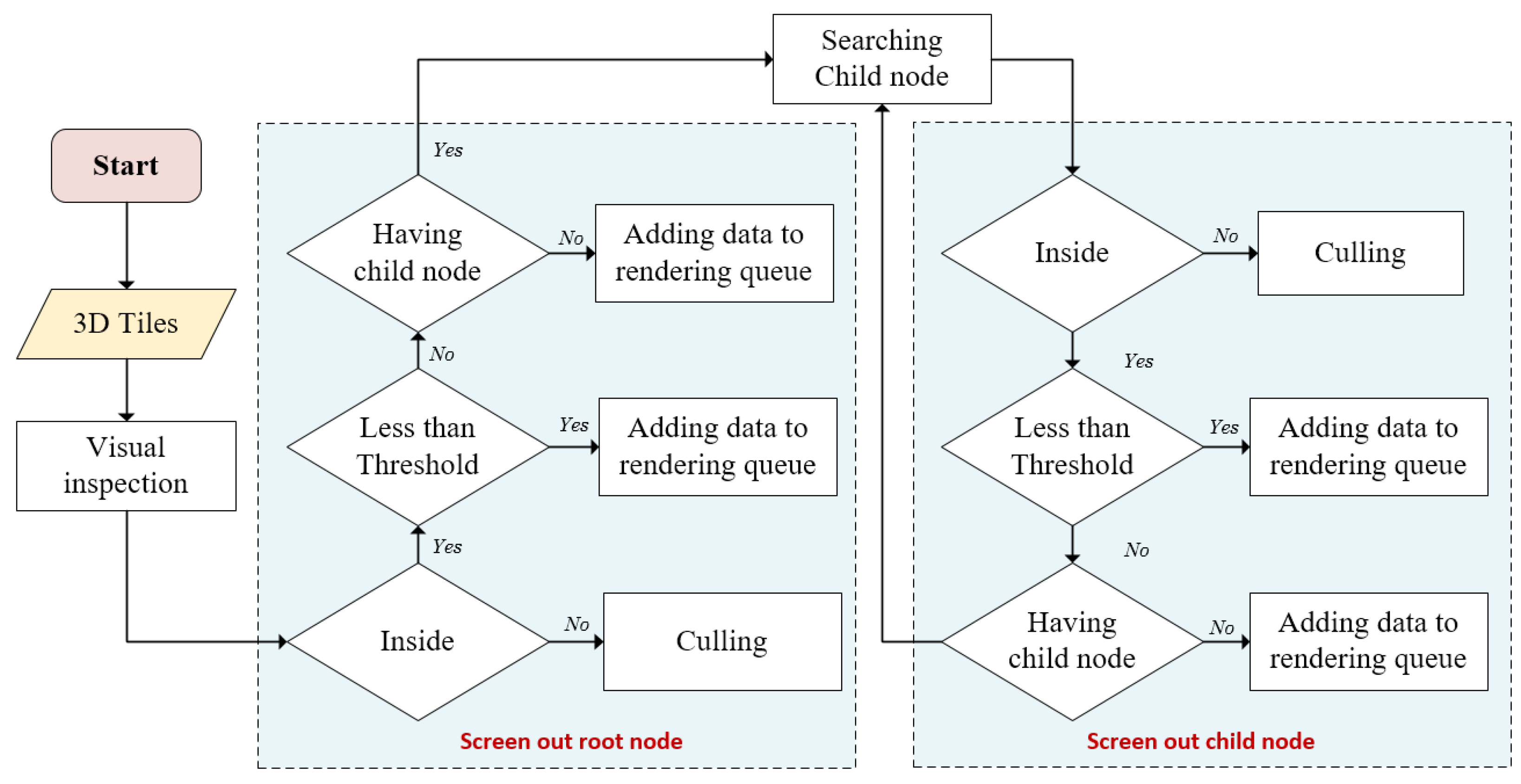
3.1. Scheduling Strategy for 3D Tiles in Cesium
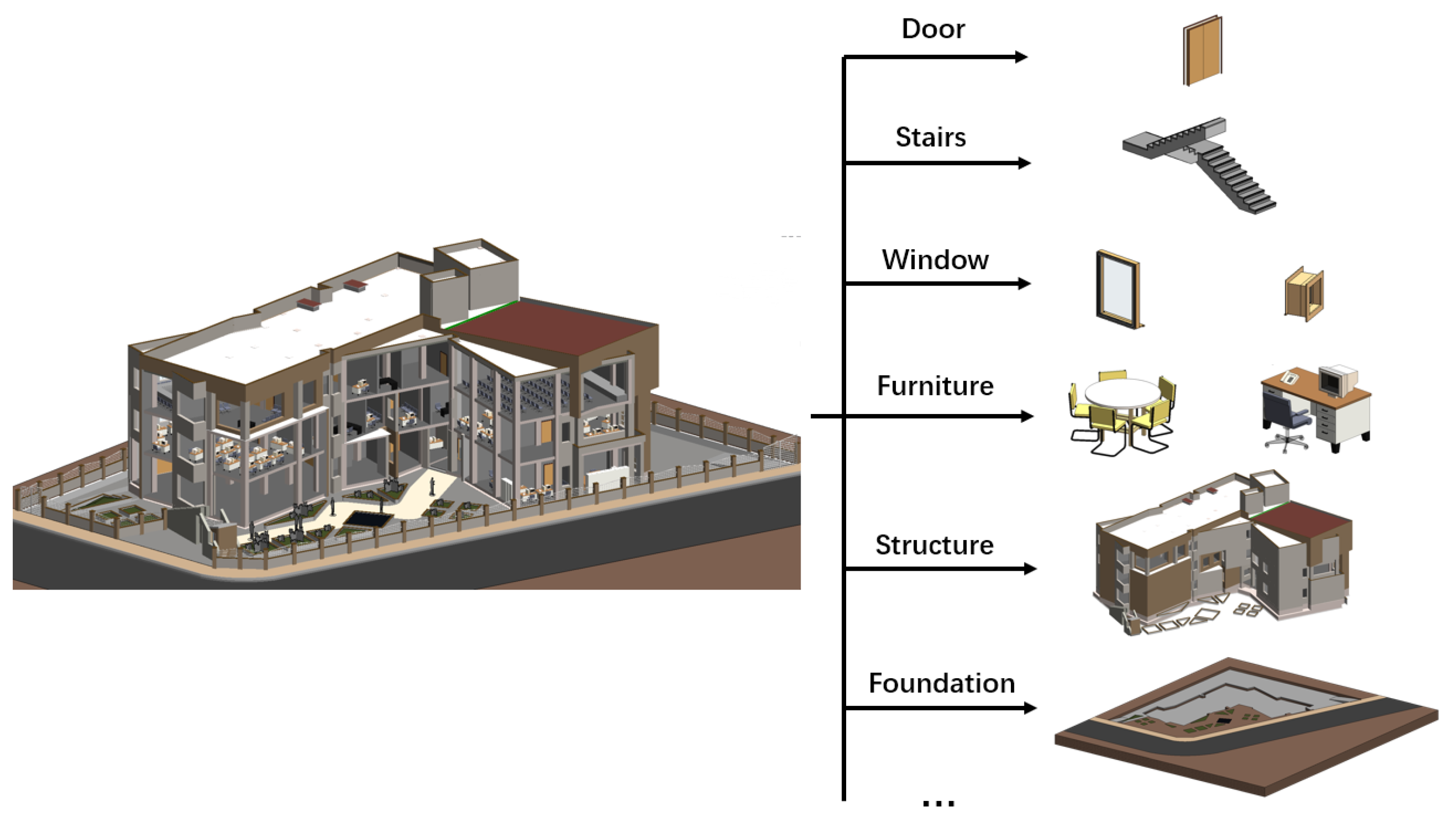
3.2. Data Organization for BIM Models
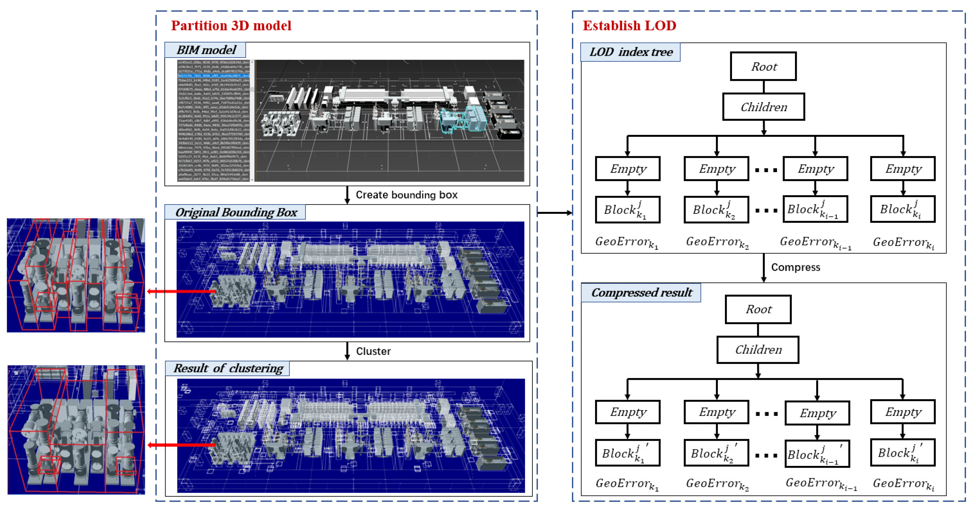
3.2.1. Tiling Method for BIM Models
| Algorithm 1 Tiling method for BIM model |
| Input: |
| Original BIM model |
| Initialize: |
| (1) Analyze the original BIM model and determine the number of subassemblies . |
| (2) Store vertex v, normal vector coordinate vn, texture coordinate vt, and face index f in the corresponding array of subassembly Obj(v, vn, vt, f). |
| (3) Initialize the two-dimensional array of distance and one-dimensional array of minimum bounding cuboids . |
| (4) According to Formula (3), calculate the threshold of clustering . Model Tiling: |
| For each , calculate its minimum bounding cuboid , and the barycenter (calculated using Formula (4)). |
| For each , calculate the distance between itself and other based on and , and add to . |
| While the size of is not zero: |
| Retrieve the minimum distance from and obtain the corresponding subassemblies and . |
| If the sum of and is less than : |
| Update the to the overall minimum bounding cuboid of and , organize all geometrical data in into , and delete and |
| According to Formula (5), recalculate the overall barycenter . |
| Delete in and recalculate the distance between and other . |
| Else: |
| Delete and in . |
| Output: |
| Partitioned BIM model |
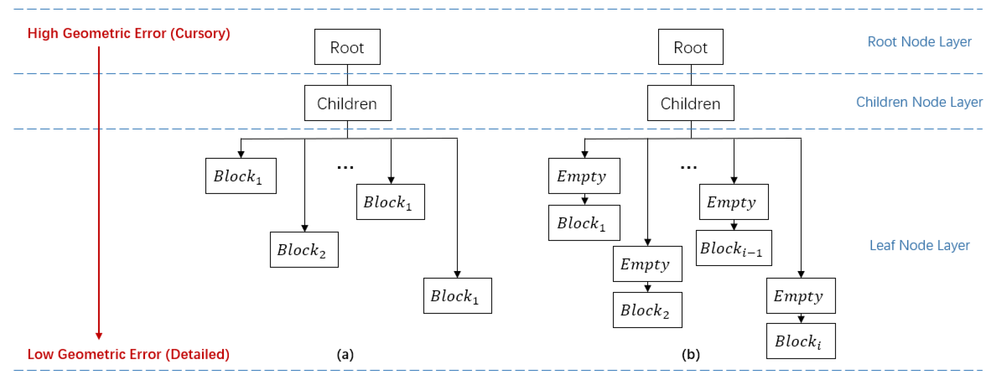
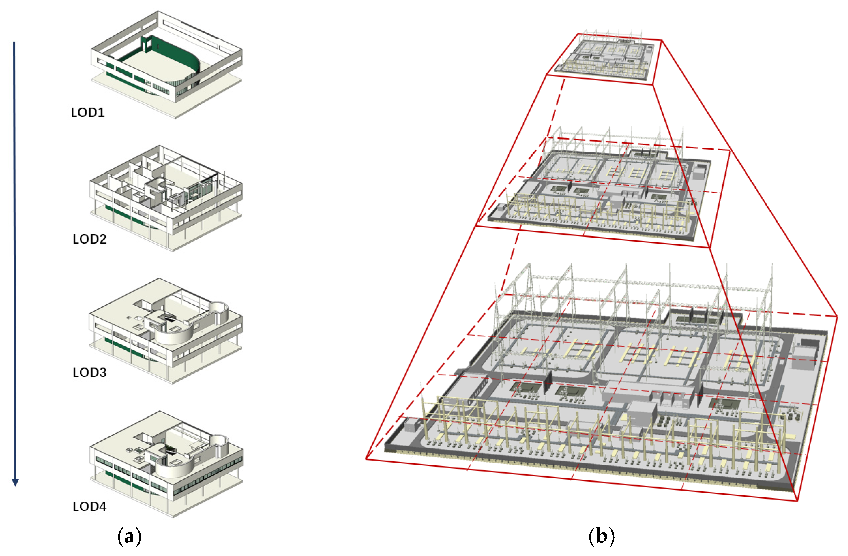
3.2.2. LOD Method for BIM Models
4. Experiments and Discussion
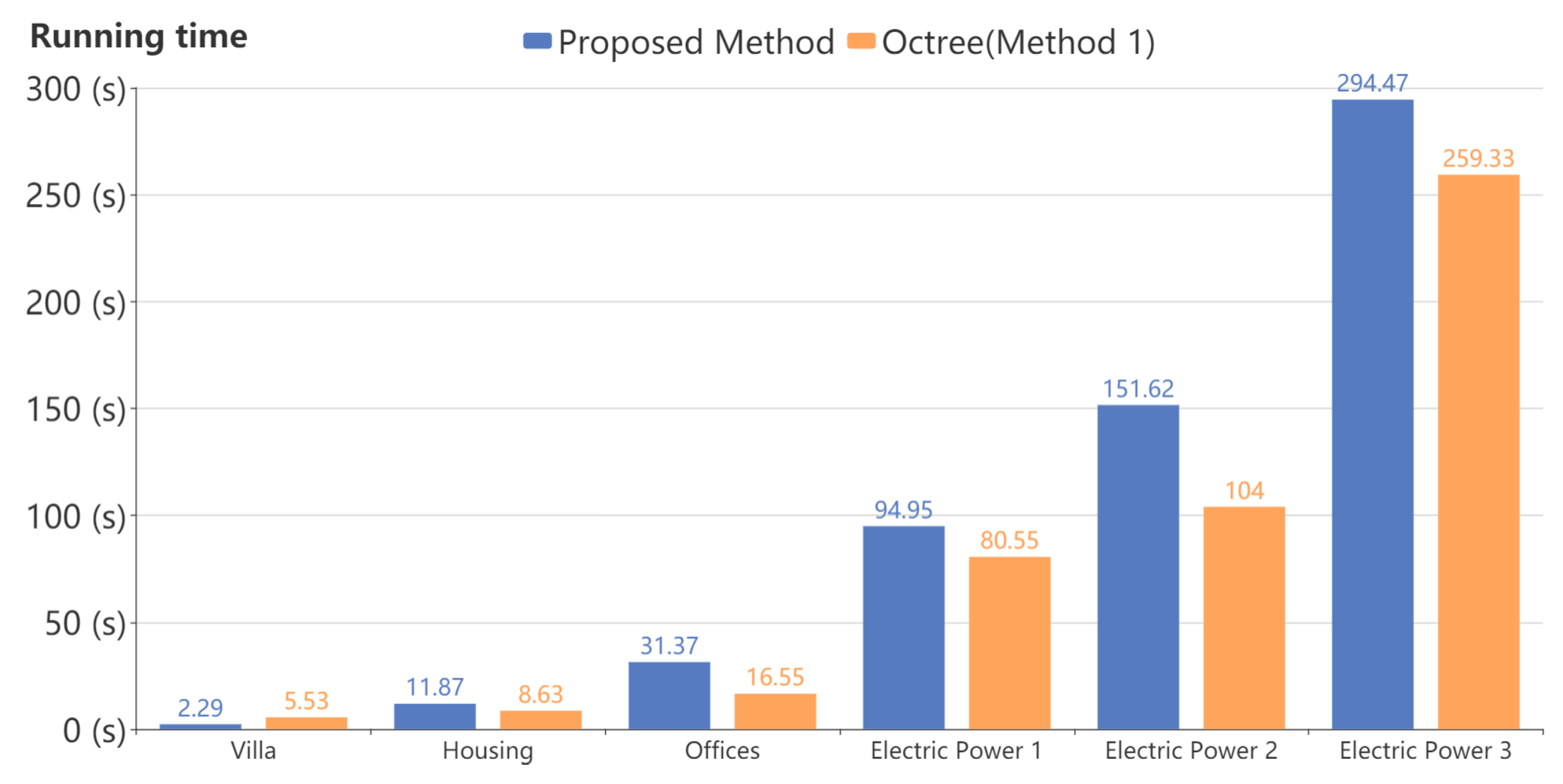
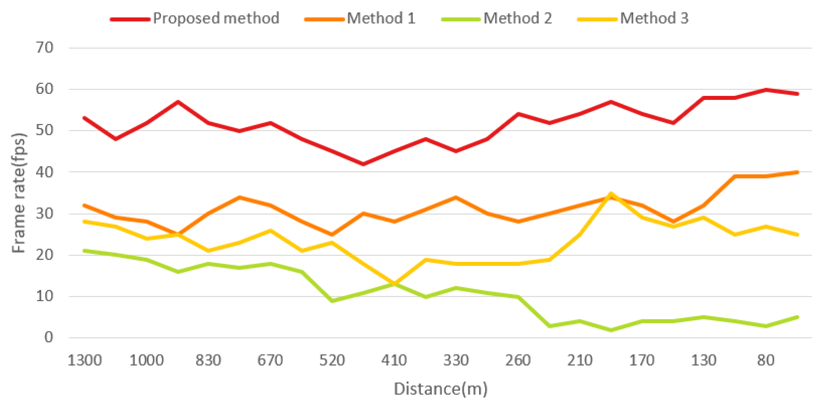
4.1. Performance
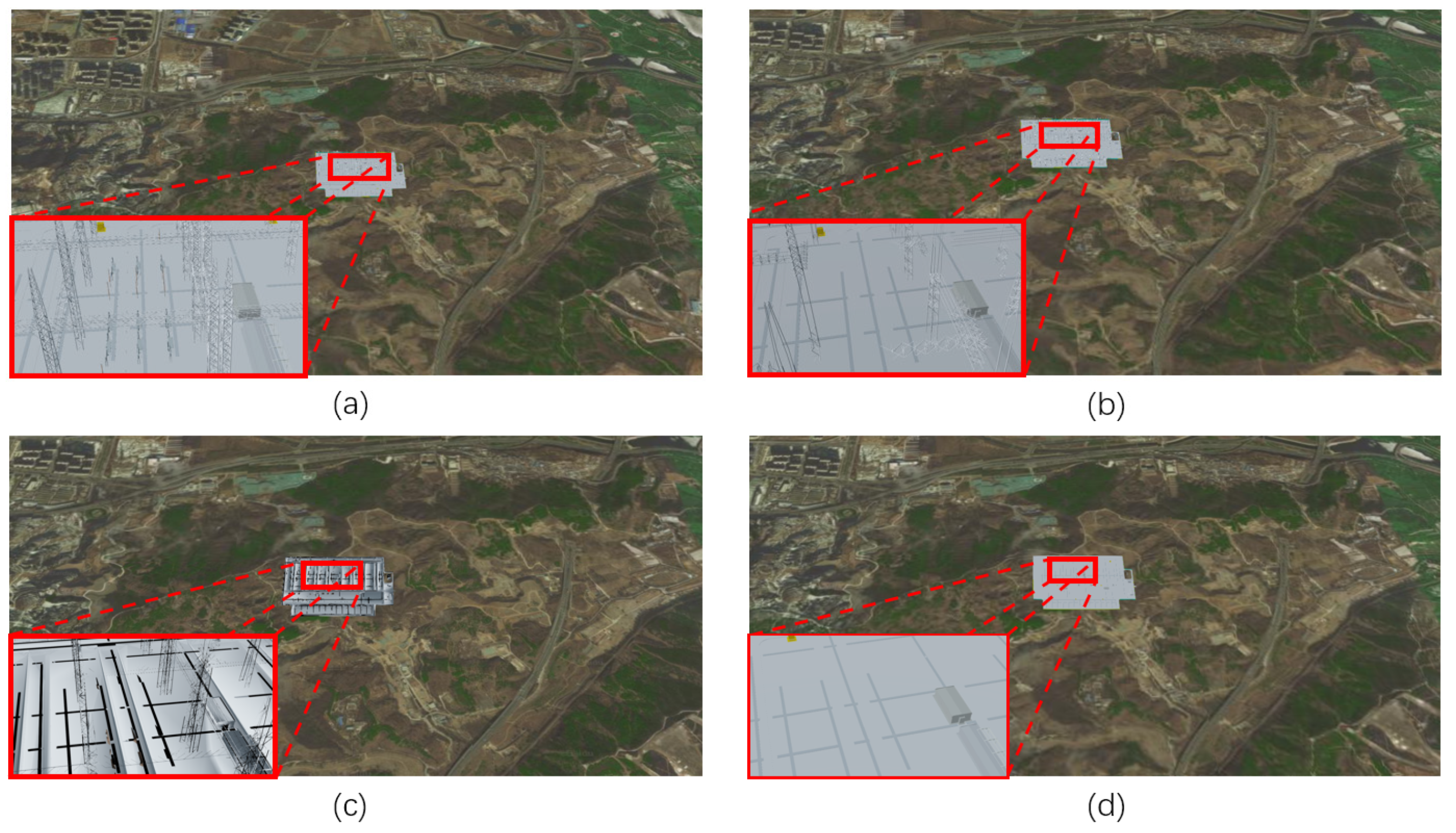
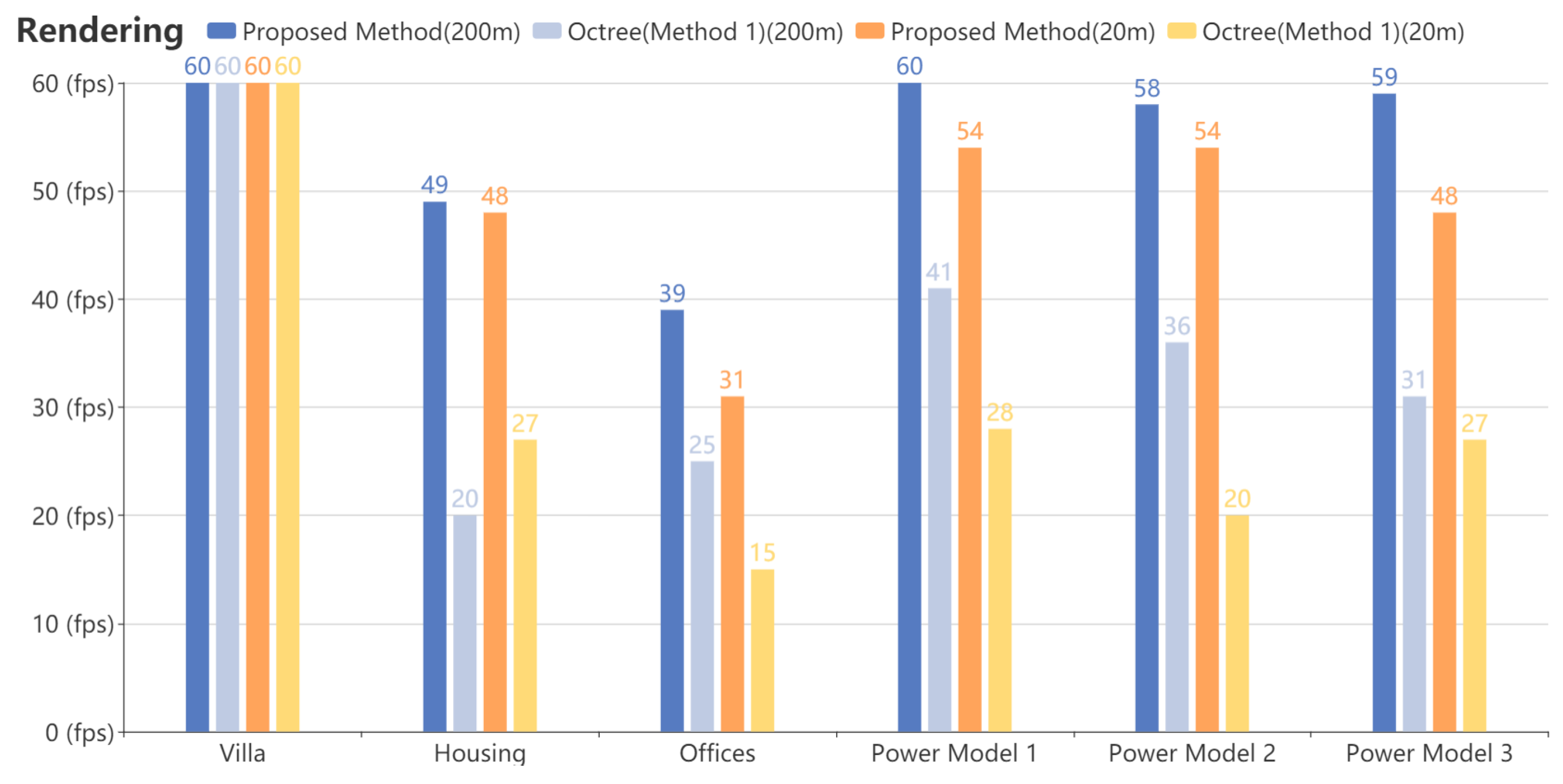
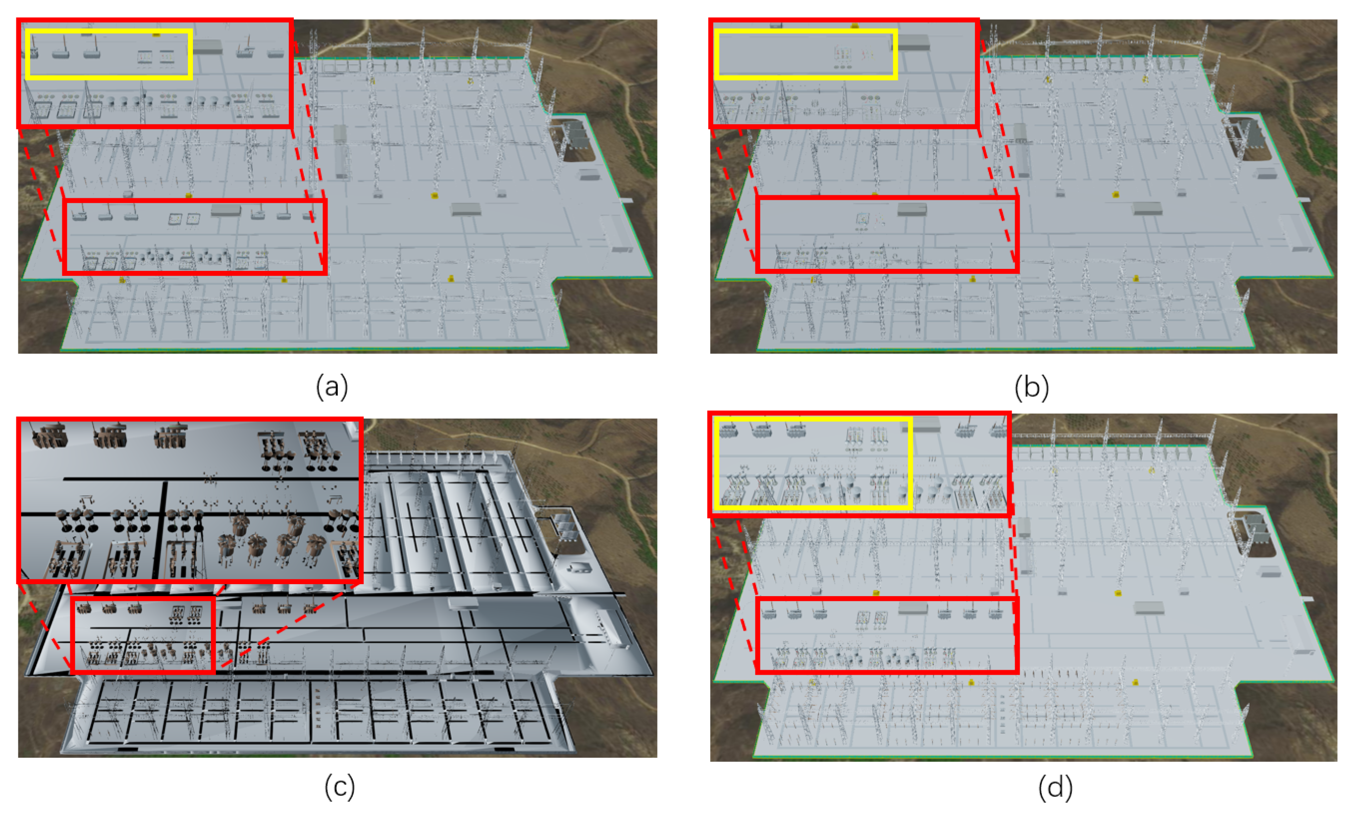
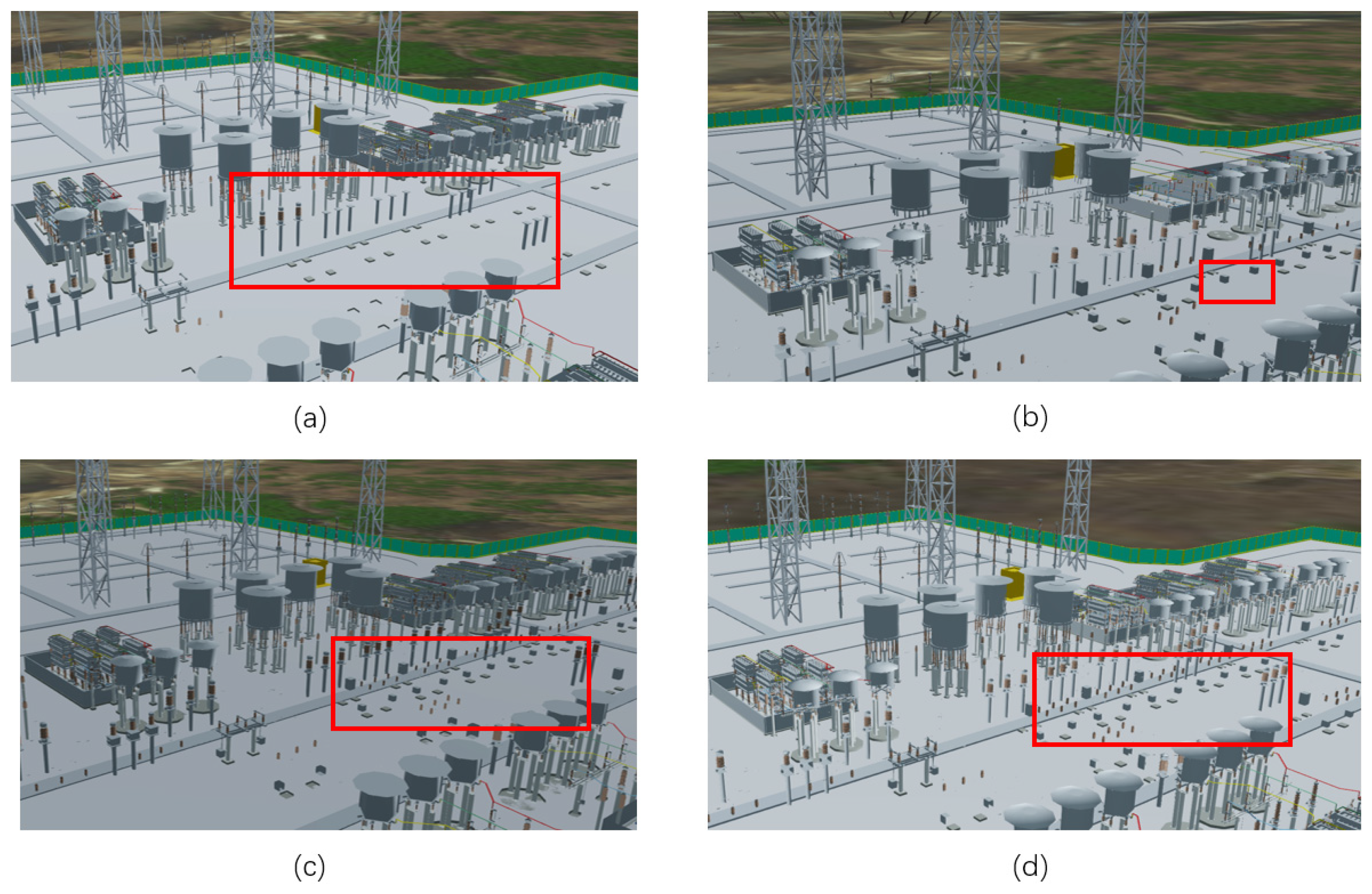
4.2. Comparison of Visualization Afforded by Different Algorithms
5. Conclusions
Author Contributions
Funding
Institutional Review Board Statement
Informed Consent Statement
Data Availability Statement
Acknowledgments
Conflicts of Interest
References
- Howell, S.; Hippolyte, J.-L.; Jayan, B.; Reynolds, J.; Rezgui, Y. Web-Based 3D Urban Decision Support through Intelligent and Interoperable Services. In Proceedings of the 2016 IEEE International Smart Cities Conference (ISC2), Trento, Italy, 12–15 September 2016; pp. 1–4. [Google Scholar]
- Liang, J.; Gong, J.; Li, W. Applications and Impacts of Google Earth: A Decadal Review (2006–2016). ISPRS J. Photogramm. Remote Sens. 2018, 146, 91–107. [Google Scholar] [CrossRef]
- Qiu, G.; Chen, J. Web-Based 3D Map Visualization Using WebGL. In Proceedings of the 2018 13th IEEE Conference on Industrial Electronics and Applications (ICIEA), Wuhan, China, 31 May–2 June 2018; pp. 759–763. [Google Scholar]
- Azhar, S. Building Information Modeling (BIM): Trends, Benefits, Risks, and Challenges for the AEC Industry. Leadersh. Manag. Eng. 2011, 11, 241–252. [Google Scholar] [CrossRef]
- Hooper, M. Automated Model Progression Scheduling Using Level of Development. Constr. Innov. 2015, 15, 428–448. [Google Scholar] [CrossRef]
- 3DTiles. Available online: https://github.com/AnalyticalGraphicsInc/3d-tiles/tree/master/specification#tile-format-specifications/ (accessed on 6 July 2020).
- I3S. Available online: http://docs.opengeospatial.org/cs/17-014r7/17-014r7.html/ (accessed on 7 April 2021).
- S3M. Available online: https://github.com/SuperMap/s3m-spec/tree/master/Specification/ (accessed on 22 June 2021).
- Yang, L.; Zhang, L.; Ma, J.; Xie, J.; Liu, L. Interactive Visualization of Multi-Resolution Urban Building Models Considering Spatial Cognition. Int. J. Geogr. Inf. Sci. 2011, 25, 5–24. [Google Scholar] [CrossRef]
- Chen, Y.; Shooraj, E.; Rajabifard, A.; Sabri, S. From IFC to 3D Tiles: An Integrated Open-Source Solution for Visualising BIMs on Cesium. ISPRS Int. J. Geo. Inf. 2018, 7, 393. [Google Scholar] [CrossRef] [Green Version]
- Mao, B.; Ban, Y.; Laumert, B. Dynamic Online 3D Visualization Framework for Real-Time Energy Simulation Based on 3D Tiles. ISPRS Int. J. Geo. Inf. 2020, 9, 166. [Google Scholar] [CrossRef] [Green Version]
- Song, Z.; Li, J. A Dynamic Tiles Loading and Scheduling Strategy for Massive Oblique Photogrammetry Models. In Proceedings of the 2018 IEEE 3rd International Conference on Image, Vision and Computing (ICIVC), Chongqing, China, 27–29 June 2018; pp. 648–652. [Google Scholar]
- Kulawiak, M.; Kulawiak, M.; Lubniewski, Z. Integration, Processing and Dissemination of LiDAR Data in a 3D Web-GIS. ISPRS Int. J. Geo. Inf. 2019, 8, 144. [Google Scholar] [CrossRef] [Green Version]
- Lu, M.; Wang, X.; Liu, X.; Chen, M.; Bi, S.; Zhang, Y.; Lao, T. Web-Based Real-Time Visualization of Large-Scale Weather Radar Data Using 3D Tiles. Trans. GIS 2021, 25, 25–43. [Google Scholar] [CrossRef]
- Herman, L.; Russnák, J.; Řezník, T. Flood Modelling and Visualizations of Floods Through 3D Open Data. In International Symposium on Environmental Software Systems; Hřebíček, J., Denzer, R., Schimak, G., Pitner, T., Eds.; Springer International Publishing: Cham, Switzerland, 2017; pp. 139–149. [Google Scholar]
- Xu, Z.; Zhang, L.; Li, H.; Lin, Y.-H.; Yin, S. Combining IFC and 3D Tiles to Create 3D Visualization for Building Information Modeling. Autom. Constr. 2020, 109, 102995. [Google Scholar] [CrossRef]
- Kim, J.; Hong, C.; Son, S. A Light Weight Algorithm for Large-Scale BIM Data for Visualization on a Web-Based GIS Platform. Build. Inf. Model. (BIM) Des. Constr. Oper. 2015, 149, 355–367. [Google Scholar]
- Hu, Z.-Z.; Yuan, S.; Benghi, C.; Zhang, J.-P.; Zhang, X.-Y.; Li, D.; Kassem, M. Geometric Optimization of Building Information Models in MEP Projects: Algorithms and Techniques for Improving Storage, Transmission and Display. Autom. Constr. 2019, 107, 102941. [Google Scholar] [CrossRef]
- Chen, J.; Li, J.; Li, M. Progressive Visualization of Complex 3D Models Over the Internet. Trans. GIS 2016, 20, 887–902. [Google Scholar] [CrossRef]
- Chen, J.; Li, M.; Li, J. An Improved Texture-Related Vertex Clustering Algorithm for Model Simplification. Comput. Geosci. 2015, 83, 37–45. [Google Scholar] [CrossRef]
- Ziolkowska, J.R.; Reyes, R. Geological and Hydrological Visualization Models for Digital Earth Representation. Comput. Geosci. 2016, 94, 31–39. [Google Scholar] [CrossRef] [Green Version]
- Kulawiak, M.; Kulawiak, M. Application of Web-GIS for Dissemination and 3D Visualization of Large-Volume LiDAR Data. In The Rise of Big Spatial Data; Ivan, I., Singleton, A., Horák, J., Inspektor, T., Eds.; Springer International Publishing: Cham, Switzerland, 2017; pp. 1–12. [Google Scholar]
- Cozzi, P.J. Visibility Driven Out-of-Core Hlod Rendering. Master’s Thesis, University of Pennsylvania, Philadelphia, PA, USA, 2008. [Google Scholar]
- Draco. Available online: https://github.com/google/draco.html/ (accessed on 21 July 2020).
- Hoppe, H. View-Dependent Refinement of Progressive Meshes. ACM SIGGRAPH 1997, 189–198. [Google Scholar] [CrossRef] [Green Version]
- Cesium3DTileset. Available online: https://cesium.com/docs/cesiumjs-ref-doc/Cesium3DTileset.html/ (accessed on 6 July 2020).


| Model Name | Model Size(.obj) | Number of Faces | Thumbnail Image |
|---|---|---|---|
| Villa | 3.25 MB | 47,370 |  |
| Housing | 25.3 MB | 203,187 |  |
| Offices | 91.0 MB | 540,964 |  |
| Electric Power 1 | 694 MB | 5,882,088 |  |
| Electric Power 2 | 1.0 GB | 7,403,652 |  |
| Electric Power 3 | 2.84 GB | 11,021,840 |  |
| Proposed Method | Octree(Method 1) | |
|---|---|---|
| Villa |  | 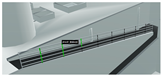 |
| Housing | 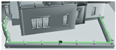 | 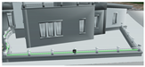 |
| Offices | 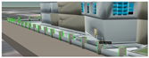 | 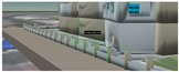 |
| Electric Power 1 | 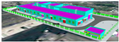 |  |
| Electric Power 2 | 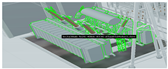 | 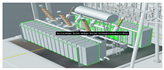 |
| Electric Power 3 | 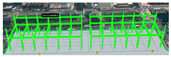 | 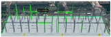 |
Publisher’s Note: MDPI stays neutral with regard to jurisdictional claims in published maps and institutional affiliations. |
© 2021 by the authors. Licensee MDPI, Basel, Switzerland. This article is an open access article distributed under the terms and conditions of the Creative Commons Attribution (CC BY) license (https://creativecommons.org/licenses/by/4.0/).
Share and Cite
Zhan, W.; Chen, Y.; Chen, J. 3D Tiles-Based High-Efficiency Visualization Method for Complex BIM Models on the Web. ISPRS Int. J. Geo-Inf. 2021, 10, 476. https://doi.org/10.3390/ijgi10070476
Zhan W, Chen Y, Chen J. 3D Tiles-Based High-Efficiency Visualization Method for Complex BIM Models on the Web. ISPRS International Journal of Geo-Information. 2021; 10(7):476. https://doi.org/10.3390/ijgi10070476
Chicago/Turabian StyleZhan, Wenxiao, Yuxuan Chen, and Jing Chen. 2021. "3D Tiles-Based High-Efficiency Visualization Method for Complex BIM Models on the Web" ISPRS International Journal of Geo-Information 10, no. 7: 476. https://doi.org/10.3390/ijgi10070476
APA StyleZhan, W., Chen, Y., & Chen, J. (2021). 3D Tiles-Based High-Efficiency Visualization Method for Complex BIM Models on the Web. ISPRS International Journal of Geo-Information, 10(7), 476. https://doi.org/10.3390/ijgi10070476