
Temporal and Spatial Evolution Analysis of Earthquake Events in California and Nevada Based on Spatial Statistics


Abstract
:1. Introduction
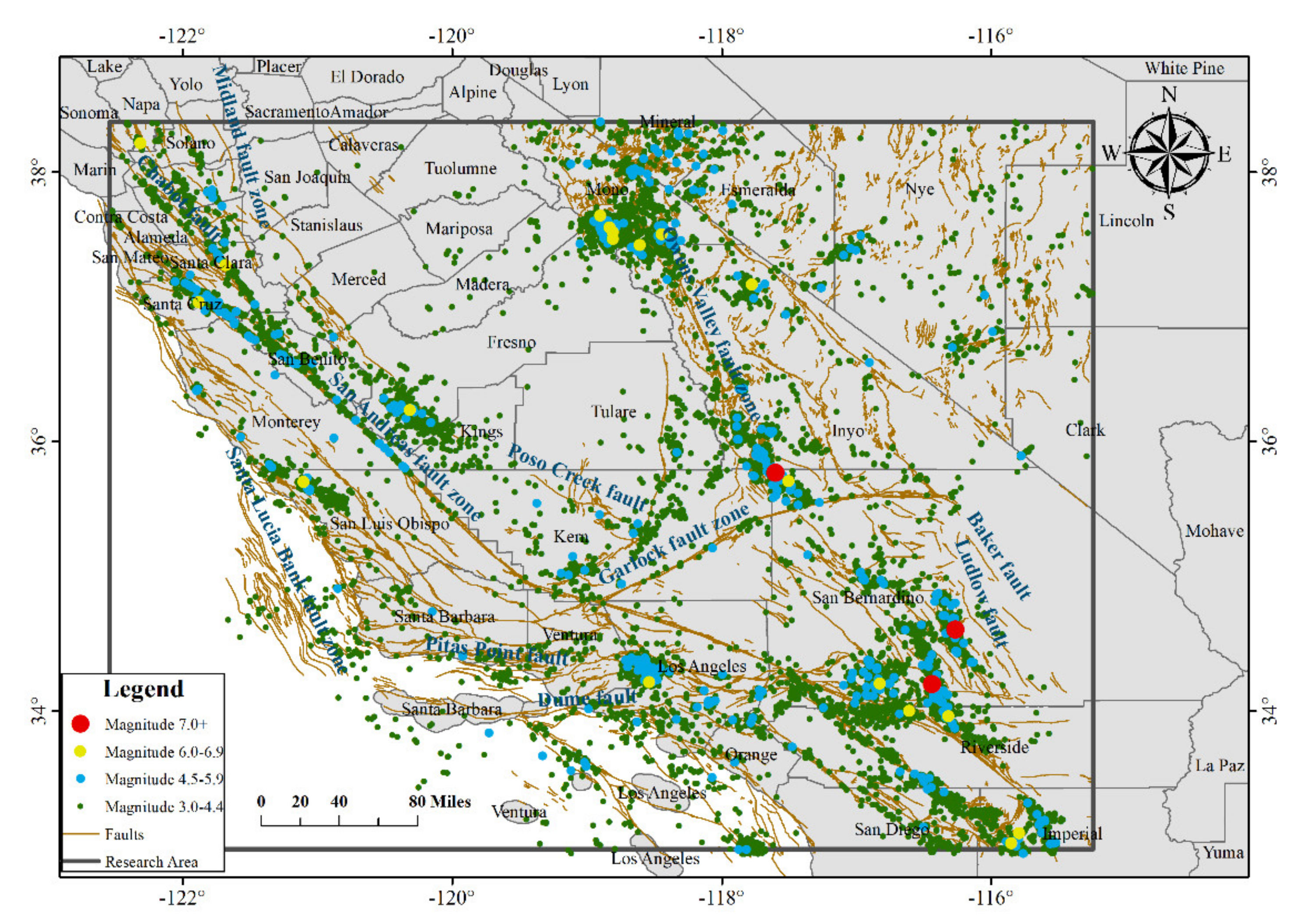
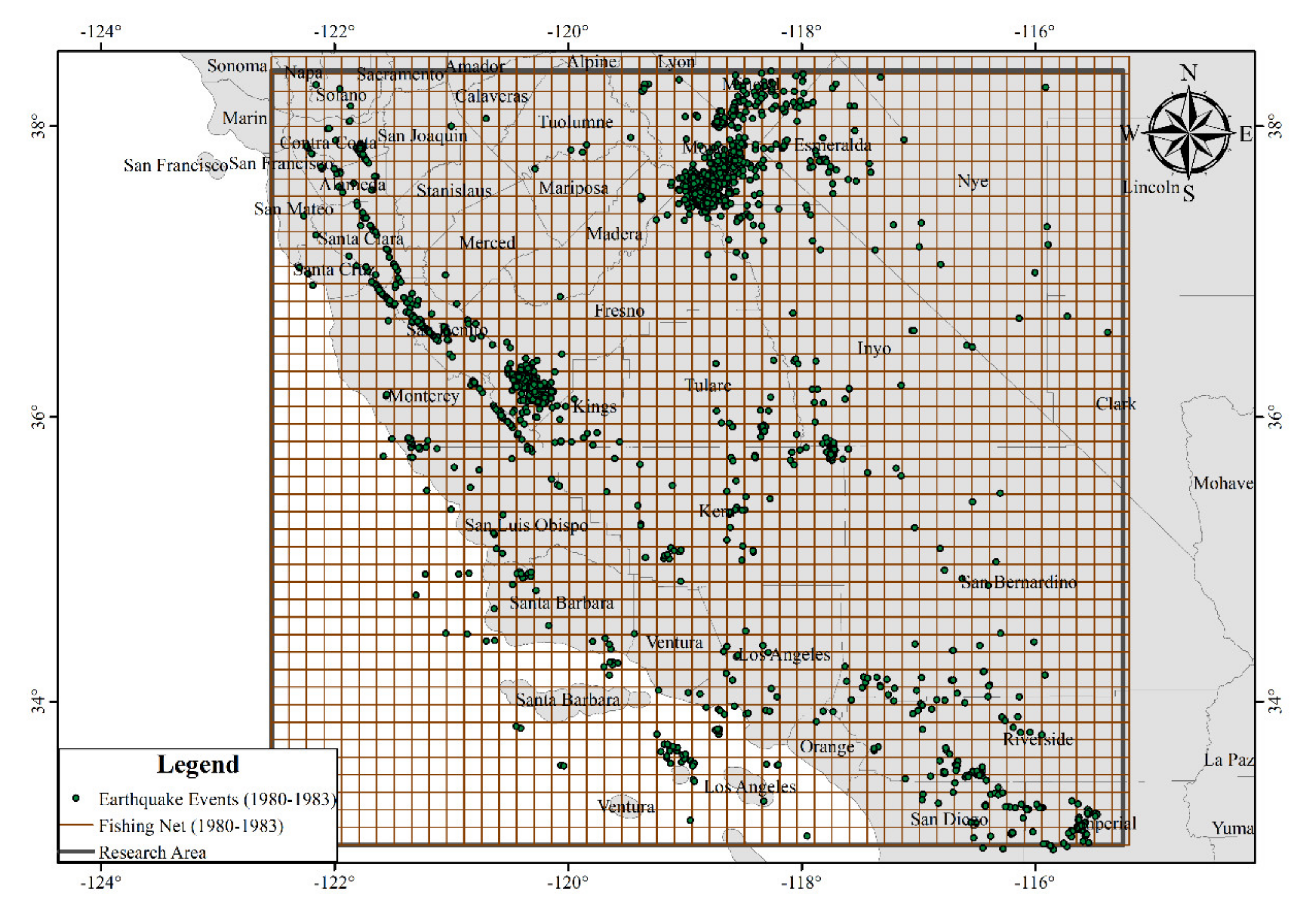
2. Study Area
3. Method
3.1. Weighted Average Center
3.2. Standard Deviational Ellipse
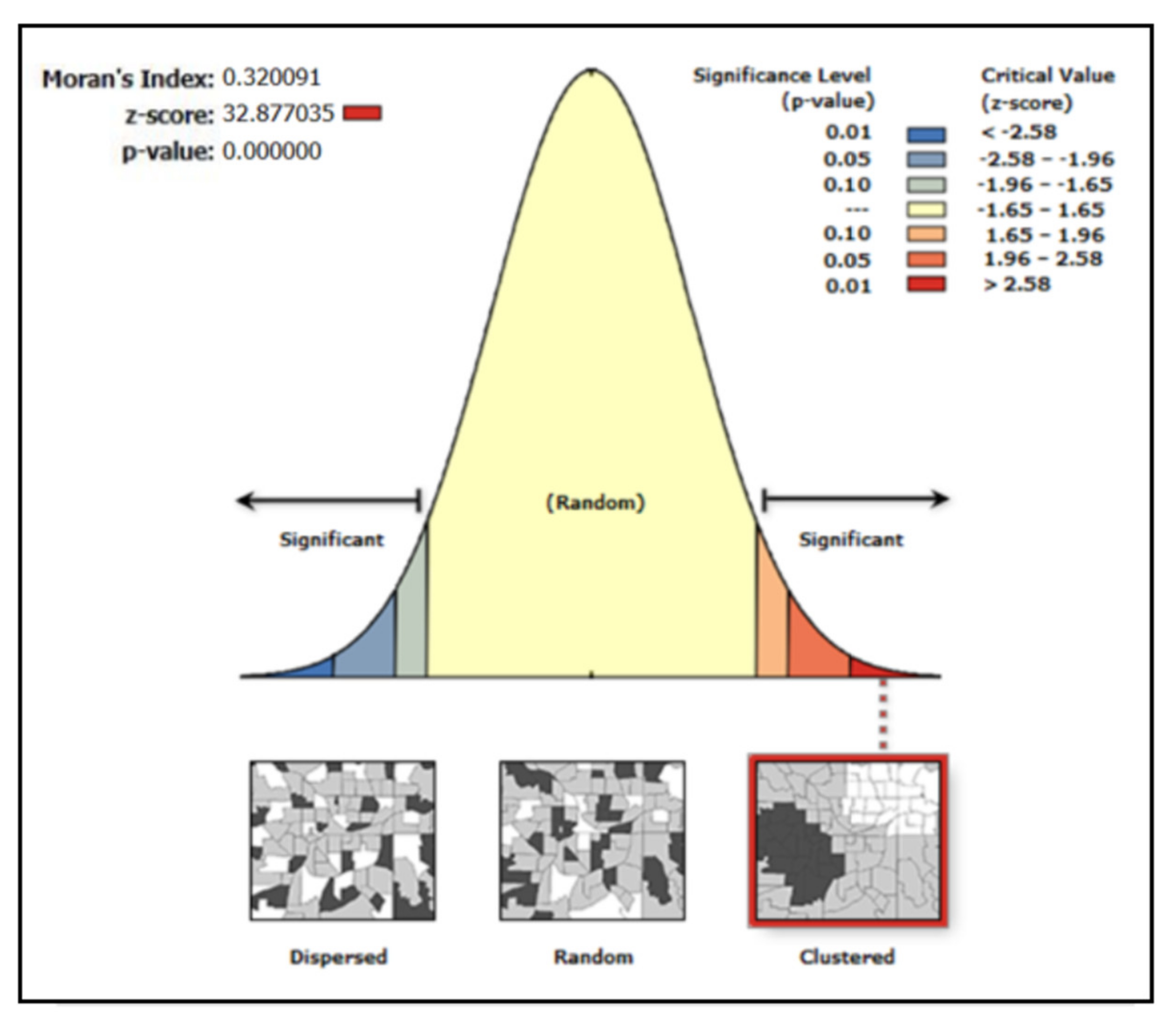
3.3. Global Spatial Autocorrelation Analysis
4. Results
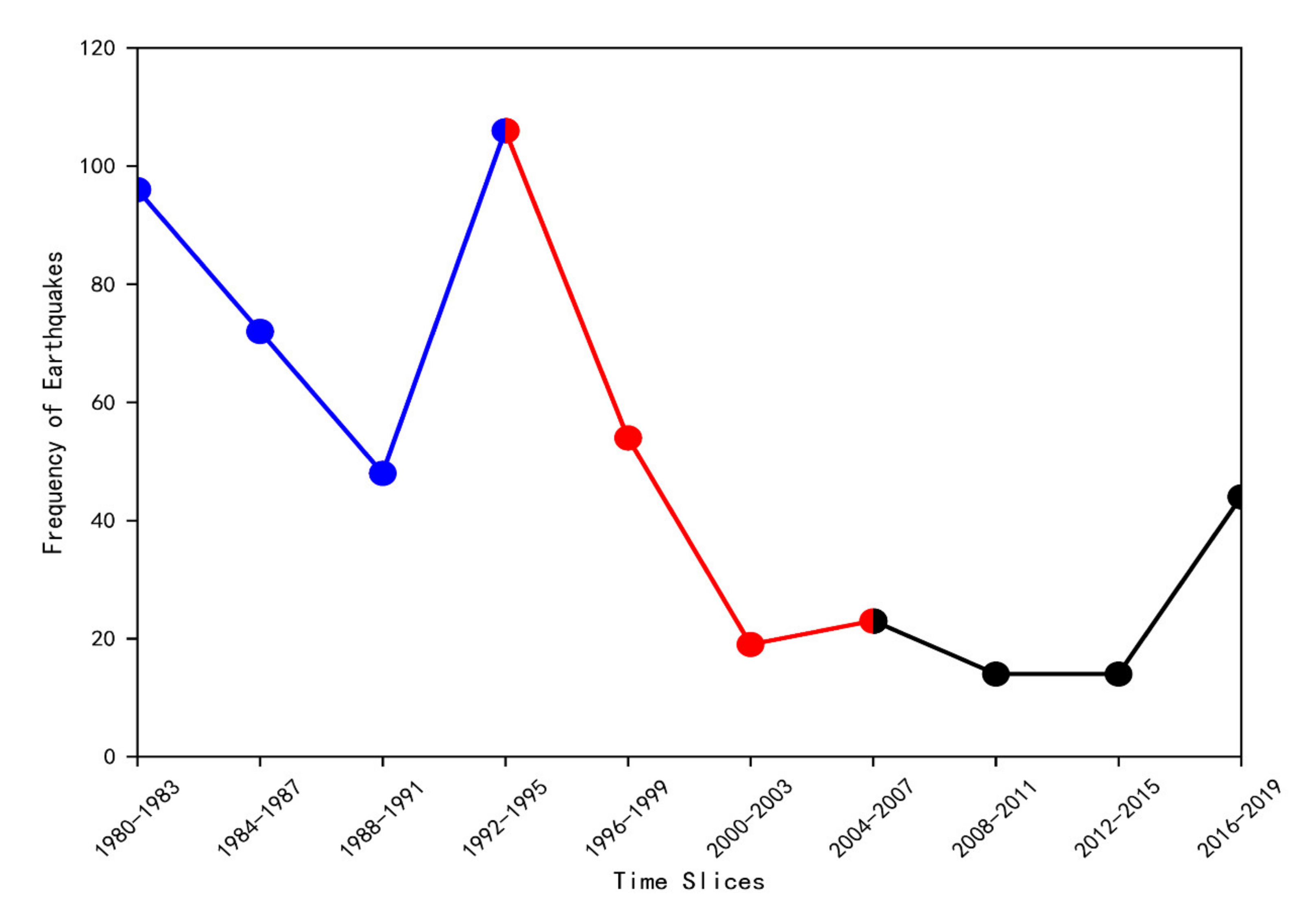
4.1. Frequency Statistical Results
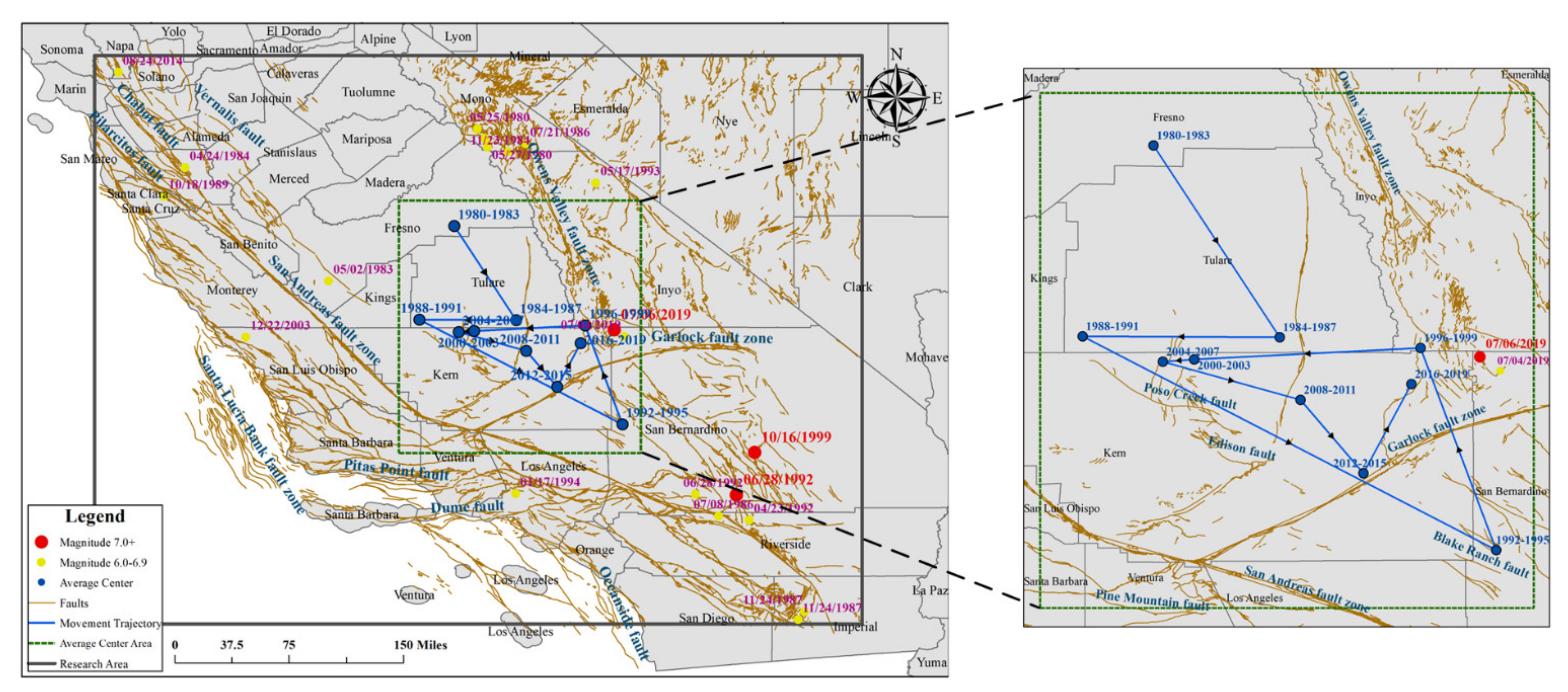
4.2. Temporal and Spatial Evolution Process of the Weighted Average Center of Earthquake Events
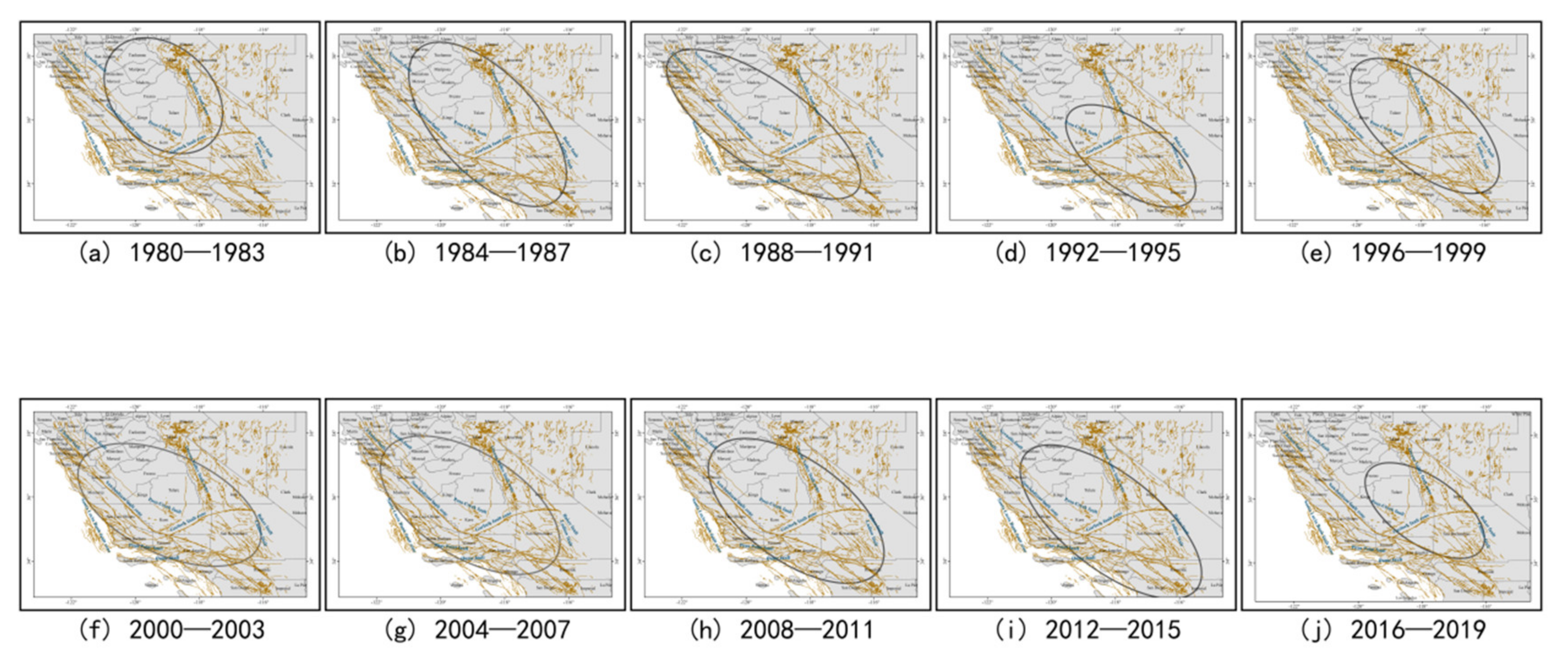
4.3. Temporal and Spatial Evolution Process of the SDE
4.4. Temporal and Spatial Evolution Process of Global Spatial Autocorrelation Analysis
5. Discussion and Conclusions
Author Contributions
Funding
Acknowledgments
Conflicts of Interest
References
- Nelson, A.C.; French, S.P. Plan quality and mitigating damage from natural disasters: A case study of the Northridge earthquake with planning policy considerations. J. Am. Plan. Assoc. 2002, 68, 194–207. [Google Scholar] [CrossRef]
- Vina, A.; Chen, X.; McConnell, W.J.; Liu, W.; Xu, W.; Ouyang, Z.; Zhang, H.; Liu, J. Effects of natural disasters on conservation policies: The case of the 2008 Wenchuan Earthquake, China. Ambio 2011, 40, 274–284. [Google Scholar] [CrossRef] [PubMed] [Green Version]
- Scawthorn, C.; O’rourke, T.; Blackburn, F. The 1906 San Francisco earthquake and fire—Enduring lessons for fire protection and water supply. Earthq. Spectra 2006, 22, 135–158. [Google Scholar] [CrossRef]
- Odell, K.A.; Weidenmier, M.D. Real shock, monetary aftershock: The 1906 San Francisco earthquake and the panic of 1907. J. Econ. Hist. 2004, 64, 1002–1027. [Google Scholar] [CrossRef] [Green Version]
- Geller, R.J. Earthquake prediction: A critical review. Geophys. J. Int. 1997, 131, 425–450. [Google Scholar] [CrossRef] [Green Version]
- Chan, C.-H.; Wu, Y.-M.; Tseng, T.-L.; Lin, T.-L.; Chen, C.-C. Spatial and temporal evolution of b-values before large earthquakes in Taiwan. Tectonophysics 2012, 532, 215–222. [Google Scholar] [CrossRef] [Green Version]
- Song, Z.-p.; Yin, X.-c.; Wang, Y.-c.; Xu, P.; Xue, Y. The tempo-spatial evolution characteristics of the load/unload response ratio before strong earthquakes in California of America and its predicting implications. Acta Seismol. Sin. 2000, 13, 628–635. [Google Scholar] [CrossRef]
- Unwin, D.J. GIS, spatial analysis and spatial statistics. Prog. Hum. Geogr. 1996, 20, 540–551. [Google Scholar] [CrossRef]
- Wagner, H.H.; Fortin, M.-J. Spatial analysis of landscapes: Concepts and statistics. Ecology 2005, 86, 1975–1987. [Google Scholar] [CrossRef] [Green Version]
- Páez, A.; Scott, D.M. Spatial statistics for urban analysis: A review of techniques with examples. GeoJournal 2004, 61, 53–67. [Google Scholar] [CrossRef]
- Rosenberg, M.S.; Anderson, C.D. PASSaGE: Pattern analysis, spatial statistics and geographic exegesis. Version 2. Methods Ecol. Evol. 2011, 2, 229–232. [Google Scholar] [CrossRef]
- Gan, B.-r.; Yang, X.-g.; Zhang, W.; Zhou, J.-w. Temporal and Spatial Evolution of Vegetation Coverage in the Mianyuan River Basin Influenced by Strong Earthquake Disturbance. Sci. Rep. 2019, 9, 16762. [Google Scholar] [CrossRef]
- Wang, X.; Zhuo, L.; Li, C.; Engel, B.A.; Sun, S.; Wang, Y. Temporal and spatial evolution trends of drought in northern Shaanxi of China: 1960–2100. Theor. Appl. Climatol. 2020, 139, 965–979. [Google Scholar] [CrossRef]
- He, Z.; Zhao, C.; Zhou, Q.; Liang, H. Temporal--spatial evolution of the lagged effect of Karst drainage basin for rainfall-runoff in Central Guizhou of China. Authorea Prepr. 2020. [Google Scholar] [CrossRef]
- Zhang, S.; Li, R.; Wang, F.; Iio, A. Characteristics of landslides triggered by the 2018 Hokkaido Eastern Iburi earthquake, Northern Japan. Landslides 2019, 16, 1691–1708. [Google Scholar] [CrossRef]
- Qi, S.; Xu, Q.; Lan, H.; Zhang, B.; Liu, J. Spatial distribution analysis of landslides triggered by 2008. 5. 12 Wenchuan Earthquake, China. Eng. Geol. 2010, 116, 95–108. [Google Scholar] [CrossRef]
- Dias, V.H.; Papa, A.R.; Ferreira, D.S. Analysis of temporal and spatial distributions between earthquakes in the region of California through Non-Extensive Statistical Mechanics and its limits of validity. Phys. A Stat. Mech. Its Appl. 2019, 529, 121471. [Google Scholar] [CrossRef]
- Yang, J.; Cheng, C.; Song, C.; Shen, S.; Zhang, T.; Ning, L. Spatial-temporal distribution characteristics of global seismic clusters and associated spatial factors. Chin. Geogr. Sci. 2019, 29, 614–625. [Google Scholar] [CrossRef] [Green Version]
- Huang, H.; Meng, L.; Bürgmann, R.; Wang, W.; Wang, K. Spatio-temporal foreshock evolution of the 2019 M 6. 4 and M 7.1 Ridgecrest, California earthquakes. Earth Planet. Sci. Lett. 2020, 551, 116582. [Google Scholar] [CrossRef]
- Jena, R.; Pradhan, B. Integrated ANN-cross-validation and AHP-TOPSIS model to improve earthquake risk assessment. Int. J. Disaster Risk Reduct. 2020, 50, 101723. [Google Scholar] [CrossRef]
- Jia, Y.; Ma, J. What can machine learning do for seismic data processing? An interpolation application. Geophysics 2017, 82, V163–V177. [Google Scholar] [CrossRef]
- DeVries, P.M.; Viégas, F.; Wattenberg, M.; Meade, B.J. Deep learning of aftershock patterns following large earthquakes. Nature 2018, 560, 632–634. [Google Scholar] [CrossRef] [PubMed]
- Karimzadeh, S.; Matsuoka, M.; Kuang, J.; Ge, L. Spatial prediction of aftershocks triggered by a major earthquake: A binary machine learning perspective. ISPRS Int. J. Geo-Inf. 2019, 8, 462. [Google Scholar] [CrossRef] [Green Version]
- Mignan, A.; Broccardo, M. One neuron versus deep learning in aftershock prediction. Nature 2019, 574, E1–E3. [Google Scholar] [CrossRef]
- Toppozada, T.R.; Branum, D.; Reichle, M.; Hallstrom, C. San Andreas fault zone, California: M ≥ 5.5 earthquake history. Bull. Seismol. Soc. Am. 2002, 92, 2555–2601. [Google Scholar] [CrossRef]
- Wu, D.; Mendel, J.M. Aggregation using the linguistic weighted average and interval type-2 fuzzy sets. IEEE Trans. Fuzzy Syst. 2007, 15, 1145–1161. [Google Scholar] [CrossRef]
- Kent, J.; Leitner, M. Efficacy of standard deviational ellipses in the application of criminal geographic profiling. J. Investig. Psychol. Offender Profiling 2007, 4, 147–165. [Google Scholar] [CrossRef]
- Eryando, T.; Susanna, D.; Pratiwi, D.; Nugraha, F. Standard Deviational Ellipse (SDE) models for malaria surveillance, case study: Sukabumi district-Indonesia, in 2012. Malar. J. 2012, 11, P130. [Google Scholar] [CrossRef] [Green Version]
- Wang, B.; Shi, W.; Miao, Z. Confidence analysis of standard deviational ellipse and its extension into higher dimensional Euclidean space. PLoS ONE 2015, 10, e0118537. [Google Scholar] [CrossRef]
- Gong, J. Clarifying the standard deviational ellipse. Geogr. Anal. 2002, 34, 155–167. [Google Scholar] [CrossRef]
- Moore, T.W.; McGuire, M.P. Using the standard deviational ellipse to document changes to the spatial dispersion of seasonal tornado activity in the United States. NPJ Clim. Atmos. Sci. 2019, 2, 21. [Google Scholar] [CrossRef]
- Huo, X.-N.; Zhang, W.-W.; Sun, D.-F.; Li, H.; Zhou, L.-D.; Li, B.-G. Spatial pattern analysis of heavy metals in Beijing agricultural soils based on spatial autocorrelation statistics. Int. J. Environ. Res. Public Health 2011, 8, 2074–2089. [Google Scholar] [CrossRef] [Green Version]
- Myint, S.W. Spatial autocorrelation. In Encyclopedia of Geography; Thousand OAKS: London, UK, 2010; pp. 2607–2608. Available online: https://core.ac.uk/download/pdf/6654314.pdf (accessed on 7 December 2019).
- Tsai, P.-J.; Lin, M.-L.; Chu, C.-M.; Perng, C.-H. Spatial autocorrelation analysis of health care hotspots in Taiwan in 2006. BMC Public Health 2009, 9, 464. [Google Scholar] [CrossRef] [Green Version]
- Sui, D.Z. Tobler’s first law of geography: A big idea for a small world? Ann. Assoc. Am. Geogr. 2004, 94, 269–277. [Google Scholar] [CrossRef]
- Miller, H.J. Tobler’s first law and spatial analysis. Ann. Assoc. Am. Geogr. 2004, 94, 284–289. [Google Scholar] [CrossRef]
- Klippel, A.; Hardisty, F.; Li, R. Interpreting spatial patterns: An inquiry into formal and cognitive aspects of Tobler’s first law of geography. Ann. Assoc. Am. Geogr. 2011, 101, 1011–1031. [Google Scholar] [CrossRef]
- Noe, J.P.; Campbell, C.L. Spatial pattern analysis of plant-parasitic nematodes. J. Nematol. 1985, 17, 86. Available online: https://www.ncbi.nlm.nih.gov/pmc/articles/PMC2618431/pdf/86.pdf (accessed on 7 December 2019).
- Usher, M. Analysis of pattern in real and artificial plant populations. J. Ecol. 1975, 569–586. [Google Scholar] [CrossRef]
- Simpson, D. Weighted Averages. Department of Physical Sciences and Engineering, Prince George’s Community. 2010. Available online: http://www.pgccphy.net/ref/weightave.pdf (accessed on 7 December 2019).
- Chen, Y. New approaches for calculating Moran’s index of spatial autocorrelation. PLoS ONE 2013, 8, e68336. [Google Scholar] [CrossRef] [Green Version]
- Al-Ahmadi, K.; Al-Zahrani, A. Spatial autocorrelation of cancer incidence in Saudi Arabia. Int. J. Environ. Res. Public Health 2013, 10, 7207–7228. [Google Scholar] [CrossRef]
- Duncan, D.T.; Kawachi, I.; White, K.; Williams, D.R. The geography of recreational open space: Influence of neighborhood racial composition and neighborhood poverty. J. Urban Health 2013, 90, 618–631. [Google Scholar] [CrossRef] [Green Version]


| No. | Time Slices | Number of Earthquakes | Magnitude 3.0–4.4 | Magnitude 4.5–5.9 | Magnitude 6.0–6.9 | Magnitude 7.0+ |
|---|---|---|---|---|---|---|
| 1 | 1980–1983 | 2840 | 2744 | 91 | 5 | 0 |
| 2 | 1984–1987 | 1988 | 1916 | 66 | 6 | 0 |
| 3 | 1988–1991 | 1294 | 1246 | 47 | 1 | 0 |
| 4 | 1992–1995 | 2934 | 2828 | 101 | 4 | 1 |
| 5 | 1996–1999 | 1860 | 1806 | 53 | 0 | 1 |
| 6 | 2000–2003 | 1034 | 1015 | 18 | 1 | 0 |
| 7 | 2004–2007 | 837 | 814 | 23 | 0 | 0 |
| 8 | 2008–2011 | 727 | 713 | 14 | 0 | 0 |
| 9 | 2012–2015 | 615 | 601 | 13 | 1 | 0 |
| 10 | 2016–2019 | 1633 | 1589 | 42 | 1 | 1 |
| Num. | Time Slice | Area (km2) | XSD (km) | YSD (km) | Rotation (°) |
|---|---|---|---|---|---|
| 1 | 1980–1983 | 154,520.46 | 153.05 | 232.25 | 132.90 |
| 2 | 1984–1987 | 240,296.75 | 157.30 | 355.43 | 136.98 |
| 3 | 1988–1991 | 230,772.07 | 134.74 | 398.51 | 125.17 |
| 4 | 1992–1995 | 120,823.85 | 109.25 | 260.61 | 124.50 |
| 5 | 1996–1999 | 183,305.77 | 134.92 | 316.37 | 130.54 |
| 6 | 2000–2003 | 227,698.35 | 155.06 | 342.19 | 115.25 |
| 7 | 2004–2007 | 244,423.49 | 162.67 | 350.15 | 122.03 |
| 8 | 2008–2011 | 240,818.34 | 158.71 | 354.40 | 125.78 |
| 9 | 2012–2015 | 239,941.87 | 148.40 | 379.23 | 128.09 |
| 10 | 2016–2019 | 107,422.86 | 104.84 | 239.14 | 124.69 |
| Num. | Time Slice | Moran’s Index | p-Value | z-Score |
|---|---|---|---|---|
| 1 | 1980–1983 | 0.32 | 0.000001 | 32.88 |
| 2 | 1984–1987 | 0.28 | 0.000001 | 16.73 |
| 3 | 1988–1991 | 0.29 | 0.000001 | 12.96 |
| 4 | 1992–1995 | 0.41 | 0.000001 | 27.51 |
| 5 | 1996–1999 | 0.35 | 0.000001 | 20.46 |
| 6 | 2000–2003 | 0.19 | 0.000001 | 8.13 |
| 7 | 2004–2007 | 0.24 | 0.000001 | 8.75 |
| 8 | 2008–2011 | 0.28 | 0.000001 | 9.64 |
| 9 | 2012–2015 | 0.11 | 0.000023 | 4.23 |
| 10 | 2016–2019 | 0.11 | 0.000001 | 7.45 |
Publisher’s Note: MDPI stays neutral with regard to jurisdictional claims in published maps and institutional affiliations. |
© 2021 by the authors. Licensee MDPI, Basel, Switzerland. This article is an open access article distributed under the terms and conditions of the Creative Commons Attribution (CC BY) license (https://creativecommons.org/licenses/by/4.0/).
Share and Cite
Shan, W.; Wang, Z.; Teng, Y.; Wang, M. Temporal and Spatial Evolution Analysis of Earthquake Events in California and Nevada Based on Spatial Statistics. ISPRS Int. J. Geo-Inf. 2021, 10, 465. https://doi.org/10.3390/ijgi10070465
Shan W, Wang Z, Teng Y, Wang M. Temporal and Spatial Evolution Analysis of Earthquake Events in California and Nevada Based on Spatial Statistics. ISPRS International Journal of Geo-Information. 2021; 10(7):465. https://doi.org/10.3390/ijgi10070465
Chicago/Turabian StyleShan, Weifeng, Zhihao Wang, Yuntian Teng, and Maofa Wang. 2021. "Temporal and Spatial Evolution Analysis of Earthquake Events in California and Nevada Based on Spatial Statistics" ISPRS International Journal of Geo-Information 10, no. 7: 465. https://doi.org/10.3390/ijgi10070465
APA StyleShan, W., Wang, Z., Teng, Y., & Wang, M. (2021). Temporal and Spatial Evolution Analysis of Earthquake Events in California and Nevada Based on Spatial Statistics. ISPRS International Journal of Geo-Information, 10(7), 465. https://doi.org/10.3390/ijgi10070465