Article

Understanding the Spatial Effects of Unaffordable Housing Using the Commuting Patterns of Workers in the New Zealand Integrated Data Infrastructure

Department of Property, The University of Auckland Business School, Auckland 1142, New Zealand
*
Author to whom correspondence should be addressed.
ISPRS Int. J. Geo-Inf. 2021, 10(7), 457; https://doi.org/10.3390/ijgi10070457
Submission received: 30 April 2021 / Revised: 17 June 2021 / Accepted: 29 June 2021 / Published: 2 July 2021
(This article belongs to the Special Issue Geodata Science and Spatial Analysis in Urban Studies)

Abstract

:
Commuting behaviour has been intensively examined by geographers, urban planners, and transportation researchers, but little is known about how commuting behaviour is spatially linked with the job and housing markets in urban cities. New Zealand has been recognised as one of the countries having the most unaffordable housing over the past decade. A group of middle-class professionals called ‘key workers’, also known during the pandemic as ‘essential workers’, provide essential services for the community, but cannot afford to live near their workplaces due to a lack of affordable housing. As a result, these key workers incur significant sub-optimal commuting. Such job-housing imbalance has contributed to a so-called spatial mismatch problem. This study aims to visualise the excess commuting patterns of individual workers using the Integrated Data Infrastructure (IDI) from Statistics New Zealand. The visualisation suggests that over the last demi-decade, housing unaffordability has partially distorted the commuting patterns of key workers in Auckland. More of the working population, in particular those key workers, are displaced to the outer rings of the city. While there is an overall reduction in excess commuting across three groups of workers, key workers remain the working population with a disproportionate long excess commute.

1. Introduction

Commuting is crucial to enabling individuals to access job opportunities [1,2,3]. Commuting patterns with shorter commuting distances and lower car dependency can generate significant positive externalities at both society level (e.g., lower carbon emissions) and individual level (e.g., lower commuting costs, better quality of life). The urban economics literature argues that more accessible job opportunities close to workers’ residence can reduce commuting costs and mitigate the spatial mismatch [4,5]. Job-housing ratios at the district level are usually used to measure job-housing (im-)balance in an urban city, but many studies overlook the interactions of the commuting patterns of workers with the dynamics of housing affordability. Such a spatial mismatch is prominent amongst key workers.
There is no universal definition of ‘key worker’, with ‘essential worker’ and ‘frontline service provider’, for instance, being used interchangeably in various contexts. Often, key workers can be defined as the cohort of moderate-income earners who work in the public sector and provide services that are essential to the functioning and livability of cities [6,7,8]. This definition includes moderate-income public sector workers like teachers, healthcare and emergency service workers and other workers such as cleaners and delivery drivers. The term ‘key worker’ was first used in the United Kingdom to refer to workers who may find it challenging to secure homeownership in the area where they work. These workers usually earn too much to qualify for subsidised housing, but not enough to purchase housing at the market price. [9]. Many local public authorities in London have faced imminent problems retaining key workers due to a gap between lower income levels and access to affordable housing options in close proximity to their workplaces. In response to this predicament, the City of London has introduced various initiatives to attract key workers, including low-cost loans and shared ownership schemes. Under the early Key Worker Living programme, key workers were defined as national health service workers (including nurses, therapists and social workers, but excluding doctors and dentists); teachers; police; probation officers; educational psychologists, fire and rescue service staff and employees of local authorities and local education authorities [10]. Nevertheless, even the national planning policy in England nowadays allows for considerable flexibility in how ‘key worker’ is interpreted in local policies. As Morrison [11] explains, the term in Cambridge is extended to public sector workers in research and development, with housing for those workers considered essential to support the growth of the city with its research- and education-based economy. While the definition of key workers is location-specific, this study largely follows the convention in the related literature and defines key workers as health care workers, teachers, firefighters, and police in New Zealand.
Many researchers in urban studies addressed the issues of key workers [12]. Recent disruptions caused by the COVID-19 pandemic have highlighted the dependence of cities and their populations on these workers and have underscored the risks to resilience when those essential services are inadequately staffed or the essential workers live significantly distant from the populations they serve. During the pandemic, while many workers could work from home during the national lockdowns, many key workers still needed to commute to their workplaces. The stress of commuting for key workers is high [13]. Many governments worldwide have also started to recognise the importance of providing essential services, and the workers in those corresponding sectors, e.g., health care workers and teachers. Key workers have a critical role to play in ensuring continued access to routine and essential services. In the spatial planning of a city, account must be taken of the public service workforce’s significant contribution to the job-housing balance.
Two waves of micro-level household census data from the Integrated Data Infrastructure (IDI) compiled by Statistics New Zealand (Stats NZ) are utilised to analyse the excess commuting distance of key workers, finance-insurance workers, and retail workers in Auckland, the most populous city in the country. The findings suggest that the commuting of key workers is very sensitive to housing affordability. In both the 2013 and 2018 census years, key workers also exhibited the longest excess commutes, even though the overall commuting distances for various workers in 2018 were significantly (20%) lower than those in 2013. There is a disproportionate excess commute for key workers, albeit a declining average commuting distance across workers over the study period. This study aims to visualise the relationship between excess commuting and housing affordability, and emphasises that the commuting of key workers is more sensitive to housing costs compared to other working population. This is because key workers are often forced to relocate to outer suburbs and nearby regions to access affordable housing. Moreover, the excess commuting patterns reveal that key workers are generally displaced to the city fringe in Auckland. The long commuting problem of workers may also be manifested by the city perennial traffic problems [14,15].
The contribution of this paper is threefold. First, to the best of our knowledge, this study is an original attempt to analyse commuting patterns in the context of housing affordability from an occupational perspective. The excess commuting patterns provide evidence that key workers and retail trade workers are more sensitive to housing affordability than other workers. Second, this study analyses and visualises excess commuting distances by occupation. A novel way is proposed to estimate the commuting behaviours of workers; in addition, when worker commuting flows are mapped in terms of excess commuting distances, cluttering problems can also be alleviated. Third, this study develops a detailed data processing framework when handling the individual-level commuting data from micro-level datasets.
This study will be structured as follows: Section 2 provides a literature review on excess commuting and commuting flow visualisation. Section 3 introduces the data processing framework and presents the data and methodology. The results are discussed in Section 4. Section 5 presents conclusions.

2. Literature Review

2.1. Commuting Patterns Visualisation

In the early research, many studies adopted a survey approach to unveil the commuting patterns, including time and distance [16,17,18]. Chai [19] conducted an activity survey and found an average 15 min commuting time in Lanzhou in 1992. Zhou and Yang [20] developed a household survey and indicated a 40-minute commuting time in Guangzhou in 2011. However, their sample sizes were less than 1000, and because the commuting time was self-reported by respondents, bias was unavoidable. Some literature explores how commuting patterns reflect the connection between housing and the labour market [21,22]. Ta et al. [3] investigated changes over time in commuting patterns for 139 districts in Beijing and concluded that government intervention successfully achieved shorter commutes in China. Hincks and Wong [23] used census aggregating flow data to investigate commuting in- and out-flows in North-West England. They pointed out that the commuting patterns enhanced their conceptual understanding of the housing/labour market interaction. However, they also indicated that the census data could not identify the factors that underpin commuting behaviour. Zhao et al. [24] suggested that, due to market-oriented housing system reform in China, the higher the jobs-housing balance, the shorter the worker commuting time. Weber and Sultana [25] utilised the transportation planning data in the 2000 census in the United States. They revealed that the workers who lived in sprawl areas had longer commuting times than those who lived in higher density areas. These results are consistent with other studies indicating that workers in sprawling areas may have shorter commuting times [26].
With the availability of big data, recent studies have begun to explore commuting patterns by using a plethora of data generated from public facilities, such as footprint data, smart card data, and mobile phone data [27,28,29,30,31]. Zhou et al. [32] measured commuting efficiency in Beijing by using smart card data and found that workers who used public transport modes had shorter commuting times than workers who used private transport. Ma et al. [33] analysed spatial–temporal commuting patterns of workers, again using smart card data, and showed the job-housing imbalance in Beijing. Yang et al. [34] applied mobile phone data to identify the commuting convergence and divergence for each community and visualised the commuting network pattern. Indeed, big data nowadays provides us with opportunities to study commuting patterns more thoroughly. For example, Batty et al. [8] visualise the workplace distribution and residence distribution using census-tract level data. However, the census data they used are still at an aggregate level and the analysis cannot identify individuals’ characteristics such as their occupations. To the best of our knowledge, there is limited literature investigating commuting patterns by occupations [8]. So far as we concerned, none of the previous studies have observed worker commuting patterns by occupations with census data at such a granular level.

2.2. The Origin-Destination Flow Map

Apart from investigating commuting behaviours and measuring the commuting distance, a commuting map also helps us to understand commuting patterns [35]. A flow map is a typical way of visualising the work-to-home journey, and it has a wide range of applications such as transportation flow and commuting flow [36,37,38,39,40,41]. Tobler [42] presented some early examples of the initial flow map to show geographical movements. Rae [43] indicated that flow map functionality has remained underdeveloped and summarised how some of these techniques could be implemented in sizeable geo-information visualisations. Visualising commuting flow pattern has become a critical issue for urban planning and transportation management [3,44,45]. Origin–destination (OD) flow maps show origin and destination nodes on a geographic map. Such maps can be classified into three main categories in terms of the estimation methods used: survey-based methods, traffic counts-based methods, and positioning technology-based methods [46]. Möller et al. [47] demonstrated cross-border commuting flow by conducting a survey and found that cross-border commuting shared common features with intra-national commuting. Nevertheless, survey-based OD estimation is usually limited by sample size and selection bias. Zhang et al. [48] and Watson and Prevedouros [49] used the link traffic count of traffic detectors from a transportation company to simulate the real traffic network.
Nevertheless, visualising commuting flow using traffic counts requires extensive data; the corresponding metering infrastructures must be available in the relevant research area [46]. Kreindler and Miyauchi [50] mapped commuting flows using call detail record from the individual cell phone data. The study tried to identify the cell tower locations according to phone-related activities such as outgoing or incoming voice call and text and demonstrate the spatial distribution of workers in Dhaka, Bangladesh and Colombo, Sri Lanka [50]. However, such locational-based data will not consider the individual level demographic features. Although OD flow maps have been widely used in delineating commuting flows, they suffer from several challenges, such as the visual clustering problem, modifiable area unit problem, and the problem of normalisation process [51]. Andrienko and Andrienko [52] suggested that aggregating locations into large regions could simplify mapping flows. To reduce the number of OD flow lines, Guo [36] and Rae [43] used sampling and showed only a subset of data. However, both the aggregation and the sampling methods will inevitably result in the loss of information.

2.3. Excess Commuting

The commuting distance has to be compared with the average commuting distance within the corresponding metropolitan area; or otherwise, such comparison is not like-with-like and could be misleading. Such a benchmarking concept is intended to depict “the extent to which areal units inhabited by minority members adjoin one another, or cluster, in space” [53]. In this study, the excess commuting distance measures are intended to compare the change in a particular population group with the overall population change. Hamilton and Röell [54] introduced the concept of “wasteful commuting” that measures sub-optimal excess commuting based on the classical monocentric urban model [55,56,57]. Many research works discuss excess commuting in the United States [2,58,59]. White [60] indicated that excess commuting referred to sub-optimal commuting time or distance resulting from the imbalance of the residences and workplaces within a city. Giménez et al. [61] analysed excess commuting for the self-employed versus the employed and found that employees commuted for twelve more minutes per day. Ha et al. [62] utilised multi-dimensional indices to examine excess commuting pattern in 206 metropolitan areas of the United States. They revealed that a highly centralised city would reduce the excess commuting of workers. Bwire and Zengo [63] investigated excess commuting in Dar es Salaam and suggested that both public and private transport help provide work-to-home trips. They also concluded that the commuting situation in developing countries is very different from that in developed countries. Park and Chang [64] showed that transit supply and job-housing balance were two primary factors contributing to excess commuting in Seoul. The current urban planning for light-rail construction cannot alleviate the spatial inequality of excess commuting in the city.
Research on excess commuting has focused on two key areas. One is the interpretation of excess commuting through the construction of relevant indicators. Horner [65] utilised census transportation planning data to establish an excess commuting index and found that excess commuting in metropolitan areas ranged from 46.75% in Charlotte to 67.21% in Philadelphia. Murphy and Killen [66] introduced two new methods to measure commuting efficiency using the excess commuting framework. They implied that the greater the mix of residential and employment functions, the more efficient the commuting of workers will be. O’Kelly and Niedzielski [67] combine excess commuting with the constrained spatial interaction model to show how average commuting could be reduced. Another key area of study of excess commuting is the policy implications associated with the concept. Merriman et al. [68] measured the excess commuting of 211 OD points in the Tokyo metropolitan area. They found that 90 per cent of commuting was “excessive” (i.e., sub-optimal) in Tokyo and suggested that both decentralising jobs and centralising workers could significantly reduce excess commuting. Some literature considered the relationship between job-housing and excess commuting [69,70]. Frost, Linneker and Spence [71] implied that urban structure change would exacerbate excess commuting.
This study visualises excess commuting flows by utilising individual-level residence and workplace geography data. On the one hand, the excess commuting flow map demonstrates the spatial distribution and commuting patterns of workers. This is a like-with-like comparison because excess commuting always refers to the average commuting of a particular worker group. On the other hand, excess commuting flow maps can reduce the OD flow lines and alleviate the visual cluttering problem without loss of any critical information.

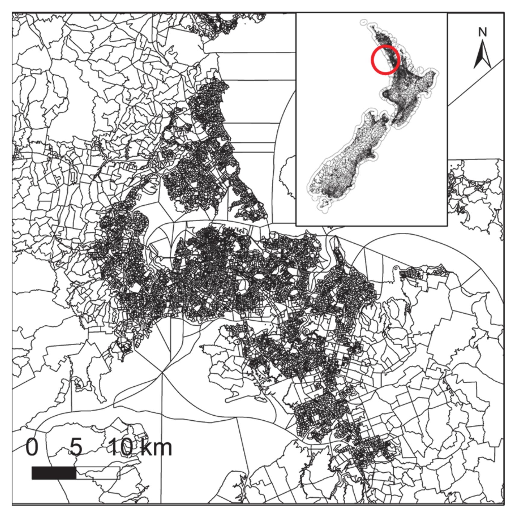
3. Materials and Methods

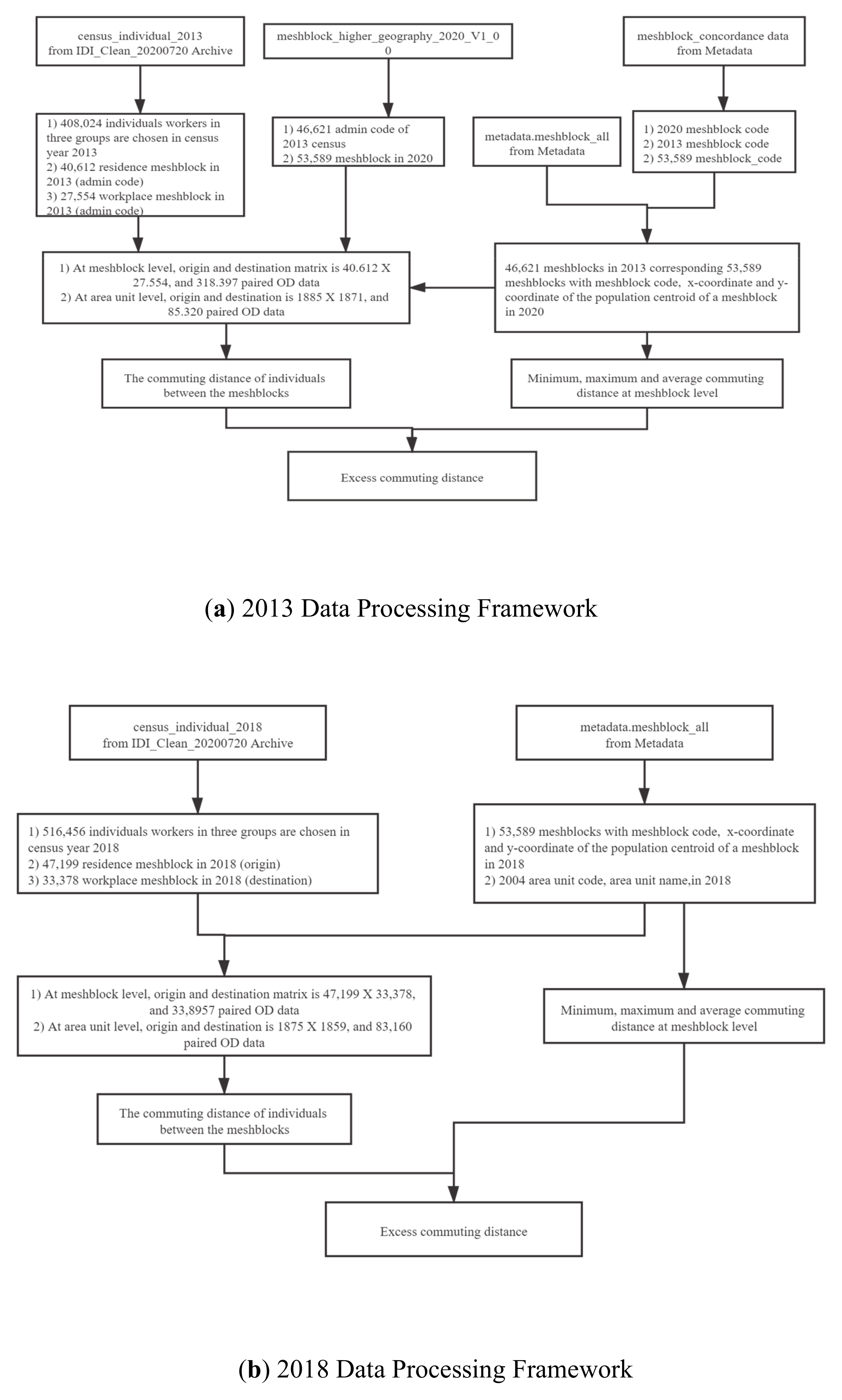
3.1. Integrated Data Infrastructure and the Data Processing

Integrated Data Infrastructure (IDI) is a micro-level dataset about people and households compiled by Statistics New Zealand (Stats NZ) for non-government organisations (NGOs) and academics to gain scientific insight into social issues. The IDI contains person-centred microdata from a wide range of government agencies, surveys, and NGOs [72]. The data can be categorised into eight data categories. This study applies the data from the categories of “people and communities” and “population” to derive the commuting flow of individual workers. These two datasets are generated from the census survey that runs every five years in New Zealand. In this study, the commuting flow of workers is calculated based on the commuting distance between centroids of the residence meshblock and workplace meshblock in the census year of 2013 and 2018. A meshblock is the smallest geographic unit in which the statistical data is reported by Stats NZ [73], similarly to the Census tracts in the United States. There are no more than 120 dwellings within a meshblock.
Figure 1 shows the distribution of meshblocks in Auckland in 2018, the most populous city of New Zealand, which has 1.657 million populations and accounts for 35% of the total population in New Zealand. In Auckland, there were 11,768 meshblocks in 2013 and 13,736 meshblocks in 2018. It is worth noting that Stats NZ significantly reviewed the meshblocks in the 2018 census. This adds another layer of complexity in our data processing. To keep the geographic information consistency, we utilise the meshblock information in 2018 to trace back the corresponding area unit in 2013.
Table 1 shows the sample size of the selected worker groups and meshblocks. There were 203,055 key workers in 2013 and 253,542 key workers in 2018. Two comparison (non-key workers) groups, including finance-insurance and retail trade workers, are introduced. Compared with non-key workers, key workers have a relatively lower turnover rate and work for a particular institution such as hospitals and schools for a more extended period [74]. Thus, because key workers are unlikely to change their workplaces due to the permanency of their employment, they are more sensitive to changes in housing affordability.
Figure 2a,b summarises the data processing within the IDI in 2013 and 2018, respectively. Figure 2a demonstrates the data processing procedure for the census year 2013. From the individual data in the census, the admin codes of meshblocks in 2013 are obtained, and their centroid coordinates are sourced from the concordance metadata. From the datasets, we can calculate each worker’s commuting distance and their excess commuting distance relative to the average commuting distance of the workers living in the same meshblock. Similarly, Figure 2b shows the data processing for the census year 2018. Individual census data and meshblock metadata are employed to collect the residence, workplace meshblock, and corresponding x-y coordinates. The coordinates are used to calculate workers’ commuting distance and excess commuting for 2018.

3.2. Housing Affordability

This study utilises the modified median multiple (housing costs relative to income) as the proxy of housing affordability. When assessing housing affordability, policymakers and researchers have applied the measures such as median multiple ratios, which are price-to-income ratio of the median house price divided by the gross median household income. This indicator has been widely used by the World Bank and Organization for International Cooperation and Development (OECD) [75,76]. In general, the median multiple denotes a ratio of the median house price to the median annual income. Nevertheless, the indicator is sometimes criticised for being oversimplified in measuring housing affordability without taking into account the actual housing costs, especially mortgage expenses. Therefore, in this study, the mortgage rates and loan-to-value (LTV) ratios (i.e., the maximum loan that banks lent to individual) in different census years are used in lieu of the simple median multiple. The formula of our modified median multiple is as follows:
H o u s i n g   U n a f f o r d a b i l i t y a t = H c a t i n c o m e a t
H C a t = p m t m t ¯   r a t e t ,   30 , m e d i a n   p r i c e × L T V t
where Housing Unaffordabilityat is the measurement of unaffordability of the housing at area unit a, in census year t; HCat denotes the housing costs of area unit a, in census year t, while the incomeat is the average annual income of workers living in area unit a in census year t. To measure housing costs, mortgage repayment is used. p m t m t ¯ represents the mean mortgage repayment of meshblocks in an area unit. The numbers 0.050 and 0.057 are used as new two-year residential mortgage interest rates for 2013 and 2018, respectively, and 90% as an LTV ratio to calculate the mortgage repayment of each area unit in 2018. Therefore, the ratio measures the housing unaffordability of a location. The higher the value of Housing Unaffordability, the less affordable the location is.
Table 2 presents a summary of the housing affordability of different regions in Auckland. It is intriguing to note that housing affordability in 2018 and 2013 have a significant difference. Housing unaffordability for 2018 is generally more severe than that in 2013. This indicates that housing affordability in all regions of Auckland has deteriorated between 2013 and 2018. Additionally, housing in Western and Southern Auckland is much more affordable, as manifested by the two lowest housing affordability measures in these regions. In 2013, Central Auckland is the most unaffordable region, followed by the Eastern and Northern regions, while in 2018, the Eastern region is the most unaffordable region, followed by the Central and Northern regions. Apart from the median housing affordability, the minimum and maximum housing affordability vary significantly in Central and Southern Auckland in 2013 and 2018. This indicates that housing affordability is quite diverse across different submarkets.

3.3. Excess Commuting Distance

In essence, estimating excess commuting distances involves two stages of analysis: (1) calculating the actual commuting distance of individuals; and (2) measuring the average commuting distance of particular types of worker who live in the same meshblock. For the first stage, we calculate the actual commuting distance of individuals by using the residence meshblock (r), workplace meshblock (w), and their corresponding x-y coordinates:
D i t = D r w t
D a r o t = 1 N o t D o r t
Equation (3) shows the commuting distance between the residence and workplace meshblock of individuals i at census year t. Equation (4) shows the average commuting distance of one type of workers who live in the same meshblock, where o represents the occupation groups. Thus, Darot denotes the average commuting distance of workers, who work as o occupation at census year t. ∑Dort sums up the commuting distance of workers who are o occupation and live in r meshblock at census year t.
D i e t = D i t D a r o t > 0 , D i t D a o t D i e t = D i t D a r o t < 0 , 0
Equation (5) is employed to determine whether the worker has excess commuting during daily commuting, and further visualises the excess commuting flows. Dit denotes the actual commuting distance of the worker at census year t and obtained from Equation (3), whereas Darot represents the average commuting distance of workers who are in o occupation and live in r meshblock at census year t, where Diet denotes the excess commuting distance of worker at census year t if Diet is larger than zero, and Diet equals zero if Diet is smaller than zero.

4. Results

4.1. Excess Commuting Results for 2013 and 2018

Table 3 presents the commuting flow analyses in 2013 and 2018 for key workers, retail trade workers, and finance-insurance workers. The results show that in 2013, the average commuting distances were 16.61 km, 15.19 km, and 15.53 km for key workers (KEY), retail trade (RET) workers, and finance-insurance workers (FIN), respectively. Evidently, key workers exhibit longer commuting as compared to retail and finance-insurance workers. The minimum commuting distances are zero across three groups as workers can work and live in the same meshblock. The maximum commuting distance is 871.49 km for key workers and 387.91 km for finance-insurance workers, suggesting that there could be “mega-commuters” in these two worker groups.
The average excess commuting distances for key workers, retail trade workers, and finance-insurance workers, respectively, are 8.80 km, 7.64 km, and 8.07 km, respectively. These results imply that the key workers usually commute further than the other two groups.
Apart from the average commuting distance and average excess commuting distance, Table 3 also shows the percentage of excess commuting among each group of workers. The statistics indicate that the percentages of excess commuting for KEY workers, RET workers, and FIN workers are 28.08%, 24.10%, and 25.80%, respectively. This finding suggests that across the three worker groups, key workers suffer the most in terms of excess commuting. Comparing workers in each group, key workers have a higher proportion of workers who suffer excess commuting, whereas fewer finance workers and retail trade workers require excess commuting.
Indeed, in our analysis, it is worth noting that both average commuting distance and excess commuting distance have been reduced from 2013 to 2018 across all occupations. The shorter commutes imply that there is decentralisation of job locations. Together with implementing the Auckland Integrated Fare System (AIFS), which is a smartcard ticketing system that can be used on trains, ferries, and buses since 2011, many infrastructures, such as the electric train service in Eastern and Southern Auckland, were also developed. The construction of Eastern Busway, Manukau and Pah Roads transit lanes and the upgrade of Glenfield Road and Neilson Street altogether improved worker commuting from 2013 to 2018 [77]. Our results suggest that Western Auckland and far Northern and Southern Auckland could be the targeted areas to further develop such infrastructures.
While the results imply that there was an overall reduction in both absolute and excess commuting distance across three groups of workers, key workers are still the group with the disproportionately longest commute among worker groups. The statistics strongly shows that although the absolute commuting distance has been lessened for various workers from 2013 to 2018, key workers are either the most sensitive to deteriorating housing affordability or the most adversely affected by job-housing imbalance.

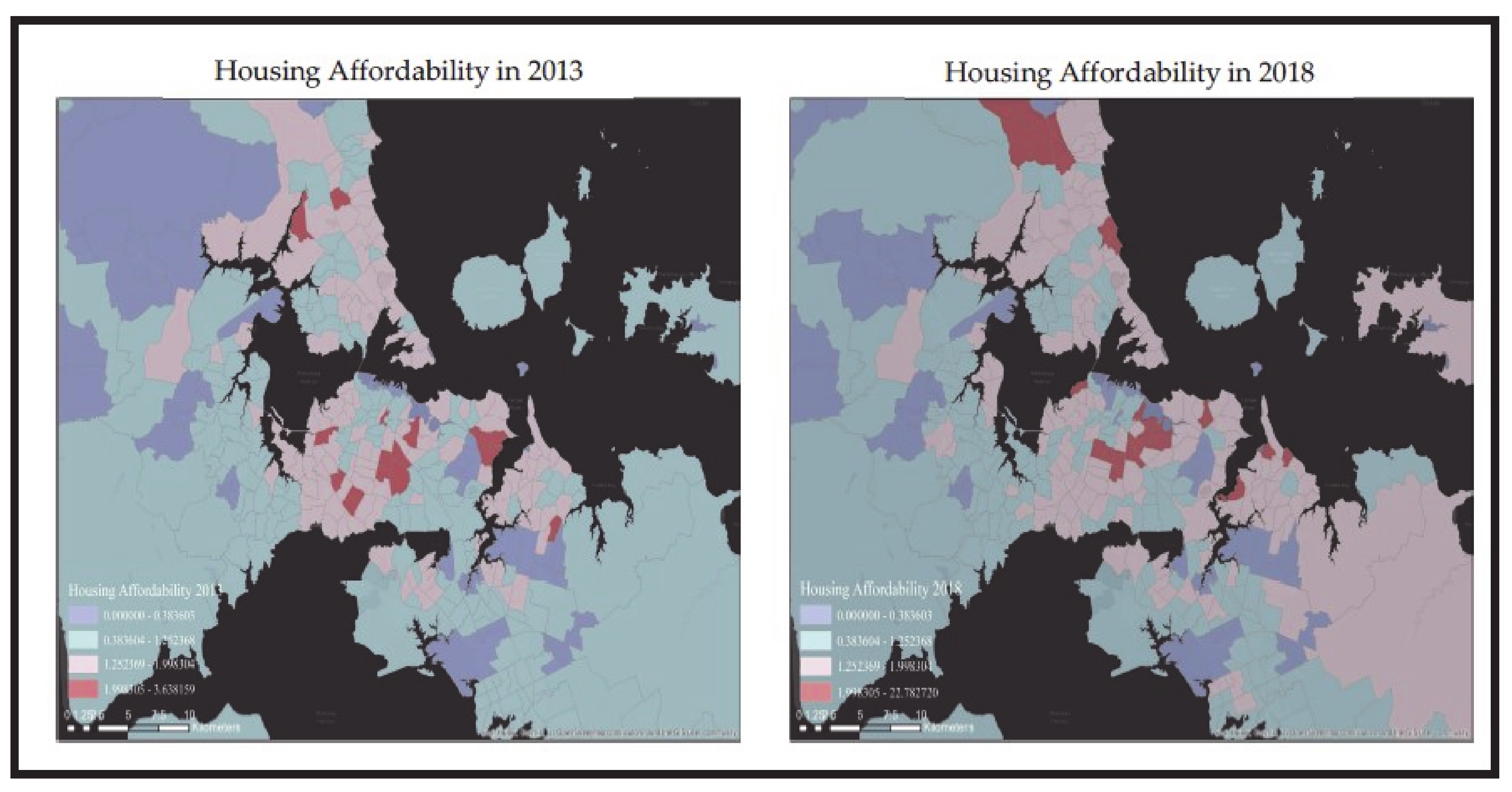
4.2. Housing Affordability in Auckland

Figure 3 illustrates the Auckland Region’s housing affordability in two census years. Both in 2013 and 2018, the deep red coloured areas such as those in Central and Northern Auckland are the least affordable while the purple shaded areas, including Western and Southern Auckland, are the most affordable. The heat map of housing affordability shows that parts of Eastern Auckland became less affordable in 2018. Furthermore, Figure 3 demonstrates that housing affordability deteriorated from 2013 to 2018, since red coloured areas increased in 2018 and the unaffordable areas expanded to Auckland’s outer suburbs.

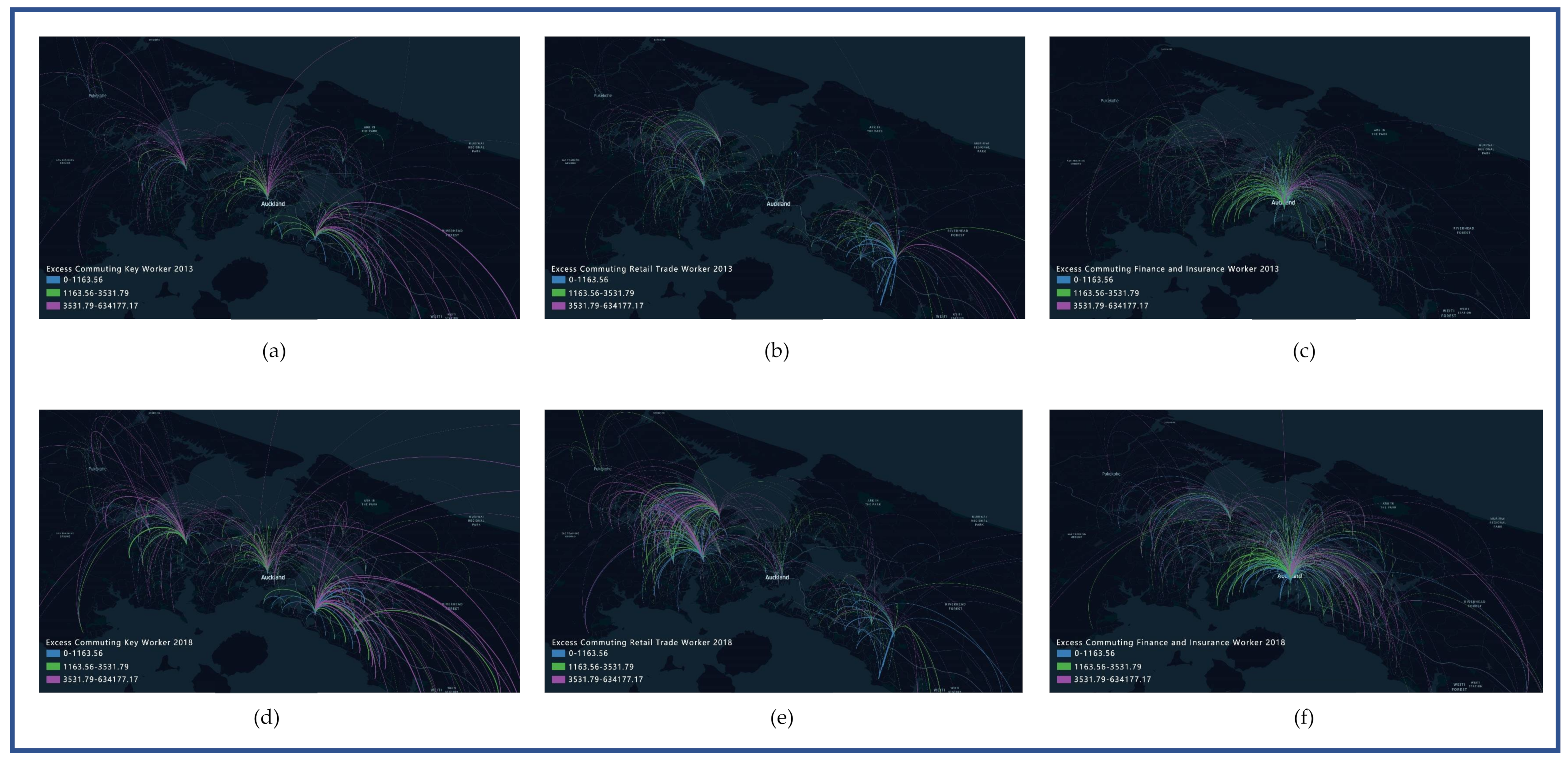
4.3. Visualisation of Excess Commuting Patterns

Figure 4 illustrates the excess commuting flows for three groups of workers in the census years 2013 and 2018. The blue commute flow lines denote an excess commuting distance shorter than 1.16 km, whereas the green line denotes an excess commuting distance between 1.16 km to 3.53 km. The purple flow line denotes an excess commuting distance longer than 3.53 km (1.16 km is the 25 percent tile of excess commuting distance of key workers in 2013, while 3.53 km is the 50 percentile of excess commuting distance of key workers in 2013.).
Figure 4a–c present the excess commuting flows of key workers, retail trade workers, and finance workers in 2013, respectively. As shown in Figure 4a, the commuting flow lines of key workers are dominated by purple coloured lines. The visualised commuting flow suggests that key workers have a relatively longer excess commuting distance and radiate to the fringe of North, South, and Western Auckland. Figure 4b presents the excess commuting flows for the retail trade workers. The blue coloured commuting flow predominates South Auckland, while Central and North Auckland have much green commuting flow strewn around the map. This implies that retail trade workers in South Auckland have relatively minor excess commuting, whereas the magnitude of excess commuting of retail trade workers in North and Central Auckland is slightly more severe. Besides, the less prevalent excess commuting flows for retail trade workers in Central Auckland suggests that the majority of these workers have moderate commuting distances, and can either find a job near their residence or have a sufficient supply of job opportunities. Figure 4c shows the excess commuting flows for finance workers. The commuting pattern indicates that finance workers are more concentrated in the inner city where most banks are located. Most green coloured commuting flows for finance insurance workers are situated between Central and South Auckland, implying that those living in South Auckland require an excess commute to work.
Likewise, Figure 4d–f show the excess commuting flows of the three working groups in 2018. Figure 4d describes the excess commuting flow of key workers, and the purple lines again take over the excess commuting flow in North, South, and Central Auckland. Compared with the map of 2013, there is a noticeable increase in the purple line of key workers and new occurrences of green lines in North and Central Auckland. In addition, more purple lines extend to the city fringe. The visualisation reveals that the magnitude of excess commuting is exacerbated in South and North Auckland over the years. The excess commuting distance of most key workers is more than 3.5 km. Figure 4e shows an excess commuting pattern for retail trade workers and less extensive (green coloured) flows concentrated in South and North Auckland. The pattern implies that many retail trade workers who commute in South and North Auckland have an excess commuting distance of around 1.16 km to 3.53 km. In comparison with the patterns of retail trade workers in 2013, the excess commuting has diminished in South Auckland while worsening in North Auckland.
Figure 4f illustrates the excess commuting flows of finance-insurance workers in 2018, and their excess commuting pattern is similar to the pattern in 2013, which is concentrated in the inner city. Many finance-insurance workers who suffer excess commuting longer than 3.53 km are commuting between Central and Eastern Auckland. Moreover, there is a significant increase of excess commuting between Western and North Auckland among finance workers, and the excess commuting to South Auckland is dispersed to the outer ring.

5. Discussion

5.1. Linking Housing Affordability and Excess Commuting Patterns

As manifested by the housing affordability patterns in Figure 3 and the excess commuting patterns in Figure 4, the excess commuting flow lines became more intensive over the years, regardless of occupation. This implies that the problem of excess commuting is exacerbated. Considering the housing affordability and excess commuting patterns in Auckland over the years, the key workers are the most sensitive to the dynamic of housing affordability, with more deep red coloured areas following the purple coloured commuting flow lines of key workers. The fact that more intensive excess commuting flows of key workers extend to the outer ring of North and South Auckland indicates a severe job-housing imbalance in those areas. In other words, key workers are either unable to find a job near their residence or find it impossible to afford housing near their workplace. As a result, they are pushed out of Central Auckland and forced to undergo excessive commuting.
Interestingly, even though Central Auckland has the most severe housing affordability, the excess commuting of retail workers did not find much concentration, especially in 2013. This means that only a few retail workers in Central Auckland experience excess commuting, and the job-housing balance of retail trade workers is relatively better than that of workers in other occupations. The moderate commuting of retail workers in Central Auckland also translates into sufficient retail trade job opportunities in Central Auckland. Not only are there a variety of part-time and full-time options in Central Auckland, but also there was 52.10% in 2013, while 55.81% in 2018 of retail trade workers were renters. As a result, they have more options in choosing their living and working places. Finance workers are the least sensitive to the housing affordability change since the excess commuting pattern of finance workers radiates from Central Auckland in all directions, regardless of where the unaffordable housing areas are.

5.2. Limitations and Future Work

Despite the contribution discussed, several limitations exist in the current study, mainly due to the strict confidentiality rules for the census data and the limited access to the GIS-related software in the IDI DataLab environment. Due to the protection of personal information, IDI DataLab did not allow researchers to map the road networks to individual addresses. [76] As such, this study can utilise only Euclidean distances as the second-best solution to estimate commuting distances. While some studies using OD cost distance in Auckland [78,79,80,81] have indeed documented the commuting patterns, e.g., Goodyear [78] and Badland et al. [80], their analyses to estimate the commuting distance and time are limited to survey samples. To overcome the limitations of using absolute commuting distance, this study examines the magnitude of “excess” commuting of workers within the same occupation group who live in the same areas and compares their commuting flow and spatial distribution of across multiple occupation groups. Our research provides compelling insights into visualising the commuting flows of different occupation groups in Auckland. The visualisation depicts different patterns of worker mobility of various occupations, as well as corresponding spatial distributions of diverse occupations over the years in the Auckland Region. In addition, the average commuting distances can also be compared with the New Zealand Household Travel Survey estimates [82].
Many previous studies investigated the relationship between the housing market and commuting. The concept of “excess commuting” may not be ground breaking in urban studies [56,57,59,60]. However, the application of excess commuting is rather primitive and confined to measuring job–housing imbalance. Using the concept of excess commuting to improve the measurement of OD seems to be overlooked in the relevant literature, and particularly neglected by the geo-information researchers. First, future research could visualise excess commuting by renters and homeowners across employment groups since renters are more flexible in choosing a residence. Second, researchers can depict the actual commuting flow and benchmark the efficiency of different types of visualisations. Third, the concept of excess commuting can also enrich the measurement of excess commuting through granular-level data. Thus far, limited geo-information studies have explored the commuting patterns and spatial distributions of workers by occupation in Auckland [83]. While Ralphs and Goodyear [83] visualised the commuting flow of all workers in New Zealand at the city level, they failed to demonstrate the degree of deterioration of commuting and of the spatial distribution of workers within a specific city. Future studies could investigate the dynamic of working population mobility by estimating the excess commuting in Auckland longitudinally or by examining policies for alleviating the magnitude of excess commuting and job-housing imbalance.

6. Conclusions

Many studies have addressed the methodological framework for measuring excess commuting and analysing spatial distribution with commuting [65,84,85,86,87]. This study utilises GIS framework and the IDI data at the individual level to examine how excess commuting is associated with deteriorating housing affordability. The use of spatial information in the IDI data is novel, and the methodology of visualising excess commuting is also an innovative way to present commuting flows. The visualisation of this study suggests that although the overall commuting distance and excess commuting steadily reduced from the year 2013 to 2018 due to either the decentralisation of job opportunities and/or the improvement of public transportation, key workers who usually work in a fixed location continue to suffer the longest commutes and exhibit disproportionate excess commuting relative to other workers. Compared to the other two major groups of workers in Auckland, constrained by budget key workers are making sub-optimal housing choices living further away from where they work and accepting longer commutes.
To the best of our knowledge, few studies are examining excess commuting from an occupation perspective. Theoretically, this study fills the research gap in commuting literature by considering the roles of occupations in the context of commuting patterns and spatial distributions. Our excess origin-destination (OD) flow model, estimating average commuting distances and average excess commuting distances, shows that the commuting flow patterns vary by occupations. Moreover, this study shows that key workers suffer the lengthiest commutes and have the longest excess commuting despite the reduced commutes across other worker groups. It is due to the fact that there is an increasing trend of key workers living in the outer ring of the Auckland Region and residing much more dispersed.
Practically, this study introduces a novel concept of using excess commuting flows in visualising the conventional presentation of commuting flows. The proposed method also represents a new approach to alleviating the cluttering problem when visualising the commute flow maps at an individual level. First, using excess commuting flow rather than actual commuting flow can streamline the flow lines on the map without missing the crucial information from the raw data. Such “excess commuting flow” visualisation can be applied to urban studies on commute flows in the future. Second, by quantifying excess commute in different occupations, policymakers can be better informed to formulate a city structure that assuages excess commute. Creating more affordable houses nearby job centres and decentralising workplaces to make the job centres more accessible are always the key in alleviating the excess commuting issue, no matter in New Zealand or elsewhere in the world.

Author Contributions

Conceptualisation, Chuyi Xiong and Ka Shing Cheung; methodology, Chuyi Xiong and Ka Shing Cheung; software, Chuyi Xiong; validation, Chuyi Xiong and Ka Shing Cheung; formal analysis, Chuyi Xiong; investigation, Ka Shing Cheung; resources, Chuyi Xiong; data curation, Chuyi Xiong and Ka Shing Cheung; writing—original draft preparation, Chuyi Xiong and Ka Shing Cheung; writing—review and editing, Chuyi Xiong, Ka Shing Cheung, and Olga Filippova; visualisation, Chuyi Xiong; supervision, Ka Shing Cheung and Olga Filippova; project administration, Chuyi Xiong; funding acquisition, Ka Shing Cheung and Olga Filippova. All authors have read and agreed to the published version of the manuscript.

Funding

This research project was financially supported by the Ministry of Business, Innovation and Employment, New Zealand National Science Challenge: Building Better Homes Towns and Cities (BBHTC). The APC was funded by Performance-Based Research Fund (PBRF), New Zealand Tertiary Education Commission (TEC).

Institutional Review Board Statement

Not applicable.

Informed Consent Statement

Not applicable.

Acknowledgments

We would like to thank Eileen Li for her excellent research assistance on this project to help compile part of the Integrated data infrastructure (IDI) by Stats NZ.

Conflicts of Interest

The authors declare no conflict of interest.

References

  1. Banister, D. Unsustainable Transport: City Transport in the New Century; Routledge: Oxfordshire, UK, 2005. [Google Scholar]
  2. Cropper, M.L.; Gordon, P.L. Wasteful commuting: A re-examination. J. Urban Econ. 1991, 29, 2–13. [Google Scholar] [CrossRef]
  3. Ta, N.; Chai, Y.; Zhang, Y.; Sun, D. Understanding job-housing relationship and commuting pattern in Chinese cities: Past, present and future. Transp. Res. Part D Transp. Environ. 2017, 52, 562–573. [Google Scholar] [CrossRef]
  4. Kain, J.F. Housing segregation, negro employment, and metropolitan decentralization. Q. J. Econ. 1968, 82, 175–197. [Google Scholar] [CrossRef]
  5. Kain, J.F. The spatial mismatch hypothesis: Three decades later. Hous. Policy Debate 1992, 3, 371–460. [Google Scholar] [CrossRef]
  6. Steele, A.; Todd, S. New developments for key worker housing in the UK. Struct. Surv. 2004, 22, 179–189. [Google Scholar] [CrossRef]
  7. Morrison, N. Assessing the need for key-worker housing: A case study of Cambridge. Town Plan. Rev. 2003, 74, 281–300. [Google Scholar] [CrossRef]
  8. Batty, M.; Murcio, R.; Iacopini, I.; Vanhoof, M.; Milton, R. London in lockdown: Mobility in the pandemic city. In COVID-19 Pandemic, Geospatial Information, and Community Resilience; CRC Press: Boca Raton, FL, USA, 2021; pp. 229–244. [Google Scholar]
  9. Weaver, M. Key worker housing: The issue explained. Guardian 2004, 25, 4. Available online: https://www.theguardian.com/society/2004/may/25/keyworkerhousing (accessed on 26 April 2021).
  10. Airey, J.; Wales, R. Revitalising Key Worker Housing; Policy Exchange: London, UK, 2019. [Google Scholar]
  11. Morrison, N. Reinterpreting the key worker problem within a university town: The case of Cambridge, England. Town Plan. Rev. 2013, 84, 721–743. [Google Scholar] [CrossRef]
  12. Morrison, N.; Monk, S. Job-housing mismatch: Affordability crisis in Surrey, South East England. Environ. Plan A 2006, 38, 1115–1130. [Google Scholar] [CrossRef]
  13. Wilson, Z. Cost of Auckland Living Pushing People out to Whanganui. NZ Herald 18 February 2018. Available online: https://www.nzherald.co.nz/nz/cost-of-auckland-living-pushing-people-out-to-whanganui/2RG7ND4Z64M5P7Q2FIA34SAH3U/ (accessed on 10 May 2021).
  14. Mandic, S.; Jackson, A.; Lieswyn, J.; Mindell, J.S.; García Bengoecheak, E.; Spence, J.C.; Coppell, K.; Wade-Brown, C.; Wooliscroft, B.; Hinckson, E. Development of key policy recommendations for active transport in New Zealand: A multi-sector and multidisciplinary endeavour. J. Transp. Health 2020, 18, 100859. [Google Scholar] [CrossRef]
  15. Stroombergen, A.; Bealing, M.; Torshizian, E.; Poot, J. Impacts of Socio-Demographic Changes on the New Zealand Land Transport System; NZ Transport Agency: Waikato, New Zealand, 2018. [Google Scholar]
  16. Deng, M.; Xie, L.; Lin, X. An analysis on the characteristics of the trips of Guangzhou inhabitants and development of urban communications. Trop. Geogr. 2000, 20, 37–41. [Google Scholar]
  17. Li, C.; Chai, Y. A study on the commuting features of Dalian citizens. Hum. Geogr. 2000, 15, 67–72. [Google Scholar]
  18. Schwanen, T.; Dijst, M. Travel-time ratios for visits to the workplace: The relationship between commuting time and work duration. Transp. Res. Part A Policy Pract. 2002, 36, 573–592. [Google Scholar] [CrossRef]
  19. Chai, Y. Urban Structure Comparison between China and Japan; Peking University Press: Beijing, China, 1999. [Google Scholar]
  20. Zhou, S.; Yang, L. Study on the spatial characteristic of commuting in Guangzhou. Urban Transp. China 1 2005, 3, 62–67. [Google Scholar] [CrossRef]
  21. Coombes, M. Defining labour market areas by analysing commuting data: Innovative methods in the 2007 review of travel-to-work areas. In Technologies for Migration and Commuting Analysis: Spatial Interaction Data Applications; IGI Global: Hershey, PA, USA, 2010; pp. 227–241. [Google Scholar]
  22. Hincks, S. Daily interaction of housing and labour markets in north west England. Reg. Stud. 2012, 46, 83–104. [Google Scholar] [CrossRef]
  23. Hincks, S.; Wong, C. The spatial interaction of housing and labour markets: Commuting flow analysis of north west England. Urban Stud. 2010, 47, 620–649. [Google Scholar] [CrossRef] [Green Version]
  24. Zhao, P.; Lü, B.; de Roo, G. Impact of the jobs-housing balance on urban commuting in Beijing in the transformation era. J. Transp. Geogr. 2011, 19, 59–69. [Google Scholar] [CrossRef]
  25. Weber, J.; Sultana, S. Employment sprawl, race and the journey to work in Birmingham, Alabama. Southeast. Geogr. 2008, 48, 53–74. [Google Scholar] [CrossRef]
  26. Crane, R.; Chatman, D. Traffic and Sprawl: Evidence from US Commuting from 1985–1997; University of Southern California: Los Angeles, CA, USA, 2003; Volume 6. [Google Scholar]
  27. Ma, Y.; Xu, W.; Zhao, X.; Li, Y. Modeling the hourly distribution of population at a high spatiotemporal resolution using subway smart card data: A case study in the central area of Beijing. ISPRS Int. J. Geo-Inf. 2017, 6, 128. [Google Scholar] [CrossRef] [Green Version]
  28. Wu, H.; Liu, L.; Yu, Y.; Peng, Z.; Jiao, H.; Niu, Q. An agent-based model simulation of human mobility based on mobile phone data: How commuting relates to congestion. ISPRS Int. J. Geo-Inf. 2019, 8, 313. [Google Scholar] [CrossRef] [Green Version]
  29. Chen, X.; Guo, S.; Yu, L.; Hellinga, B. Short-term forecasting of transit route OD matrix with smart card data. In Proceedings of the 2011 14th International IEEE Conference on Intelligent Transportation Systems (ITSC), Washington, DC, USA, 5–7 October 2011; pp. 1513–1518. [Google Scholar]
  30. Toqué, F.; Côme, E.; Mahrsi, M.K.E.; Oukhellou, L. Forecasting dynamic public transport origin-destination matrices with long-short term memory recurrent neural networks. In Proceedings of the 2016 IEEE 19th International Conference on Intelligent Transportation Systems (ITSC), Rio de Janeiro, Brazil, 1–4 November 2016; Available online: https://ieeexplore.ieee.org/stamp/stamp.jsp?arnumber=7795689 (accessed on 30 June 2021).
  31. Yeghikyan, G.; Opolka, F.L.; Nanni, M.; Lepri, B.; Lì, P. Learning mobility flows from urban features with spatial interaction models and neural networks. In Proceedings of the 2020 IEEE International Conference on Smart Computing (SMARTCOMP), Bologna, Italy, 14–17 September 2020. [Google Scholar]
  32. Zhou, J.; Murphy, E.; Long, Y. Commuting efficiency in the Beijing metropolitan area: An exploration combining smartcard and travel survey data. J. Transp. Geogr. 2014, 41, 175–183. [Google Scholar] [CrossRef] [Green Version]
  33. Ma, X.; Liu, C.; Wen, H.; Wang, Y.; Wu, Y.J. Understanding commuting patterns using transit smart card data. J. Transp. Geogr. 2017, 58, 135–145. [Google Scholar] [CrossRef]
  34. Yang, X.; Fang, Z.; Yin, L.; Li, J.; Zhou, Y.; Lu, S. Understanding the spatial structure of urban commuting using mobile phone location data: A case study of Shenzhen, China. Sustainability 2018, 10, 1435. [Google Scholar] [CrossRef] [Green Version]
  35. Zhou, J.; Murphy, E.; Long, Y. Commuting efficiency gains: Assessing different transport policies with new indicators. Int. J. Sustain. Transp. 2019, 13, 710–721. [Google Scholar] [CrossRef]
  36. Guo, D. Flow mapping and multivariate visualization of large spatial interaction data. IEEE Trans. Vis. Comput. Graph. 2009, 15, 1041–1048. [Google Scholar]
  37. Lu, M.; Liang, J.; Wang, Z.; Yuan, X. Exploring OD patterns of interested region based on taxi trajectories. J. Vis. 2016, 19, 811–821. [Google Scholar] [CrossRef]
  38. Ni, B.; Shen, Q.; Xu, J.; Qu, H. Spatio-temporal flow maps for visualizing movement and contact patterns. Vis. Inform. 2017, 1, 57–64. [Google Scholar] [CrossRef]
  39. Rowe, F.; Patias, N. Mapping the spatial patterns of internal migration in Europe. Reg. Stud. Reg. Sci. 2020, 7, 390–393. [Google Scholar] [CrossRef]
  40. Dong, W.; Wang, S.; Chen, Y.; Meng, L. Using eye tracking to evaluate the usability of flow maps. ISPRS Int. J. Geo-Inf. 2018, 7, 281. [Google Scholar] [CrossRef] [Green Version]
  41. Sakamanee, P.; Phithakkitnukoon, S.; Smoreda, Z.; Ratti, C. Methods for inferring route choice of commuting trip from Mobile phone network data. ISPRS Int. J. Geo-Inf. 2020, 9, 306. [Google Scholar] [CrossRef]
  42. Tobler, W.R. Experiments in migration mapping by computer. Am. Cartogr. 1987, 14, 155–163. [Google Scholar] [CrossRef] [Green Version]
  43. Rae, A. From spatial interaction data to spatial interaction information? Geovisualisation and spatial structures of migration from the 2001 UK census. Comput. Environ. Urban Syst. 2009, 33, 161–178. [Google Scholar] [CrossRef]
  44. Vale, D.S.; Pereira, M.; Viana, C.M. Different destination, different commuting pattern? Analyzing the influence of the campus location on commuting. J. Transp. Land Use 2018, 11, 1–18. [Google Scholar] [CrossRef] [Green Version]
  45. Van Acker, V.; Witlox, F. Commuting trips within tours: How is commuting related to land use? Transportation 2011, 38, 465–486. [Google Scholar] [CrossRef]
  46. Yang, F.; Jin, P.J.; Cheng, Y.; Zhang, J.; Ran, B. Origin-destination estimation for non-commuting trips using location-based social networking data. Int. J. Sustain. Transp. 2015, 9, 551–564. [Google Scholar] [CrossRef]
  47. Möller, C.; Alfredsson-Olsson, E.; Ericsson, B.; Overvåg, K. The border as an engine for mobility and spatial integration: A study of commuting in a Swedish-Norwegian context. Nor. Geogr. Tidsskr. J. Geogr. 2018, 72, 217–233. [Google Scholar] [CrossRef]
  48. Zhang, S.; Tang, J.; Wang, H.; Wang, Y.; An, S. Revealing intra-urban travel patterns and service ranges from taxi trajectories. J. Transp. Geogr. 2017, 61, 72–86. [Google Scholar] [CrossRef]
  49. Watson, J.R.; Prevedouros, P.D. Derivation of origin—Destination distributions from traffic counts: Implications for freeway simulation. Transp. Res. Rec. 2006, 1964, 260–269. [Google Scholar] [CrossRef]
  50. Kreindler, G.E.; Miyauchi, Y. Measuring Commuting and Economic Activity Inside Cities with Cell Phone Records; National Bureau of Economic Research: Cambridge, MA, USA, 2021. [Google Scholar]
  51. Guo, D.; Zhu, X. Origin-destination flow data smoothing and mapping. IEEE Trans. Vis. Comput. Graph. 2014, 20, 2043–2052. [Google Scholar] [CrossRef] [PubMed]
  52. Andrienko, G.; Andrienko, N. A general framework for using aggregation in visual exploration of movement data. Cartogr. J. 2010, 47, 22–40. [Google Scholar] [CrossRef] [Green Version]
  53. Massey, D.; Denton, N.A. American Apartheid: Segregation and the Making of the Underclass; Harvard University Press: Cambridge, MA, USA, 1993. [Google Scholar]
  54. Hamilton, B.W.; Röell, A. Wasteful commuting. J. Polit. Econ. 1982, 90, 1035–1053. [Google Scholar] [CrossRef]
  55. Alonso, W. Location and Land Use: Toward a General Theory of Land Rent; Harvard University Press: Cambridge, MA, USA, 1964. [Google Scholar]
  56. Mills, E.S. An aggregative model of resource allocation in a metropolitan area. Am. Econ. Rev. 1967, 57, 197–210. [Google Scholar]
  57. Muth, R.F. Cities and Housing: The Spatial Pattern of Urban Residential Land Use; Cambridge University Press: Cambridge, UK, 1969. [Google Scholar]
  58. Small, K.A.; Song, S. “Wasteful” commuting: A resolution. J. Polit. Econ. 1992, 100, 888–898. [Google Scholar] [CrossRef]
  59. Hamilton, B.W. Wasteful commuting again. J. Polit. Econ. 1989, 97, 1497–1504. [Google Scholar] [CrossRef]
  60. White, M.J. Urban commuting journeys are not “wasteful”. J. Polit. Econ. 1988, 96, 1097–1110. [Google Scholar] [CrossRef]
  61. Giménez, J.I.; Molina, J.A.; Velilla, J. Excess Commuting in the US: Differences Between the Self-Employed and Employees; IZA DP No. 9425; Institute of Labor Economics (IZA): Bonn, Germany, 2015. [Google Scholar]
  62. Ha, J.; Lee, S.; Kwon, S.M. Revisiting the relationship between urban form and excess commuting in US metropolitan areas. J. Plan. Educ. Res. 2018, 0739456X18787886. [Google Scholar] [CrossRef]
  63. Bwire, H.; Zengo, E. Comparison of efficiency between public and private transport modes using excess commuting: An experience in Dar es Salaam. J. Transp. Geogr. 2020, 82, 102616. [Google Scholar] [CrossRef]
  64. Park, C.; Chang, J.S. Transportation planning and technology spatial equity of excess commuting by transit in seoul spatial equity of excess commuting by transit in Seoul. Transp. Plan. Technol. 2019, 43, 101–112. [Google Scholar] [CrossRef]
  65. Horner, M.W. Extensions to the concept of excess commuting. Environ. Plan. A Econ. Sp. 2002, 34, 543–566. [Google Scholar] [CrossRef]
  66. Murphy, E.; Killen, J.E. Commuting economy: An alternative approach for assessing regional commuting efficiency. Urban Stud. 2011, 48, 1255–1272. [Google Scholar] [CrossRef]
  67. O’Kelly, M.E.; Niedzielski, M.A. Efficient spatial interaction: Attainable reductions in metropolitan average trip length. J. Transp. Geogr. 2008, 16, 313–323. [Google Scholar] [CrossRef]
  68. Merriman, D.; Ohkawara, T.; Suzuki, T. Excess commuting in the Tokyo metropolitan area: Measurement and policy simulations. Urban Stud. 1995, 32, 69–85. [Google Scholar] [CrossRef]
  69. O’Kelly, M.E.; Lee, W. Disaggregate journey-to-work data: Implications for excess commuting and jobs–housing balance. Environ. Plan. A 2005, 37, 2233–2252. [Google Scholar] [CrossRef]
  70. Kim, S. Excess commuting for two-worker households in the Los Angeles metropolitan area. J. Urban Econ. 1995, 38, 166–182. [Google Scholar] [CrossRef] [Green Version]
  71. Frost, M.; Linneker, B.; Spence, N. Excess or wasteful commuting in a selection of British cities. Transp. Res. Part A Policy Pract. 1998, 32, 529–538. [Google Scholar] [CrossRef]
  72. Integrated Data Infrastructure; Stats NZ: Wellingon, New Zealand; New Zealand Government: New Zealand. 2021. Available online: https://www.stats.govt.nz/integrated-data/integrated-data-infrastructure/ (accessed on 15 April 2021).
  73. 2018 Census Data User Guide, 2nd ed.; Stats NZ: Wellington, New Zealand, 2021.
  74. New Zealand Staff Turnover Survey Report 2018; Lawson Williams: Auckland, New Zealand, 2018.
  75. Moss, M.L.; Qing, C. The Emergence of the “Super-Commuter”; Rudin Center for Transportation & Management: New York, NY, USA, 2012. [Google Scholar]
  76. Microdata Output Guide, 5th ed. Stats NZ: Wellington, New Zealand. 2016. Available online: https://www.stats.govt.nz/assets/Methods/Microdata-Output-Guide-2020-v5-1.pdf (accessed on 29 April 2021).
  77. Auckland Transport. Projects & Roadworks. Available online: https://at.govt.nz/projects-roadworks (accessed on 28 April 2021).
  78. Goodyear, R. Workforces on the move: An examination of commuting patterns to the cities of Auckland, Wellington and Christchurch. In Proceedings of the NZAE Conference, Willington City, New Zealand, 9–11 July 2008. [Google Scholar]
  79. Mattingly, K.; Morrissey, J. Housing and transport expenditure: Socio-spatial indicators of affordability in Auckland. Cities 2014, 38, 69–83. [Google Scholar] [CrossRef]
  80. Badland, H.M.; Schofield, G.M.; Schluter, P.J. Objectively measured commute distance: Associations with actual travel modes and perceptions to place of work or study in Auckland, New Zealand. J. Phys. Act. Heal. 2007, 4, 80–86. [Google Scholar] [CrossRef] [PubMed] [Green Version]
  81. Australasian Railway Association. The Costs of Commuting: An Analysis of Potential Commuter Savings; Australasian Railway Association: Canberra, Australia, 2015. [Google Scholar]
  82. Ministry of Transport. New Zealand Household Travel Survey: Travel to Work, by Main Urban Area Results (3-Year Moving Average). Available online: http://nzdotstat.stats.govt.nz/wbos/Index.aspx?DataSetCode=TABLECODE7432 (accessed on 17 June 2021).
  83. Ralphs, M.; Goodyear, R. The daily commute: An analysis of the geography of the labour market using 2006 Census data. Labour Employ. Work New Zeal. 2008. [Google Scholar] [CrossRef]
  84. Charron, M. From excess commuting to commuting possibilities: More extension to the concept of excess commuting. Environ. Plan. A 2007, 39, 1238–1254. [Google Scholar] [CrossRef]
  85. Ma, K.-R.; Banister, D. Urban spatial change and excess commuting. Environ. Plan. A 2007, 39, 630–646. [Google Scholar] [CrossRef]
  86. Murphy, E. Excess commuting and modal choice. Transp. Res. Part A Policy Pract. 2009, 43, 735–743. [Google Scholar] [CrossRef]
  87. Ahlfeldt, G.M.; Redding, S.J.; Sturm, D.M.; Wolf, N. The economics of density: Evidence from the Berlin Wall. Econometrica 2015, 83, 2127–2189. [Google Scholar] [CrossRef] [Green Version]
Figure 1. Distribution of meshblocks in Auckland in 2018.
Ijgi 10 00457 g001
Figure 2. (a) and (b). Excess commuting data process framework by using IDI data for 2013 and 2018.
Ijgi 10 00457 g002
Figure 3. Housing affordability in Auckland.
Ijgi 10 00457 g003
Figure 4. (af). Excess commuting patterns in 2013 and 2018. Figure (ac) and Figure (df) illustrated the excess commuting for key workers, retail trade workers and finance and insurance workers in 2013 and 2018, respectively. Notes: The flow diagram is also available online, retrieved from http://cdn-imgjpg.test.upcdn.net/2021/06/17/1ORojfm3.png (accessed on 29 April 2021). To maintain privacy, confidentiality, and data security, Stats NZ will suppress the information from IDI (remove its value) when it releases its data outputs. Thus, we can only use the commuting data of the meshblocks with more than six workers living in a meshblock. The detailed microdata output guide can be retrieved from https://www.stats.govt.nz/assets/Uploads/Integrated-data-infrastructure/microdata-output-guide-fourth-edition.pdf (accessed on 29 April 2021).
Ijgi 10 00457 g004
Table 1. Census sample size.
Occupation ClassificationOccupation Code (First Three-Digit)20132018
Key workersSchool Teachers24177,58094,509
Nursing25441,37951,591
Health Workers41118,22829,229
Child Carers4218,66710,548
Personal Carers42341,33748,663
Fire Fighters and Police44115,86419,002
Total 203,055253,542
Finance-Insurance workersAccountants and Auditors22128,14333,999
Financial Brokers and Dealers22210,47312,507
Insurance Agents61143,53355,476
Total 82,149101,982
Retail Trade workersSalespersons62196,834125,313
Sales Support Workers6398,1729,009
Storepersons74117,81426,610
Total 122,820160,932
Meshblock Residence 40,61247,199
Meshblock Workplace 27,55433,378
Paired Meshblock 318,397338,957
Notes: The IDI of Statistics New Zealand provides the meshblock codes and area unit codes of residence and workplace of each individual with their x-y coordinates and occupation codes. The key workers group, finance-insurance workers, and retail trade workers reported 40,612 residence meshblocks and 27,554 workplace meshblocks in 2013, and they reported 47,199 residence meshblocks and 33,378 workplace meshblocks in 2018. 318,397 paired origin (residence meshblock)–destination (workplace meshblock) flows were found in 2013 while 338,957 paired OD flows were found in 2018. Those meshblock flows can aggregate to 85,320 area unit flows in 2013 and 83,160 area unit flows in 2018.
Table 2. Summary of housing affordability in Auckland.
20132018
RegionMinMedianMaxMinMedianMax
Northern0.7701.2272.4210.6491.2613.690
Western0.7751.0311.3060.8541.0521.375
Central0.3081.4013.4380.2161.4092.796
Eastern0.7231.3942.1081.0441.4822.296
Southern0.3841.0063.6380.3381.06922.783
Table 3. Commuting distance pattern by occupation in 2013 and 2018.
OccupationCommuting Distance (km)Excess Commuting (km)Excess Commuting (%)
2013MeanMinMaxMean%
KEY workers16.610.00871.498.8028.08%
RET workers15.190.0051.397.6424.10%
FIN workers15.530.00387.918.0725.80%
2018MeanMinMaxMean%
KEY workers13.500.00561.646.1031.35%
RET workers12.330.0059.885.9826.97%
FIN workers12.440.00525.095.8729.74%
Note: The distances are all the direct distance between the residence and centroid of workplace meshblock.
Publisher’s Note: MDPI stays neutral with regard to jurisdictional claims in published maps and institutional affiliations.

