Improving Victimization Risk Estimation: A Geographically Weighted Regression Approach

Abstract

Standardized crime rates (e.g., “homicides per 100,000 people”) are commonly used in crime analysis as indicators of victimization risk but are prone to several issues that can lead to bias and error. In this study, a more robust approach (GWRisk) is proposed for tackling the problem of estimating victimization risk. After formally defining victimization risk and modeling its sources of uncertainty, a new method is presented: GWRisk uses geographically weighted regression to model the relation between crime counts and population size, and the geographically varying coefficient generated can be interpreted as the victimization risk. A simulation study shows how GWRisk outperforms naïve standardization and Empirical Bayesian Estimators in estimating risk. In addition, to illustrate its use, GWRisk is applied to the case of residential burglaries in Belo Horizonte, Brazil. This new approach allows more robust estimates of victimization risk than other traditional methods. Spurious spikes of victimization risk, commonly found in areas with small populations when other methods are used, are filtered out by GWRisk. Finally, GWRisk allows separating a reference population into segments (e.g., houses, apartments), estimating the risk for each segment even if crime counts were not provided per segment.

1. Introduction

Reliable maps are an important component for understanding crime and planning solutions. While in some cases raw crime counts per location may be sufficient, estimating standardized rates (e.g., “homicides per 100,000 people” or “burglaries per 1000 residences”) might be useful for cross comparing crime between different regions, since this standardized rate can be interpreted as an estimate of victimization risk per individual. This type of estimation, however, comes with a number of challenges that, if not addressed, could lead to biased or error-prone estimates. These challenges include: choosing an appropriate reference population (e.g., should we consider burglaries per residence, burglaries per resident, or maybe even burglaries per offender?); bias and error in the reference population, and handling small reference populations. While some of these challenges have in the past been addressed individually by other studies, an integrated exploration on how to handle all of these issues is still lacking.

In this study, these sources of uncertainty to risk estimation are integrated into a mathematical framework and a new and more robust approach is proposed for tackling these issues. This new approach, referred to here as the GWRisk method, employs Geographically Weighted Regression, in which the estimated victimization risks are obtained from the fitted geographically varying regression coefficients. The method allows multiple segments of a reference populations to be used (e.g., different age groups, or different housing types), estimating separate risks for each segment even if crime counts are not available per population segment. Through a controlled simulated study, a comparison is made between the GWRisk method and other traditional methods of standardization (e.g., simple division, Empirical Bayesian Estimators), with the new method providing better estimates for victimization risks. In addition, to illustrate its use, the method is applied to a real-world dataset, using residential burglaries from the city of Belo Horizonte, Brazil. Therefore, the new method not only is capable of providing more reliable crime maps, but also represents a novel use of Geographically Weighted Regression.

This paper is organized as follows. The remainder of this Introduction section describes the previous research on the topic, focusing first on crime standardization and then on geographically weighted regression. The Materials and Methods section starts by mathematically formulating the different sources of uncertainty in victimization risk (Section 2.1), then proceeding with a description of the new method for estimating risk (Section 2.2). The validation study for this new method is described in Section 2.3, and the application study is described in Section 2.4. Finally, the results of the validation and application studies are shown in the Results section, and the contribution of this paper is discussed and summarized in the Discussion section.

1.1. Literature on Crime Standardization and the Estimation of Victimization Risk

There are many different challenges involved in estimating accurate victimization risks, including issues of data quality, choice of an adequate reference population and issues arising from dealing with small populations. Although these issues have been explored to some extent by previous research, an integration of these issues is still lacking, and reliable estimation of victimization risk remains a challenge.

Issues on the reliability of the data have been called the “dark figure of crime” [1,2]; in other words, how much do police registers and other official records faithfully represent the real distribution of crime? Victimization surveys can be used to estimate this dark figure and mitigate its effects. Research has been done on the different underreporting rates for different crimes—property crimes such as burglary and auto theft are more likely to be reported, while crimes of a more personal nature such as sexual and domestic violence have high rates of underreporting [3]. These surveys, however, tend to be costly [4,5], and are usually available only at broad geographical scales (e.g., per city, county, state, or country).

Another issue when estimating victimization risk is choosing an appropriate reference population, also known as the “denominator dilemma” [6]. The work of Boggs [7] is usually considered to be the first to more systematically investigate the problem of choosing a reference population, and a more recent review of different approaches is provided by Solymosi et al. [8]. For instance, using reference populations other than resident population has been suggested by different authors, such as number of households for burglary [9], and number of vehicles for vehicle theft [10]. Solymosi et al. [8] compare the use of different reference populations for calculating victimization risk, while in Pettiway [11], the presence of multiple candidates for reference population was tackled by calculating a composite index from the individual datasets. Finally, advances in technological tools and data availability (e.g., remote sensing, simulation models, Twitter data) have enabled the estimation of the ambient population at specific places and times of the day through multiple approaches [12,13,14,15,16].

Although victimization surveys and improved methods for estimating ambient population contribute to more accurate estimates of victimization risk, even small errors can create significant distortions for naïve standardization if the reference population is small. This is particularly relevant considering the growing interest in mapping crime at fine geographic units [17,18,19].

As such, more sophisticated techniques may be required to produce reliable victimization risk estimates, but this issue has been relatively less examined in the literature. Kafadar [20] proposed a method of spatial smoothing for dealing with similar issues of uncertainty when calculating rates of cancer risk, which was then applied by Anselin et al. [21] in a crime analysis application. Empirical Bayesian Estimation has been used in several studies [21,22,23] to deal with unstable rates in small populations. Finally, regression techniques (often following Bayesian approaches) have been applied to estimate risk not only for crime [24,25] but for other types of events such as diseases and accidents [26,27,28,29,30]. These approaches have some similarities to the methodology proposed in this paper; nevertheless, there are significant differences in how risk is defined and modeled, as well as how spatial dependence is treated. In particular, I have found no study employing Geographically Weighted Regression as a strategy for risk estimation; I also found no method in which multiple segments of a reference population were used, generating separate estimated risks for each segment (e.g., separate estimated risks for houses and for apartments, when dealing with burglaries).

1.2. Literature on Geographically Weighted Regression

Geographically Weighted Regression (GWR) is a local regression technique in which the regression coefficients are allowed to vary in space, being estimated at different locations on a moving-window style in which the size of the window is determined by bandwidth parameter [31,32]. The method has been widely used in spatial analysis as a way to measure and model the non-stationarity of processes, that is, the possibility that the investigated link between a dependent variable and its explanatory factors varies in space [33,34,35]. The model has been further expanded into more complex and general variants, such as Geographically and Temporally Weighted Regression (GTWR, see Huang et al. [36]), Multiscale Geographically Weighted Regression (MGWR, see Fotheringham et al. [37]) and Multiscale Geographically and Temporally Weighted Regression (MGTWR, see Wu et al. [38]). In GTWR, the regressed coefficients are allowed to vary in time as well as in space; in MGWR, the bandwidth is allowed to be different for each coefficient considered; finally, MGTWR is a combination of the former two. In this paper, the standard version of GWR is employed for simplicity, but the use of either of the more complex variants could be justified and may be explored in future work.

2. Materials and Methods

This section details the new method (GWRisk) for estimating victimization risk proposed in this paper. First (Section 2.1), victimization risk is formally defined and the potential sources of uncertainty for estimating it are mathematically formulated. Secondly (Section 2.2), the GWRisk method is presented, showing how the coefficients from a geographically weighted regression linking crime counts to population counts can be interpreted as estimates of victimization risk under the framework established in the first subsection. Thirdly (Section 2.3), a simulation study to validate the methodology is described, and lastly (Section 2.4), an application study to illustrate the use of the GWRisk method is described.

2.1. Problem Specification

Victimization risk is here defined as the likelihood of an individual within a reference population being victim of a crime. As such, the number of victims $V$ can be modeled using a binomial distribution:

$$V ~ \mathit{Binomial}\left(p=R,n=P\right)$$

(1)

where $R$ is the victimization risk, and $P$ is the total number of individuals in the reference population for the crime being considered. Therefore, the expected victimization rate is:

$$E\left[V\right]=RP$$

(2)

and the risk can be expressed as:

$$R=\frac{E\left[V\right]}{P}$$

(3)

Standardized crime rates are often used as an estimate of such rate, with a common approach (referred to here as naïve standardization) being to use the observed crime count $C$ (e.g., a crime count obtained from police reports) divided by the observed reference population size $P^{*}$ (e.g., a population count obtained from the census):

$$r=\frac{C}{P^{*}}$$

(4)

The problem, however, is that:

• Crime counts are often a fraction $f$ of the victimization rates, being also subject to other types of error ${\mathit{\epsilon }}_C$ (e.g., missing data, geocoding errors, multiple reports of the same crime, and other less systematic forms of error affecting the relation between victimization and crime counts):

  $$C=fV+{\mathit{\epsilon }}_C$$

  (5)
• Population data may not be a perfect measure of the actual pool of potential victims of the crime we are considering:

  $$P^{*}-P={\mathit{\epsilon }}_P\ne 0$$

  (6)
• Actual victimization rates may not be exactly the expected ones, but fluctuate around it:

  $$V-E\left[V\right]=\mathit{ϵ}\ne 0$$

  (7)

As such, the naïve standardized rate $r$ is, at best, an approximation of the true victimization risk $R$, where the relation between $r$ and $R$ can be modeled as Equation (8), which is obtained by combining Equation (2) and Equations (4)–(7) (see Appendix A for more details):

$$r=\left(\frac{P}{P+{\mathit{\epsilon }}_P}\right)\left(fR+\frac{{\mathit{\epsilon }}_C+f\mathit{ϵ}}{P}\right)$$

(8)

In some cases, this difference is negligible. In other cases, however, the difference can be significant, in particular, when small populations are considered. For instance, if:

$$P+{\mathit{\epsilon }}_P>P\ge 0$$

(9)

then:

$$\underset{P\to 0}{\mathit{lim}}r=\frac{{\mathit{\epsilon }}_C+f\mathit{ϵ}}{{\mathit{\epsilon }}_P}$$

(10)

while if:

$$P>P+{\mathit{\epsilon }}_P\ge 0$$

(11)

then:

$$\underset{P+{\mathit{\epsilon }}_P\to 0}{\mathit{lim}}r=+\infty$$

(12)

That is, for very small reference populations $P$, the naïve standardize rate $r$ will in most cases tend to a value unrelated to that of the true victimization risk $R$. Appendix A contains additional details on Equations (8), (10) and (12).

2.2. Proposed Solution

The solution proposed employs statistical regression to estimate R. The relation between observed crime count $C$, observed population count $P^{*}$, and victimization risk $R$ can be modeled as:

$$C=fR{P}^{*}-fR{\mathit{\epsilon }}_P+{\mathit{\epsilon }}_C+f\mathit{ϵ}$$

(13)

or equivalently as:

$$C=fR{P}^{*}+\mathit{\delta }$$

(14)

with:

$$\mathit{\delta }=-fR{\mathit{\epsilon }}_P+{\mathit{\epsilon }}_C+f\mathit{ϵ}$$

(15)

Then, if $fR$ is expected to be the same across all the areal units considered, it can be estimated$\mathrm{as} \mathrm{the}$linear coefficient $\mathit{\beta }$ associated with $P^{*}$ in the following regression:

$$C~P^{*}$$

(16)

In this case, the accuracy of the estimated risk depends on $\mathit{\delta }$ being normally distributed, independent of P, and not spatially autocorrelated.

Naturally, $fR$ can be expected not to be constant. However, if one considers the first law of geography [39] and assumes that locations nearby have similar $fR$, then GWR can be employed to estimate $fR$ varying in space (under certain conditions):

$$C~gwr\left(P^{*}\right)$$

(17)

where the geographically varying coefficient $\mathit{\beta }$ associated with $P^{*}$ can be interpreted as an estimate of $fR$, that is, the likelihood of an individual being a victim of a crime and reporting it. While not a direct measure of R, being a regressed coefficient derived from multiple samples should render it less prone to the issues of instability such as those affecting naïve standardization.

This approach, called here GWRisk, can also be employed to calculate the separate risks for multiple segments in a reference population, even when only the total crime count is given:

$$C~gwr\left(P_1^{*},P_2^{*},\dots ,P_n^{*}\right)$$

(18)

where ${\mathit{\beta }}_1$, ${\mathit{\beta }}_2$,…, ${\mathit{\beta }}_n$ are the estimates for $R_1$, $R_2$,…, $R_n$.

For instance, if separate counts for apartments and houses are given, but only the total burglary count is known, separate risks for houses and apartments can be estimated. The use of multiple segments is not necessarily related to issues of instability, but may be of use if different segments are assumed to behave differently and are worth studying in separate.

GWRisk also helps with the issue of selecting one or more reference population. While it will not directly indicate any particular dataset, regression diagnostic should indicate whether a variable used as reference population is adequate or not: an ill-suited variable will have a small effect on crime counts (yielding poor p-values, etc.), and, if no adequate variable is used at all, the GWR model will have poor explanatory power (i.e., low R-squared). Even then, GWRisk should be considered only an extra tool for the user, and finding an adequate reference population may still require other practical and theoretical considerations (i.e., data availability, what is the research question), as well as trial-and-error.

In the GWRisk approach, the accuracy of the estimated risk depends on a few factors. First, it depends on how much the spatial variation of $fR$ follows the bandwidth and the kernel function specified to the GWR method. Secondly, the accuracy of the estimated risk also depends on $\mathit{\delta }$ being normally distributed and independent of $P^{*}$. Spatial autocorrelation in $\mathit{\delta }$ is allowed as long as it follows the bandwidth and the kernel function passed to the GWR method; if so, then it will be fitted into the geographically varying intercept. Finally, the accuracy of the estimated $fR$ will depend on whether $P^{*}$ is a good approximation of $P$.

It is not trivial to determine in an a priori sense whether these conditions are met. For the case of whether or not $fR$ can be approximated by a kernel and bandwidth, multiple methods exist in the literature for estimating adequate ones [40,41], but in general they assume a smoothly varying coefficient. As a heuristic, the First Law of Geography allows us to expect a degree of spatial similarity and smoothness, although it cannot guarantee it for all cases in an absolute sense. For this study (both in the validation and in the real-world application), a Gaussian kernel was used: it is a commonly chosen kernel, and in practice worked well in this case; the bandwidth, on the other hand, was estimated via the cross-validation method as seen in Farber and Páez [41]. Different strategies for selecting a bandwidth and kernel could be justified, however (e.g., looking at the variogram [42,43,44] of crime and population count may serve as a guide), but a systematic comparison and analysis is out of scope for this study and may be explored in the future.

In the case of the error factors, although the $\mathit{ϵ}$ term in $\mathit{\delta }$ is known to be derived from a binomial process, it may approximate a normal distribution for larger population sizes, while for smaller population sizes, $\mathit{ϵ}$ may have a decreased impact on $\mathit{\delta }$ compared to the other components ${\mathit{\epsilon }}_C$ and ${\mathit{\epsilon }}_P$ (which may or may not be normally distributed). In a case-by-case sense, however, regression diagnostics can provide some information on the accuracy of the estimated coefficient (e.g., standard error of the coefficients) and whether the regression assumptions have been violated (e.g., residual analysis). Furthermore, controlled simulation studies (such as the study shown in Section 2.3) can be used to test and demonstrate the practical effectiveness of the GWRisk method in accurately estimating risk. In addition, as a possible future approach, considering non-normal implementations of GWR (e.g., Poisson, Negative Binomial) may be a solution to violating assumptions of normality.

Finally, it should be recalled that the issue of underreporting, while still present using the GWRisk method, should also be present in naïve standardization and other more sophisticated methods such as Empirical Bayes Estimation. The issue of underreporting (“the dark figure of crime”) is famously a hard one, and, to the best of my knowledge, the only solution to it is through victimization surveys. In the case of the method proposed here, having an estimate of the average reporting rate can be used to obtain $R$ from $fR$.

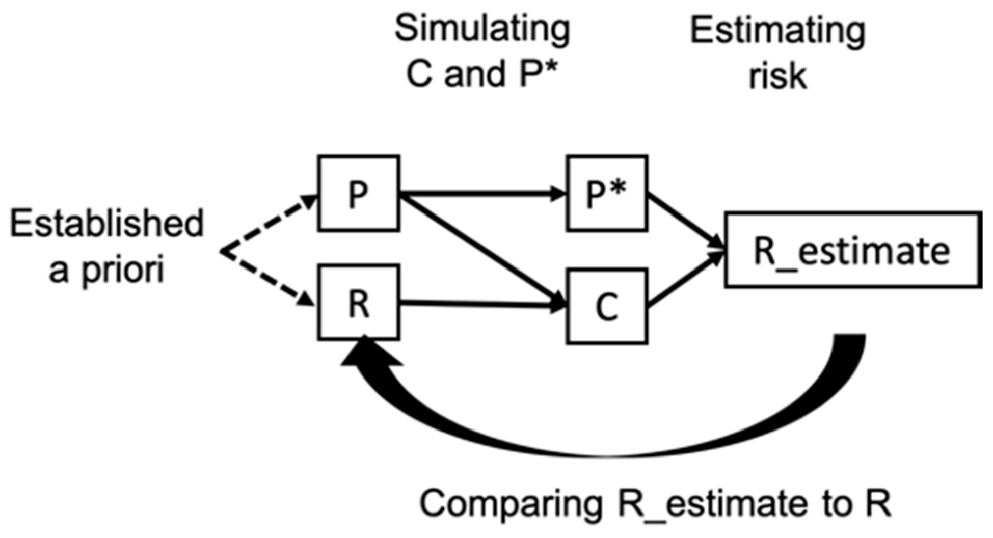
2.3. Validating the Method via a Simulation Study

The GWRisk method is validated using a simulation approach. While the theoretical basis for using GWR for estimating was provided in the former sections, a more empirical test is described here. In real world applications, we often do not know the actual victimization risk being estimated, and, as such, it becomes difficult to directly evaluate the performance of the proposed methodology in these situations. Therefore, the alternative is to test the proposed method under a controlled simulated case study. In this research, two controlled studies were conducted, the first using only one reference population (and one victimization risk), and the second using two reference populations (each with a different victimization risk map). The following details are valid for both studies.

If a reference populations size$P$ and victimization risk $R$ are known, as well as their associated error factors ${\mathit{\epsilon }}_C$ and ${\mathit{\epsilon }}_P$(assumed Gaussian) and reporting rate f (assumed 100% for simplicity), then observed crime count $C$ and observed population size $P^{*}$ can be simulated respectively as:

$$C ~ \mathit{Binomial}\left(p=R,n=P\right)+\mathit{Normal}\left(\mathit{mean}=0,sd={\mathit{\epsilon }}_C\right)$$

(19)

$$P^{*}~ \mathit{Normal}\left(\mathit{mean}=P,sd={\mathit{\epsilon }}_P\right)$$

(20)

Then, having $C$ and $P^{*}$, the risk $R$ can be estimated using the GWRisk method (or others) and the estimate compared to its true known value (defined a priori). This way, the effectiveness of the GWRisk method can be assessed, as well as how it compares to other competing methods. Figure 1 illustrates the simulation framework.

In this research, the simulation procedure just described was executed for multiple different case studies. The simulation study was done both for a case with one reference population (e.g., number of burglaries for the crime and number of residences as the population) and for a case with two reference populations (e.g., number of burglaries for the crime, number of houses as one of the populations and number of apartments as the other); moreover, for each study, multiple different combinations of $R$ and $P$ were used. It is worth noting that, at least from the theoretical point of view described in the former subsection, GWRisk may be used for more than two references population, and cases with three or more populations were not tested here due to size constraints for the study.

To automate the generation of different maps for $R$ and $P$, a geostatistical function $F$ for generating random surfaces was employed. Briefly describing, the function generates a random set of points (each with a random scalar value) within an area and then interpolates it using a variogram model (i.e., kriging interpolation) that dictates how spatial autocorrelated the interpolated values should be (for more on variograms and kriging, see [42,43,44]). The specific variogram model used in this study was the Exponential, which is based on parameters such as range (i.e., distance within which spatial autocorrelation can be found), sill (i.e., variance between uncorrelated samples), and nugget (i.e., variance for samples at an infinitesimal distance):

$$R ~ F\left({\mathit{range}}_R,sil{l}_R,{\mathit{nugget}}_R\right)$$

(21)

$$P ~ F\left({\mathit{range}}_P,sil{l}_P,{\mathit{nugget}}_P\right)$$

(22)

An initial set of values for the surface parameters was used so that $R$ and $P$ emulate the patterns observed in the real-world Belo Horizonte case (described in the following section), and then these values were changed in increments, to test the sensitivity of the estimates. Different values for the error factor ${\mathit{\epsilon }}_C$ also where tested, while a ${\mathit{\epsilon }}_P$ of 1% (in relation to the value of $P$) was used for all cases, that being based on the error rate estimated for the Brazilian Census 2010 (grounding the errors to a magnitude observed in real-world cases, although different errors magnitudes could be justifiable and tested in the future). The effectiveness of the GWRisk method was compared to that of using naïve standardization or local Empirical Bayesian Estimators, with the fitness metric being the R-square obtained when fitting the estimated risk to the true risk (i.e., the “ground truth”) under an Ordinary Least-Squares Method (other fitness metrics such as correlation could also be used but were not considered in this study due to size constraints). Notice that, although a reporting rate of $f=100\%,$ the same type of study would be possible with other values of $f$ since GWRisk estimates $fR$ (the reported victimization risk) not $R$ (the total victimization risk). Finally, it is important to notice that, while a Gaussian kernel was used in all the different iterations, the bandwidth was re-estimated for the new dataset using the cross-validation method. In addition, notice that geostatistical function $F$ was generated not from a Gaussian variogram but using the Exponential model and therefore the effectiveness of the GWRisk method is not being inflated by choosing the very same kernel (which would not be known for sure in a real-world, non-simulated application).

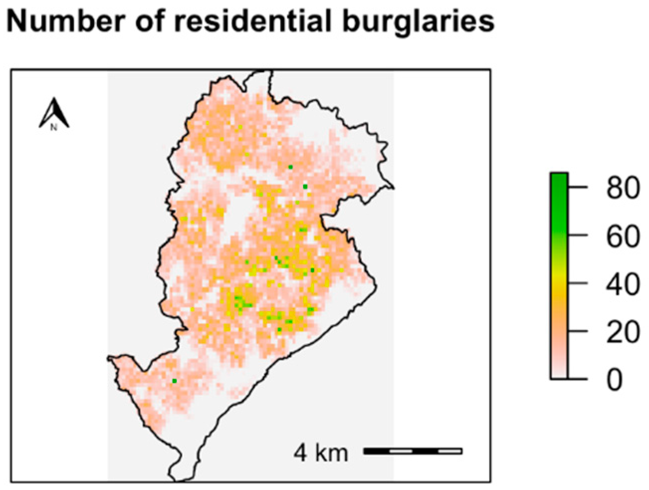
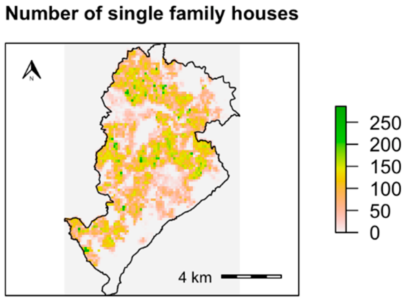
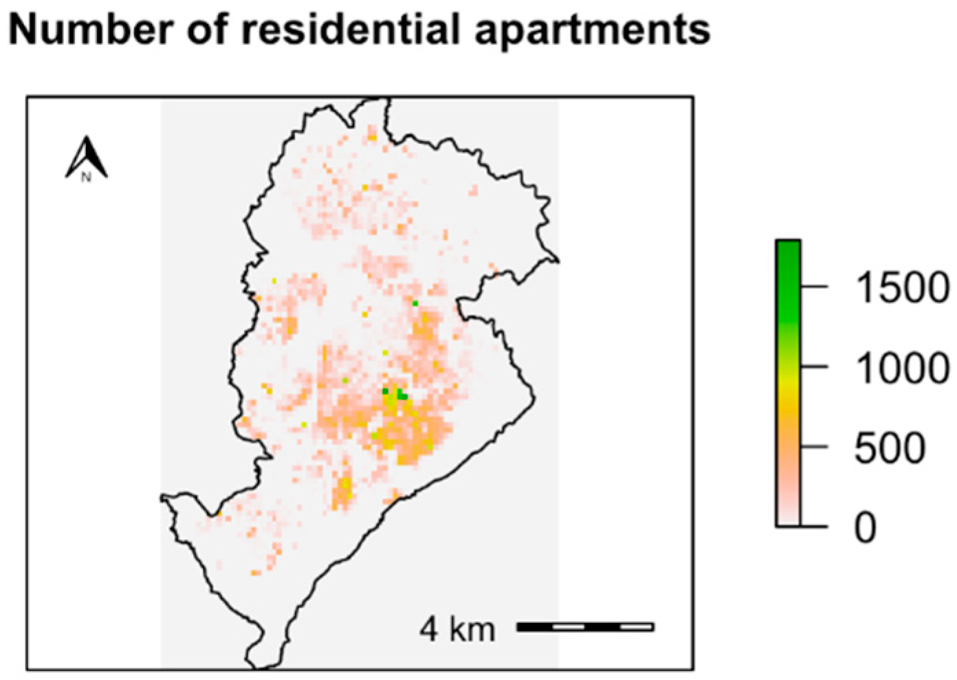
2.4. Application: Residential Burglaries in the City of Belo Horizonte, Brazil

To illustrate its use, the GWRisk method was applied to a real-world case, with the estimated risk being compared to that yielded by the naïve standardization procedure and using local Empirical Bayesian Estimators. Although naïve standardization and Empirical Bayesian Estimators are not the only other methods for estimating risk (as discussed in the Literature Review), these are some of the most common techniques used in crime mapping. Comparison between the GWRisk method and other approaches may be explored in future work.

The study case selected was that of residential burglaries in the city of Belo Horizonte, Brazil, for the period of 2008 to 2014. Risk of residential burglary is estimated for two reference populations: single-family houses and residential apartments. Data used in this part consist of geocoded point data for each individual residential burglary (44,560 points in total), as well as for each individual single-family house (206,281 points) and residential apartment (278,160 points). Burglary data originate from police records (Boletins de ocorrência da Polícia Militar de Minas Gerais), while residential data originate from real-estate tax register from the city of Belo Horizonte (IPTU). These point sets were then aggregated using a regular lattice with 100 rows and 76 columns, each areal unit being approximately a square of 278.75 m per side. The dimensions for the grid were determined by the method described in Ramos et al. [45], with this granularity providing a balance of robustness to error and internal uniformity to the crime. Figure 2, Figure 3 and Figure 4 show the maps for burglaries, houses, and apartments, respectively. Having these grids for crime counts and reference populations, the risks can be estimated through the GWRisk method or others.

3. Results

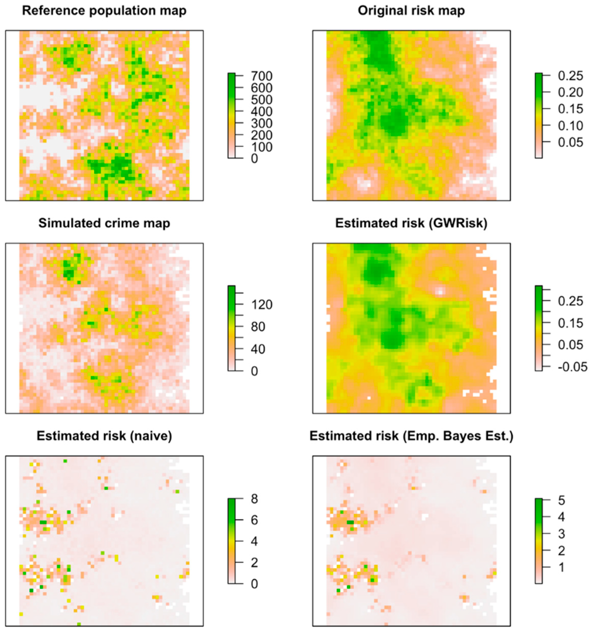
3.1. Results for the Validation Study

The simulation study shows that, on average, the GWRisk method performs better than the competing approaches tested. The following details the results for the validation study, first for the case with one reference population, then for the case with two reference populations.

3.1.1. Simulation Study with One Reference Population

Table 1. Summary of simulation study with one population, showing the mean values of the fitness scores for each method, as well as their standard deviations and coefficient of variations.

Fit for Estimated R	Mean	Std. Dev.	Coef. Var.
Fit (naïve)	0.16	0.08	52%
Fit (GWR)	0.61	0.08	14%
Fit (Bayes)	0.42	0.16	39%

summarizes the results for the simulation study with one reference population, showing the mean, standard deviations, and coefficient of variation of the fitness scores obtained. The list of parameters used in the simulation and their specific fitness scores is shown in Appendix B (

Table A1. Results of the simulation study with one population, showing the fitness scores for estimated risk calculated using three different methods, and using different parameters for generating maps of true risk R and reference population P. The unit for the range parameters is in number of map cells, while the units for sill and nugget correspond to the square of the unit for risk (i.e., the unit for its variance: crimes²/targets²). Bold was used to highlighted the parameters that area varying from row to row.

Parameter					Fit for Estimated R
rangeR	rangeP	sillP	nuggetP	${\mathbf{\epsilon }}_{\mathbf{C}}$	Fit (naïve)	Fit (GWRisk)	Fit (Bayes)
50	7	16,500	1250	15%	0.17	0.66	0.46
50	7	16,500	2500	15%	0.11	0.65	0.37
50	7	16,500	5000	15%	0.13	0.71	0.43
50	7	16,500	10,000	15%	0.17	0.71	0.48
75	7	16,500	1250	15%	0.13	0.65	0.39
25	7	16,500	1250	15%	0.17	0.68	0.46
10	7	16,500	1250	15%	0.17	0.57	0.50
5	7	16,500	1250	15%	0.23	0.39	0.50
50	3.5	16,500	1250	15%	0.12	0.73	0.42
50	14	16,500	1250	15%	0.16	0.60	0.44
50	28	16,500	1250	15%	0.26	0.59	0.55
50	56	16,500	1250	15%	0.40	0.57	0.60
50	7	10,000	1250	15%	0.18	0.66	0.52
50	7	20,000	1250	15%	0.14	0.69	0.44
50	7	40,000	1250	15%	0.12	0.71	0.34
50	7	80,000	1250	15%	0.09	0.68	0.28
50	7	16,500	1250	5%	0.32	0.68	0.76
50	7	16,500	1250	25%	0.08	0.63	0.20
50	7	16,500	1250	50%	0.03	0.65	0.06
50	7	16,500	1250	100%	0.01	0.54	0.02

). Notice how the GWRisk method not only has the greatest mean fitness score, but also has the lowest coefficient of variation. This coefficient of variation is also significantly smaller than the coefficient of variation for the parameters tested. Therefore, it can be concluded that, in this simulated experiment, not only is the risk estimated via the GWRisk method significantly better than the other options, but it is also more robust to parameter variations than the other methods.

Finally, Figure 5 illustrates a set of simulated maps for true victimizations risk, reference population and crime counts, and the corresponding estimated victimization risk using each method (naïve, GWRisk, and Empirical Bayesian Estimator methods). The figures exemplify how naïve standardization can lead to sharp peaks in some of the estimated values, peaks that are also observed using the Empirical Bayesian Estimator method, but eliminated when using the GWRisk method.

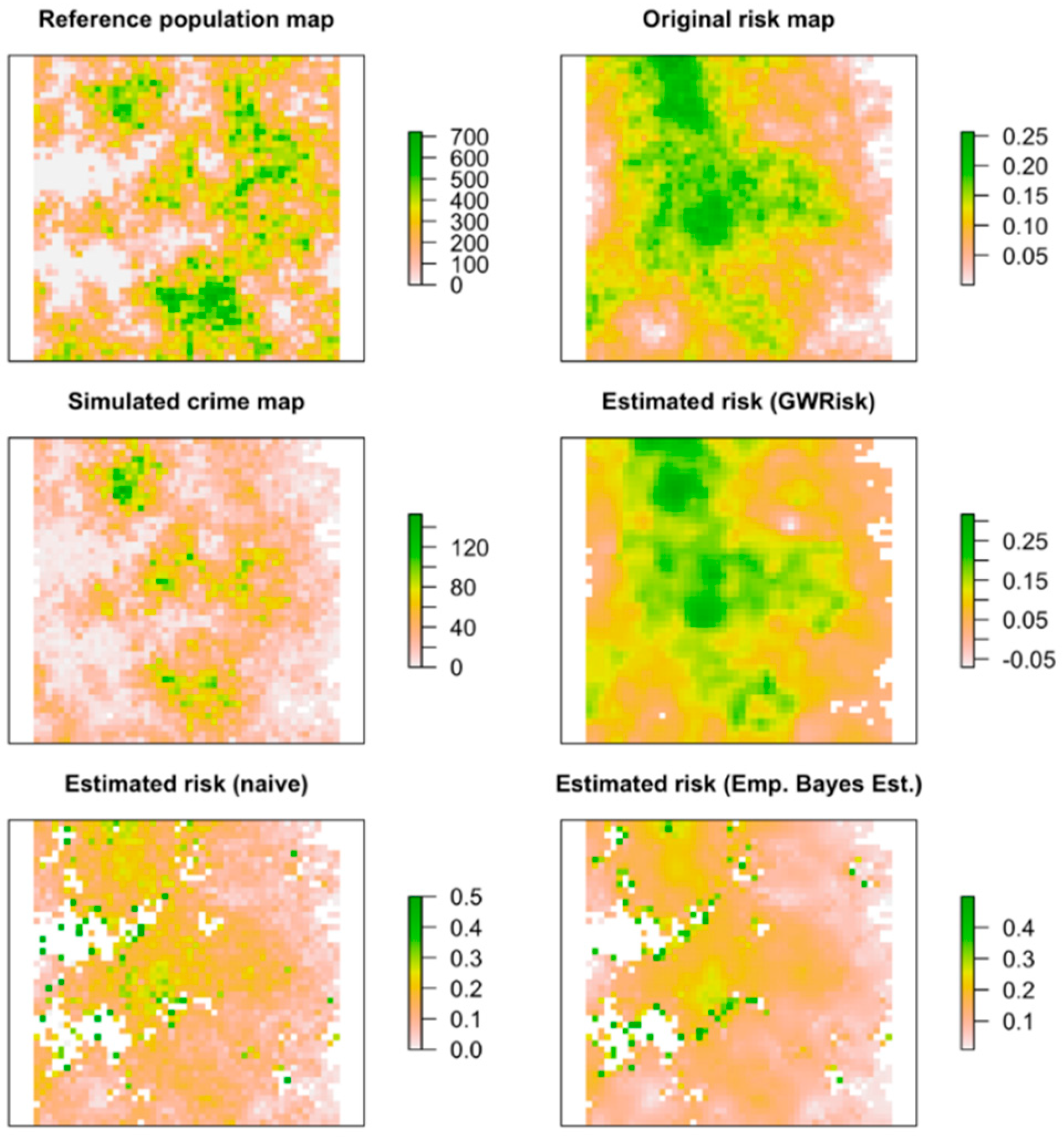
3.1.2. Simulation Study with Two Reference Population

The summary of the results for the simulation study with two reference populations is shown in

Table 2. Summary of the simulation study with two populations, showing the mean values of the fitness scores for each method, as well as their standard deviations and coefficient of variations.

	Mean	Std. Dev.	Coef. Var
Fit for estimated R1
Fit (naïve)	0.01	0.02	147%
Fit (GWR)	0.67	0.07	11%
Fit (Bayes)	0.02	0.03	148%
Fit for estimated R2
Fit (naïve)	0.01	0.00	47%
Fit (GWR)	0.28	0.08	29%
Fit (Bayes)	0.01	0.01	48%

. Tables with the individual values tested are included in the Supplementary Materials (Tables S1 and S2) due to formatting and space constraints reasons. Notice that, as in the study with one reference population, the GWRisk method not only provides a better mean fit, but that fit is more robust to variations in the parameter values (i.e., smallest coefficient of variation among the three methods tested).

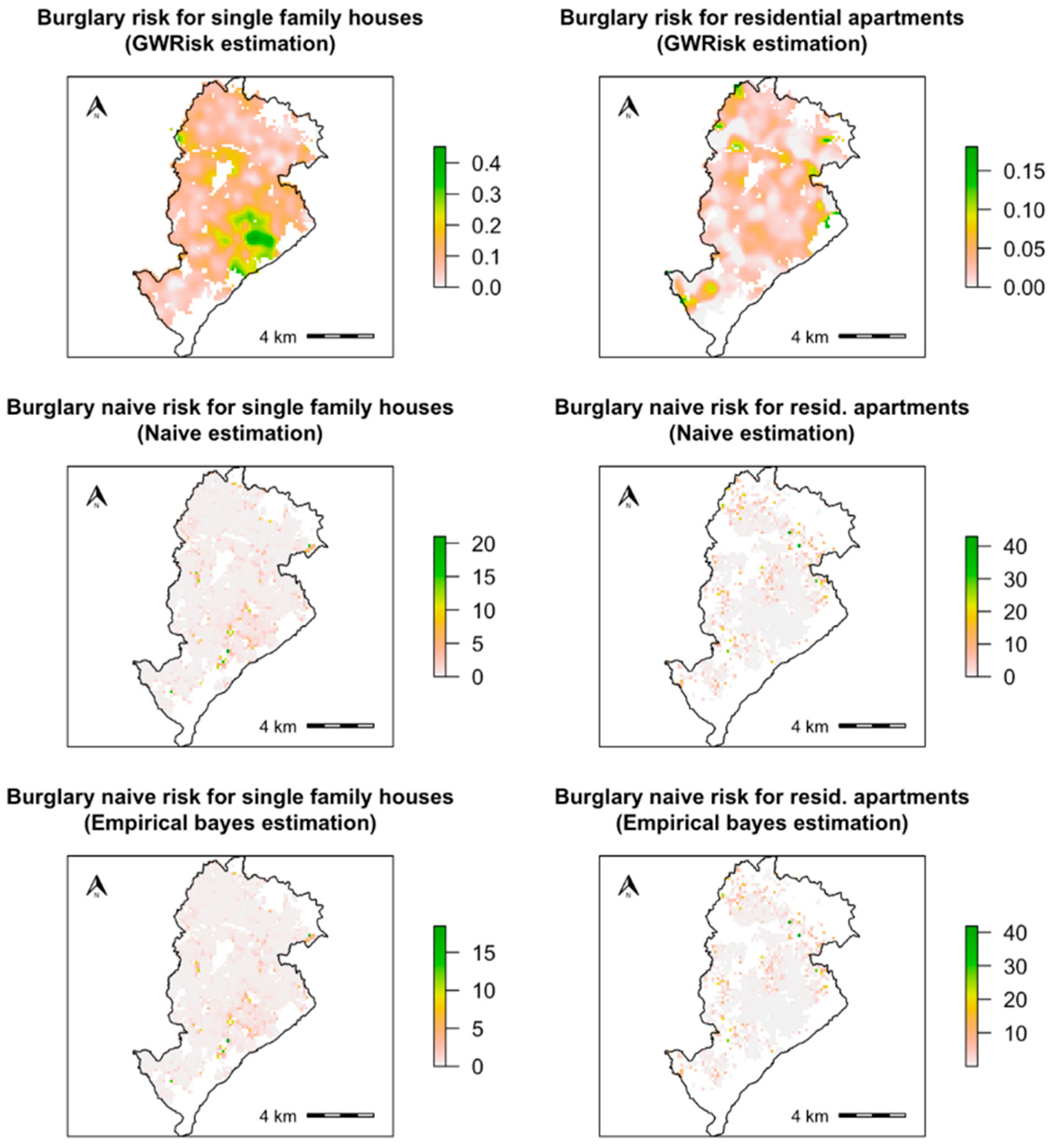
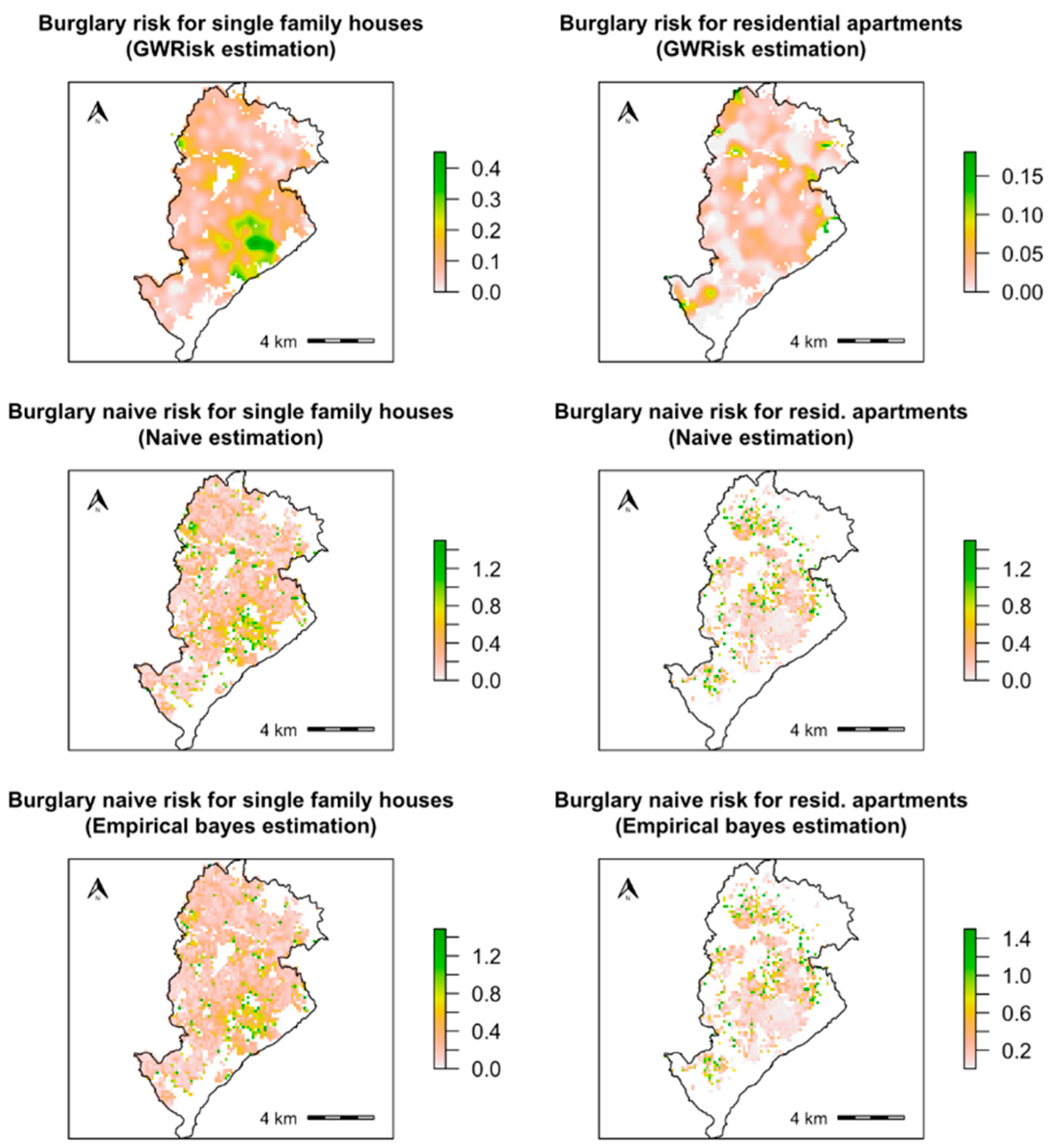
3.2. Results for the Application Study

The GWRisk method was used to estimate risk of burglary in the city of Belo Horizonte, Brazil. The risks estimated using the naïve method and the Empirical Bayesian Estimator method were also compared. The estimated risks using each of the three methods are shown in Figure 6. Notice how risk estimated with the naïve method and the Empirical Bayesian Estimator method feature multiple peaks, including areas with burglary risk as high as 25 burglaries per single-family house or 40 burglaries per residential apartment. These peaks are probably spurious, since these are more present in areas with small reference populations. On the other hand, the risk maps estimated with the GWRisk method do not feature these (probably spurious) peak, yielding smoother and easier to interpret maps.

4. Discussion

Standardized crime rates are useful for crime analysis, providing an estimate of victimization risk, but also involve multiple challenges. In this paper, these issues were consolidated into a mathematical framework, and a new method for tackling these problems was proposed. The proposed method, named GWRisk, uses Geographically Weighted Regression to estimate victimization risk by fitting a GWR model to explain crime counts varying as a function of a set of reference population sizes. In this approach, the fitted geographically varying coefficients associated with the reference populations can be interpreted as an estimate of the victimization risk. A controlled simulation study was conducted to compare the performance of the GWRisk method with the other two methods, i.e., the naïve standardization method and the local Empirical Bayesian Estimator method. The results of the simulation study showed that, for most cases tested, the GWRisk method performed best. Finally, an application of the GWRisk method to a real-world dataset was shown, estimating residential burglary risks for the city of Belo Horizonte, Brazil. The use of GWRisk provided smoother risk maps, contrary to the maps generated by the other two methods, which featured a series of peaks of risk (generally at locations with small population counts, and, thus, probably spurious). It is worth noting that, although the validation and application studies both used grids of square cells (rasters), the theoretical framework of the GWRisk does not assume this type of spatial unit, and other types of areal unit could be used (e.g., census tracts) or even units that are spatial but not areal such as street segments. The only assumption is that crimes and reference populations can be attributed to specific spatial units, and that victimization risk is spatially autocorrelated. The use of GWRisk on these other types of spatial unit may be explored in future research.

The GWRisk method has some limitations. For one, the risk estimation will still be affected by underreporting, and the estimated rate should be interpreted as the likelihood of an individual being a victim of a crime and reporting it. Nevertheless, this issue of underreporting is not exclusive to the method proposed here, and it can be partially mitigated if the average rate of reporting is known. Similarly, although GWRisk can auxiliate in determining adequate reference populations through regression diagnostics, it does not eliminate the issue completely. This is particularly important in the case of street crimes such as robbery, in which an adequate reference population (e.g., pedestrians) may be difficult to estimate. There are, however, methods estimating them [12,13,14,15,16], and the effectiveness for this type of crime could be investigated in future work. Another limitation is that the method requires spatial data, as well as a sufficiently large number of samples so that the geographically weighted regression can be performed. Standardization of crime rates is not necessarily conducted with spatial analysis in mind, and the location of the crimes might not be available in some situations; for some types of crime, their location may not even be very tangible (e.g., money laundering, fraud, cybercrimes). However, the GWRisk method was not designed with this application in mind; instead, it is most apt as a tool for mapping the risk of burglaries, robberies, thefts, and other spatially explicit crimes. In addition, the crime distribution that is being mapped may not conform to the statistical assumptions of the GWRisk method, impacting the accuracy of the estimated risk if that mismatch is severe. Variations of GWR may be a solution to this issue, such as binomial or Poisson implementations of GWR if the errors are not normally distribution, or MGWR to allow multiple bandwidths. This is particularly relevant in that crime counts are often expected to follow a Poisson (possibly zero-inflated) or some other non-Normal distribution, although, in this study, the standard GWR version worked well in practice. Finally, the validation study via simulation can be extended by including surfaces generated with different variogram models (e.g., Spherical, Gaussian), utilizing different criteria to select a kernel and bandwidth for GWRisk, and adding new alternative standardization methods for comparison; these extensions should provide more detail on the performance of GWRisk against other methods, and may be explored in future work. In addition, a systematic comparison between using one, two, or more reference populations when analyzing the same crime distribution (and how to identify the most adequate set of reference populations) could be explored, as well as the application of the GWRisk These variations will be examined in future work. Despite these limitations, GWRisk features as a valuable and robust approach for mapping victimization risk, circumventing instability problems present in other existing methods.

References

1. Biderman, A.D.; Reiss, A.J., Jr. On exploring the “dark figure" of crime. Ann. Am. Acad. Political. Soc. Sci. 1967, 374, 1–15. [Google Scholar] [CrossRef] [Green Version]
2. Radzinowicz, L.; King, J.F. The Growth of Crime: The International Experience; Basic Books: New York, NY, USA, 1977; pp. 3–9. [Google Scholar]
3. Payne, J.L.; Hutton, F. Mapping Common Crime. In The Palgrave Handbook of Australian and New Zealand Criminology, Crime and Justice; Palgrave Macmillan: Cham, Switzerland, 2017; pp. 113–129. [Google Scholar] [CrossRef]
4. Langton, L.; Planty, M.; Lynch, J.P. Second major redesign of the national crime victimization survey (ncvs). Criminol. Pub. Pol’y 2017, 16, 1049. [Google Scholar] [CrossRef]
5. Williams, D.; Edwards, S.; Giambo, P.; Kena, G. Cost Effective Mail Survey Design. In Proceedings of the Federal Committee on Statistical Methodology Research and Policy Conference, Washington, DC, USA, 1–3 December 2018. [Google Scholar]
6. Ratcliffe, J. Crime mapping: Spatial and temporal challenges. In Handbook of Quantitative Criminology; Springer: New York, NY, USA, 2010; pp. 5–24. [Google Scholar] [CrossRef]
7. Boggs, S.L. Urban crime patterns. Am. Sociol. Rev. 1965, 899–908. [Google Scholar] [CrossRef]
8. Solymosi, R.; Ashby, M.; Cohen, T.; Sidebottom, A. Alternative denominators in transport crime rates. SocArXiv 2017. [Google Scholar] [CrossRef]
9. Rengert, G.F. Burglary in Philadelphia: A critique of an opportunity structure model. In Environmental Criminology; Brantingham, P.J., Brantingham, P.L., Eds.; Sage: Beverly Hills, CA, USA, 1981; pp. 189–201. [Google Scholar]
10. Stipak, B. Alternatives to population-based crime rates. Int. J. Comp. Appl. Crim. Justice 1988, 12, 247–260. [Google Scholar] [CrossRef]
11. Pettiway, L.E. Measures of opportunity and the calculation of the arson rate: The connection between operationalization and association. J. Quant. Criminol. 1985, 1, 241–268. [Google Scholar] [CrossRef]
12. Kounadi, O.; Ristea, A.; Leitner, M.; Langford, C. Population at risk: Using areal interpolation and Twitter messages to create population models for burglaries and robberies. Cartogr. Geogr. Inf. Sci. 2018, 45, 205–220. [Google Scholar] [CrossRef]
13. Malleson, N.; Andresen, M.A. The impact of using social media data in crime rate calculations: Shifting hot spots and changing spatial patterns. Cartogr. Geogr. Inf. Sci. 2015, 42, 112–121. [Google Scholar] [CrossRef]
14. Andresen, M.A.; Jenion, G.W.; Reid, A.A. An evaluation of ambient population estimates for use in crime analysis. Crime Mapp. J. Res. Pract. 2012, 4, 7–30. [Google Scholar]
15. Chainey, S.; Desyllas, J. Modelling pedestrian movement to measure on-street crime risk. In Movement-Aware Applications for Sustainable Mobility: Technologies and Approaches; Wachowicz, M., Ed.; IGI Global: Hershey, PA, USA, 2010; pp. 243–263. [Google Scholar] [CrossRef]
16. Andresen, M.A. Crime measures and the spatial analysis of criminal activity. Br. J. Criminol. 2006, 46, 258–285. [Google Scholar] [CrossRef]
17. Eck, J.E.; Weisburd, D.L. Crime places in crime theory. In Crime and Place: Crime Prevention Studies; Hebrew University of Jerusalem Legal Research Paper: Jerusalem, Israel, 2015; Volume 4, pp. 1–33. Available online: https://ssrn.com/abstract=2629856 (accessed on 15 May 2021).
18. Weisburd, D.; Groff, E.R.; Yang, S.M. The Criminology of Place: Street Segments and Our Understanding of the Crime Problem; Oxford University Press: Oxford, UK, 2012. [Google Scholar]
19. Sherman, L.W.; Gartin, P.R.; Buerger, M.E. Hot spots of predatory crime: Routine activities and the criminology of place. Criminology 1989, 27, 27–56. [Google Scholar] [CrossRef]
20. Kafadar, K. Smoothing geographical data, particularly rates of disease. Stat. Med. 1996, 15, 2539–2560. [Google Scholar] [CrossRef]
21. Anselin, L.; Kim, Y.W.; Syabri, I. Web-based analytical tools for the exploration of spatial data. J. Geogr. Syst. 2014, 6, 197–218. [Google Scholar] [CrossRef]
22. Beato Filho, C.C.; Assunção, R.M.; Silva, B.F.A.D.; Marinho, F.C.; Reis, I.A.; Almeida, M.C.D.M. Conglomerados de homicídios e o tráfico de drogas em Belo Horizonte, Minas Gerais, Brasil, de 1995 a 1999. Cadernos de Saúde Pública 2001, 17, 1163–1171. [Google Scholar] [CrossRef]
23. Santos, A.E.; Rodrigues, A.L.; Lopes, D.L. Aplicações de Estimadores Bayesianos Empíricos para Análise Espacial de Taxas de Mortalidade. In Proceedings of the Simpósio Brasilerio de Geoinformática, 7 (GeoInfo), Campos do Jordão, Brazil, 20–23 November 2005; pp. 300–309. [Google Scholar]
24. Liu, H.; Zhu, X. Exploring the influence of neighborhood characteristics on burglary risks: A Bayesian random effects modeling approach. ISPRS Int. J. Geo-Inf. 2016, 5, 102. [Google Scholar] [CrossRef] [Green Version]
25. Zhu, L.; Gorman, D.M.; Horel, S. Hierarchical Bayesian spatial models for alcohol availability, drug" hot spots" and violent crime. Int. J. Health Geogr. 2006, 5, 54. [Google Scholar] [CrossRef] [Green Version]
26. Song, C.; He, Y.; Bo, Y.; Wang, J.; Ren, Z.; Yang, H. Risk assessment and mapping of hand, foot, and mouth disease at the county level in mainland China using spatiotemporal zero-inflated Bayesian hierarchical models. Int. J. Environ. Res. Public Health 2018, 15, 1476. [Google Scholar] [CrossRef] [Green Version]
27. Lai, Y.S.; Zhou, X.N.; Pan, Z.H.; Utzinger, J.; Vounatsou, P. Risk mapping of clonorchiasis in the People’s Republic of China: A systematic review and Bayesian geostatistical analysis. PLoS Negl. Trop. Dis. 2017, 11. [Google Scholar] [CrossRef] [PubMed] [Green Version]
28. Tzala, E.; Best, N. Bayesian latent variable modelling of multivariate spatio-temporal variation in cancer mortality. Stat. Methods Med Res. 2008, 17, 97–118. [Google Scholar] [CrossRef]
29. Bailey, T.C.; Cordeiro, R.; Lourenço, R.W. Semiparametric modeling of the spatial distribution of occupational accident risk in the casual labor market, Piracicaba, Southeast Brazil. Risk Anal. Int. J. 2007, 27, 421–431. [Google Scholar] [CrossRef] [PubMed]
30. Kelsall, J.E.; Diggle, P.J. Spatial variation in risk of disease: A nonparametric binary regression approach. J. R. Stat. Soc. Ser. C 1998, 47, 559–573. [Google Scholar] [CrossRef]
31. Brunsdon, C.; Fotheringham, A.S.; Charlton, M.E. Geographically weighted regression: A method for exploring spatial nonstationarity. Geogr. Anal. 1996, 28, 281–298. [Google Scholar] [CrossRef]
32. Fotheringham, A.S.; Charlton, M.E.; Brunsdon, C. Geographically weighted regression: A natural evolution of the expansion method for spatial data analysis. Environ. Plan. A 1998, 30, 1905–1927. [Google Scholar] [CrossRef]
33. Bitter, C.; Mulligan, G.F.; Dall’erba, S. Incorporating spatial variation in housing attribute prices: A comparison of geographically weighted regression and the spatial expansion method. J. Geogr. Syst. 2007, 9, 7–27. [Google Scholar] [CrossRef] [Green Version]
34. Chang, L.F.; Lin, C.H.; Su, M.D. Application of geographic weighted regression to establish flood-damage functions reflecting spatial variation. Water SA 2008, 34, 209–216. [Google Scholar] [CrossRef] [Green Version]
35. Cardozo, O.D.; García-Palomares, J.C.; Gutiérrez, J. Application of geographically weighted regression to the direct forecasting of transit ridership at station-level. Appl. Geogr. 2012, 34, 548–558. [Google Scholar] [CrossRef]
36. Huang, B.; Wu, B.; Barry, M. Geographically and temporally weighted regression for modeling spatio-temporal variation in house prices. Int. J. Geogr. Inf. Sci. 2010, 24, 383–401. [Google Scholar] [CrossRef]
37. Fotheringham, A.S.; Yang, W.; Kang, W. Multiscale geographically weighted regression (MGWR). Ann. Am. Assoc. Geogr. 2017, 107, 1247–1265. [Google Scholar] [CrossRef]
38. Wu, C.; Ren, F.; Hu, W.; Du, Q. Multiscale geographically and temporally weighted regression: Exploring the spatiotemporal determinants of housing prices. Int. J. Geogr. Inf. Sci. 2019, 33, 489–511. [Google Scholar] [CrossRef]
39. Tobler, W.R. A computer movie simulating urban growth in the Detroit region. Econ. Geogr. 1970, 46, 234–240. [Google Scholar] [CrossRef]
40. Comber, A.; Brunsdon, C.; Charlton, M.; Dong, G.; Harris, R.; Lu, B.; Lü, Y.; Murakami, D.; Nakaya, T.; Wang, Y.; et al. The GWR route map: A guide to the informed application of Geographically Weighted Regression. arXiv 2020, arXiv:2004.06070. [Google Scholar]
41. Farber, S.; Páez, A. A systematic investigation of cross-validation in GWR model estimation: Empirical analysis and Monte Carlo simulations. J. Geogr. Syst. 2007, 9, 371–396. [Google Scholar] [CrossRef]
42. Chiles, J.P.; Delfiner, P. Geostatistics: Modeling Spatial Uncertainty; John Wiley & Sons: Hoboken, NJ, USA, 2009; Volume 487. [Google Scholar] [CrossRef]
43. Oliver, M.A.; Webster, R. Basic Steps in Geostatistics: The Variogram and Kriging; Springer International Publishing: New York, NY, USA, 2015. [Google Scholar] [CrossRef]
44. Schabenberger, O.; Gotway, C.A. Statistical Methods for Spatial Data Analysis; CRC Press: Boca Raton, FL, USA, 2017. [Google Scholar] [CrossRef]
45. Ramos, R.G.; Silva, B.F.; Clarke, K.C.; Prates, M. Too Fine to be Good? Issues of Granularity, Uniformity and Error in Spatial Crime Analysis. J. Quant. Criminol. 2020, 1–25. [Google Scholar] [CrossRef]
Figure 1. Simulation framework to validate the GWRisk method.
Ijgi 10 00364 g001
Figure 2. Map of residential burglaries in Belo Horizonte, Brazil, from 2008 to 2014. Grid used consists of uniform square cells of 278.5 m per side.
Ijgi 10 00364 g002
Figure 3. Map of single-family houses in Belo Horizonte, using real-estate tax records from 2010.
Ijgi 10 00364 g003
Figure 4. Map of apartments in Belo Horizonte, using real-estate tax records from 2010.
Ijgi 10 00364 g004
Figure 5. An example case showing maps for simulated reference population, (true) victimization risk and crime counts, as well as the estimated victimization risks using each of the three methods considered: GWRisk, naïve estimation, and the Empirical Bayes Estimator method. Parameters for this case are listed in Table A1 (Appendix B), 15th entry.
Ijgi 10 00364 g005
Figure 6. Estimated victimization risks of burglary for single-family houses and residential apartments, calculated using each of the three methods tested. See Figure A2 in Appendix C for naïve and Empirical Bayes maps with very high values removed.
Ijgi 10 00364 g006