Article

Seismic Vulnerability Assessment in Ranau, Sabah, Using Two Different Models

1
Malaysia-Japan International Institute of Technology (MJIIT), University Teknologi Malaysia, Jalan Sultan Yahya Petra, Kuala Lumpur 54100, Malaysia
2
Department of Survey and Mapping Malaysia (JUPEM), Jalan Sultan Yahya Petra, Kuala Lumpur 50578, Malaysia
3
Department of Restoration Ecology and Built Environment, Tokyo City University, 1-28-1 Tamazutsumi, Setagay-ku, Tokyo 158-8557, Japan
*
Author to whom correspondence should be addressed.
ISPRS Int. J. Geo-Inf. 2021, 10(5), 271; https://doi.org/10.3390/ijgi10050271
Submission received: 4 March 2021 / Revised: 19 April 2021 / Accepted: 21 April 2021 / Published: 23 April 2021

Abstract

:
Sabah is prone to seismic activities due to its location, being geographically located near the boundaries of three major active tectonic plates; the Eurasian, India-Australia, and Philippine-Pacific plates. The 6.0 Mw earthquake that occurred in Ranau, Sabah, on 15 June 2015 which caused 18 casualties, all of them climbers of Mount Kinabalu, raised many issues, primarily the requirements for seismic vulnerability assessment for this region. This study employed frequency ratio (FR)–index of entropy (IoE) and a combination of (FR-IoE) with an analytical hierarchy process (AHP) to map seismic vulnerability for Ranau, Sabah. The results showed that the success rate and prediction rate for the areas under the relative operating characteristic (ROC) curves were 0.853; 0.856 for the FR-IoE model and 0.863; 0.906 for (FR-IoE) AHP, respectively, with the highest performance achieved using the (FR-IoE) AHP model. The vulnerability maps produced were classified into five classes; very low, low, moderate, high, and very high seismic vulnerability. Seismic activities density ratio analysis performed on the final seismic vulnerability maps showed that high seismic activity density ratios were observed for high vulnerability zones with the values of 9.119 and 8.687 for FR-IoE and (FR-IoE) AHP models, respectively.

1. Introduction

The past seismo-tectonic studies of South-East Asia showed that Malaysia faces a certain level of risk from magnitude >5.0 earthquakes originating from the surrounding regions as well as from local seismic tremors [1]. Malaysia is considered as lying in a low seismic region; although located less than 300 km from the tectonically active Pacific Ring of Fire [2]. However, Malaysia is still exposed to earthquake risk as it is located near to the most two seismically active plate boundaries, the inter-plate boundary between the Indo-Australian and Eurasian Plates on the west and the inter-plate boundary between the Eurasian and Philippines Sea Plates on the east [3].
Although being considered as seismically stable with no current history of major seismic and volcanic activity, the East Malaysia region, particularly Sabah, is at risk of moderate magnitude earthquakes due to the fact of its proximity to an active tectonic zone; the Ring of Fire, with the earliest record earthquake in the country occurring in the state in 1976 in Lahad Datu at 5.3 magnitude [4]. An earthquake occurred in Ranau, Sabah, on 5 June 2015 at 6.0-moment magnitude scale (Mw) and VII Modified Mercalli Intensity (MMI) drawing huge attention from the government and relevant authorities on the study of seismic activities in Sabah [4,5] particularly on seismic vulnerability, hazard and risk assessment [6,7]. The 6.0 Mw earthquake also progressively developed into prolonged aftershocks in the form of ground shaking; poses a bigger threat to the community living within the seismic activity zone and triggering geological hazards such as mud-floods.
Evidence data from the Minerals and Geoscience Department (JMG) reported that Ranau has strong topographic relief and even moderate magnitude earthquakes would generate large-scale mass movements of land; landslides and mud-floods [8]. These issues created urgent needs for the general population especially for the people living in the affected zone and required immediate solutions towards disaster recovery and preparedness; prompting research-based outputs [4].
Based on past seismic activities in Sabah and its location near the active plate boundaries, a seismic risk assessment map of Sabah particularly for the Ranau district at different probability levels is deemed required. A risk map requires combination analysis on the seismic vulnerability and hazard of the area of interest. However, only seismic vulnerability of the study area would be the highlight of this study using methodologies adopted from landslide susceptibility analysis following studies from [9,10,11,12,13], just to name a few.
Vulnerability expresses the tendency of elements at risk to sustain a certain damage level in a suitably defined damage scale [14]. Seismic vulnerability in this study was expressed in terms of an index to analyze conditions controlled by physical and environmental factors, which increase the susceptibility of a community in the study area to the impact of seismic hazards [15]. Several methods for the seismic vulnerability mapping have been developed, proposed and adopted in recent years including Geographic Information System (GIS)-based multicriteria decision analysis (MCDA) [16], simple additive weighting (SAW) [16], analytical hierarchy process (AHP) [17,18,19], analytical network process (ANP) [17,20], logistic regression (LR) [17,21,22], support vector machine (SVM) [21], artificial neural network (ANN) [23], ANP-ANN [24], random forest (RF) along with decision tree (DT) and frequency ratio (FR) by [25] and step-wise weight assessment ratio analysis (SWARA) [26]. Reference [17] also combined various models to produce four hybrid models of; (1) fuzzy logic (fuzzy) with logistic regression (LR) (abbreviated as fuzzy-LR), (2) fuzzy with analytical network process (ANP) and AHP (abbreviated as A-fuzzy), (3) ANP and AHP with ordered weight averaging (OWA) (abbreviated as (A-OWA) and (4) OWA-LR. The approaches and methodologies applied had been proven to be capable of assessing seismic vulnerability in their respective areas of interest.
In this study, two models namely Index of Entropy (IoE) by incorporating the frequency ratio (FR) model and a combination of (FR-IoE)- AHP were used to produce seismic vulnerability maps along with GIS technology. Two main indicators; environmental and physical indicators consisting of nine conditional factors and thirty-seven classes were applied. The performances of the final seismic vulnerability maps were accessed based on the area under the curve (AUC) values of the receiver operating characteristics (ROC) curve. In addition, the percentage distribution of past seismic activities and the area covered by each of the five vulnerability classes; very low, low, moderate, high, and very high were validated through past seismic activities’ density analysis to compare the consistency and correlation between the two models.
There are two noteworthy aspects in this study. One, is that although the combination of FR-IoE model had been extensively used for other natural hazards-related research such as [27,28,29], the combination of the FR-IoE model was either rarely or never applied for seismic vulnerability assessment particularly in the study area. Thus, this study intended to investigate whether the same method could be applied to a seismic vulnerability study. The main design was that past seismic activities’ epicenters were used in modeling the seismic vulnerability map which was similar to the ways landslide inventory data are used for landslide susceptibility mapping and flood inventory data are used for flood susceptibility or prone areas mapping. The second significant aspect of this study is the experimentation of the hybrid (FR-IoE) AHP model in a disaster-related study. This study tried to improve the ‘vague’ decision-making process of assigning weightage in AHP by implementing FR-IoE result in the AHP methodological structure. Interestingly, this study found that the AUC values obtained by the (FR-IoE) AHP model for both training and testing regimes were higher than the values obtained from the FR-IoE model.

2. Materials and Methods
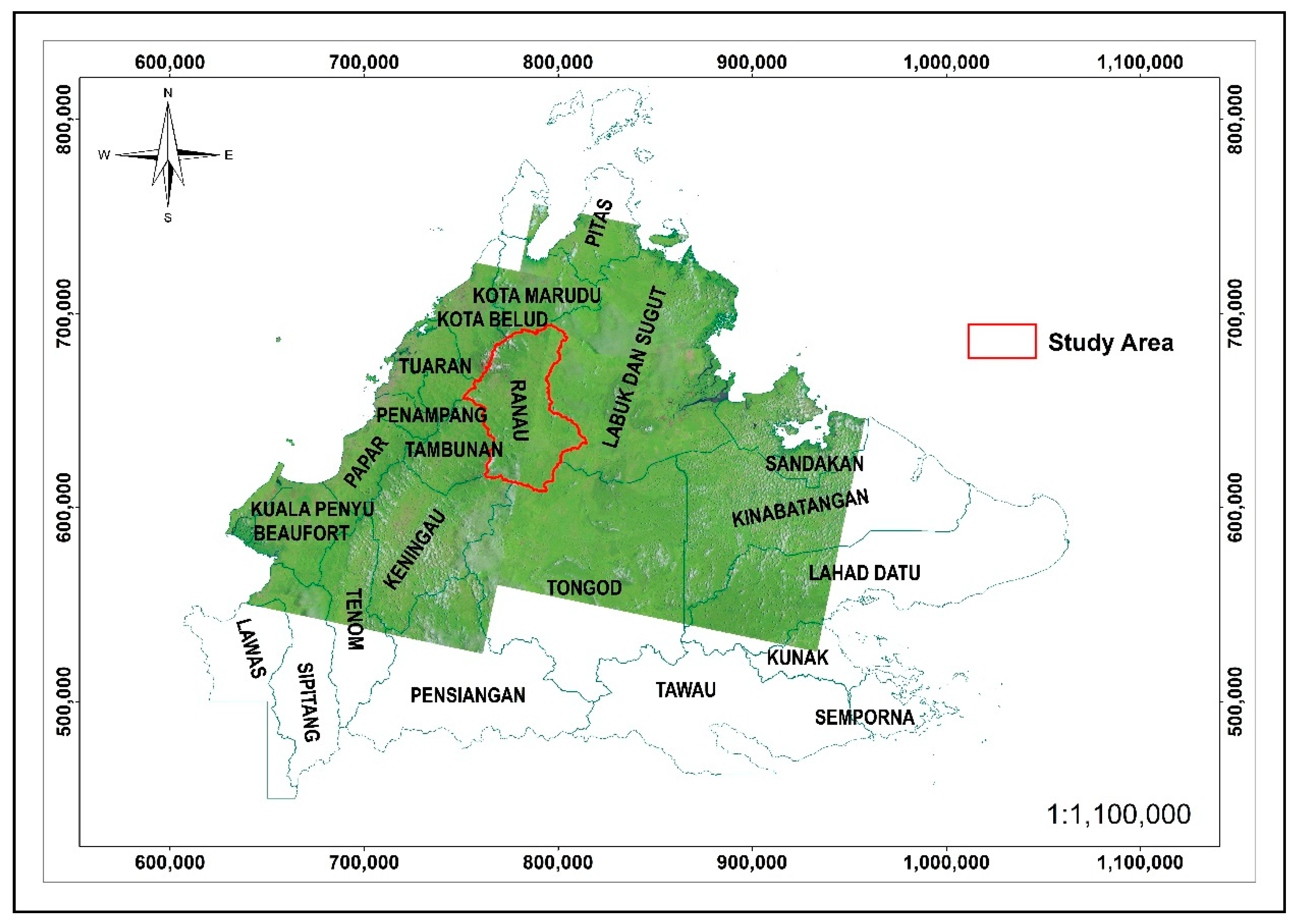
2.1. Study Area

Ranau district as shown in Figure 1 is one of the administrative districts in Sabah, geographically located between 5°30’ N to 6°25’ N and 116°30’ E to 117°5’ E, covering an area of 3555.51 km2 (1372.79 square miles) [30]. The district is surrounded by Kota Marudu to the north, Kota Belud to the northeast, Tuaran to the west, Tambunan to the southwest, Keningau to the south, Tongod to the southeast, and Beluran to the east [31]. It is characterized by the Crocker Range in its northern part and the Pinousok summit which runs in a southwesterly direction. The Ranau plain and Trus Madi Range cover its eastern side and the southern part is bounded by the Labuk highlands [30]. The geography is predominantly attributed to its mountainous landforms most notably; Mount Kinabalu with a valley plain. Based on the 2010 census by the Department of Statistics Malaysia, the population of the district was 94,092 [31].
The existence of active faults in Sabah is proved by geomorphological features, such as triangular facets, stream offsets, mud volcanoes, and hot springs [32]. The 5 June 2015 6.0 Mw earthquake which struck Ranau reinforced active faults in Sabah [33]. This earthquake suggests that the faulty lines around the tectonic landform in the region are active and, in the future, the seismically active plate is capable of generating an even greater earthquake in terms of its magnitude or intensity scale.

2.2. Conditional Factors

The first step to producing the seismic vulnerability assessment map is the identification of the factors that are the main attributes that concern the environmental, social, and economic settings of the region and the available infrastructure [10,34]. In this study, a total of nine conditional factors or parameters with 37 classes from two main indicators were considered. Examples of physical indicators are street pattern, building density, building alignment, open space density, land cover and other built-environment related factors [35,36] and examples of environmental factors include slope, geological features, aspect, fault and other natural-related features [24]. According to [37], in GIS-based studies, the selected factors should be operational, complete, non-uniform, measurable, and non-redundant. Most of the datasets used were extracted from the Department of Survey and Mapping Malaysia (JUPEM) MY611T 1:25,000 scale topographic map through spatial analysis which included distance from buildings, altitude, distance from rivers, distance from streams, distance from roads, distance from tracks and slope angle. Distance from faulty lines data were extracted from Department of Mineral and Geoscience Malaysia (JMG) fault data. Lithology data were obtained from United States Geological Survey (USGS) World Geologic Maps.
ArcGIS software was used to process the required conditional factors which include generating the weightage for each factor in ArcMap Attribute Table and rasterization of the parameters involved to compute vulnerability index map using ‘Raster Calculator’. Past earthquake data were obtained from USGS: Earthquake Hazard Program website which stored only major earthquake event data and from Malaysia Meteorological Department (MetMalaysia). The total past earthquake data obtained from both USGS and MetMalaysia are 130 points (the earthquake epicenters) but only 84 points fell within Ranau area. From these 84 points; 60 points (71.43%) were used to compute the seismic vulnerability map. The other 24 points (28.57%) were used to validate the two models using statistical computation of ROC. The past earthquake data range from the year 1991 with the latest data from the year 2019 as shown in Figure 2a.

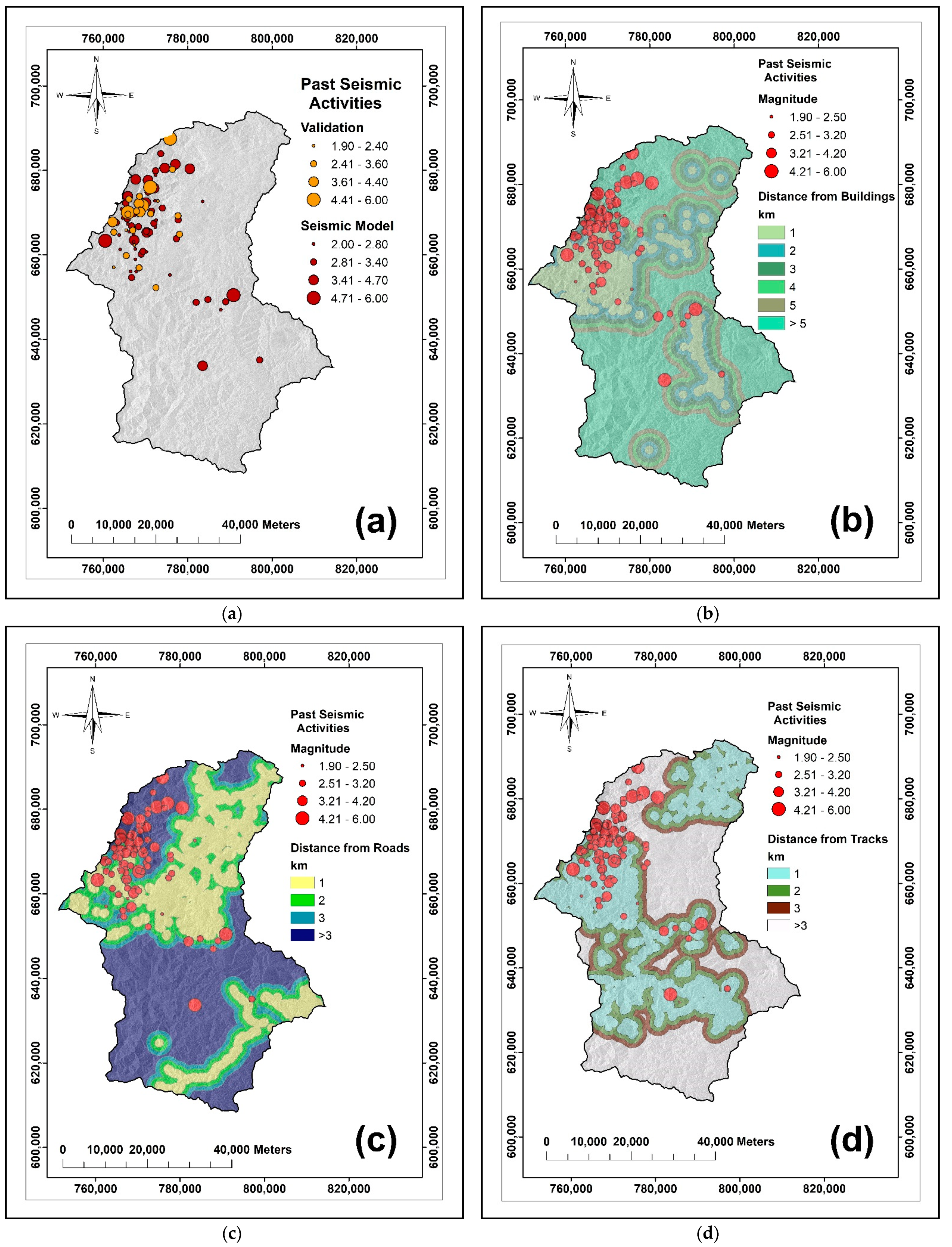
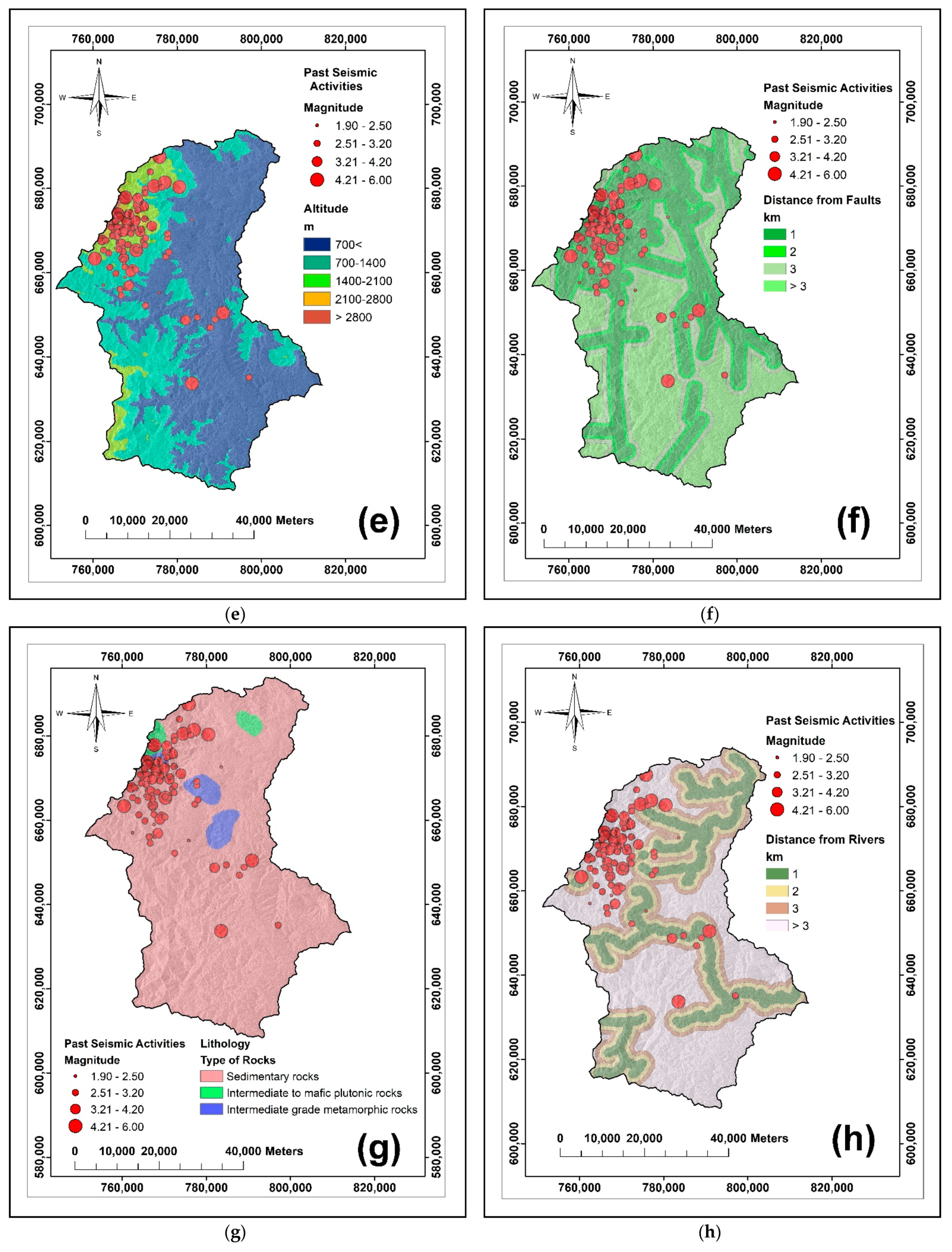
2.2.1. Physical Indicators

Distance from buildings (Figure 2b). Building data play an important role in seismic vulnerability assessment as the distance or closeness of these buildings from location(s) with significant tectonic activity determining the risk of people associated with these buildings to exposure to injury and death during an earthquake [38].
Distance from roads and distance from tracks (Figure 2c,d). Road features refer to a paved route or major road whereby track refers to an unpaved road or muddy trail used by the population in Ranau. Transportation networks are important in escaping dangerous situations and facilitating the relief and assistance of the injured require roads and streets for vehicles to pass [17]. Transportation networks also vulnerable to damages during an earthquake. An earthquake can cause fissures, sinkholes and cracks that cut roads and cause vehicles to plunge into sinkholes that suddenly appear before, during or after a main shock [39]. Instead of being a tool for emergency response, roads especially paved ones can be lethal to their users. Thus, it is important to identify which parts or location of the transportation networks in this study are within “highly vulnerable” areas to capture the impacts of extreme earthquakes in the future [40].

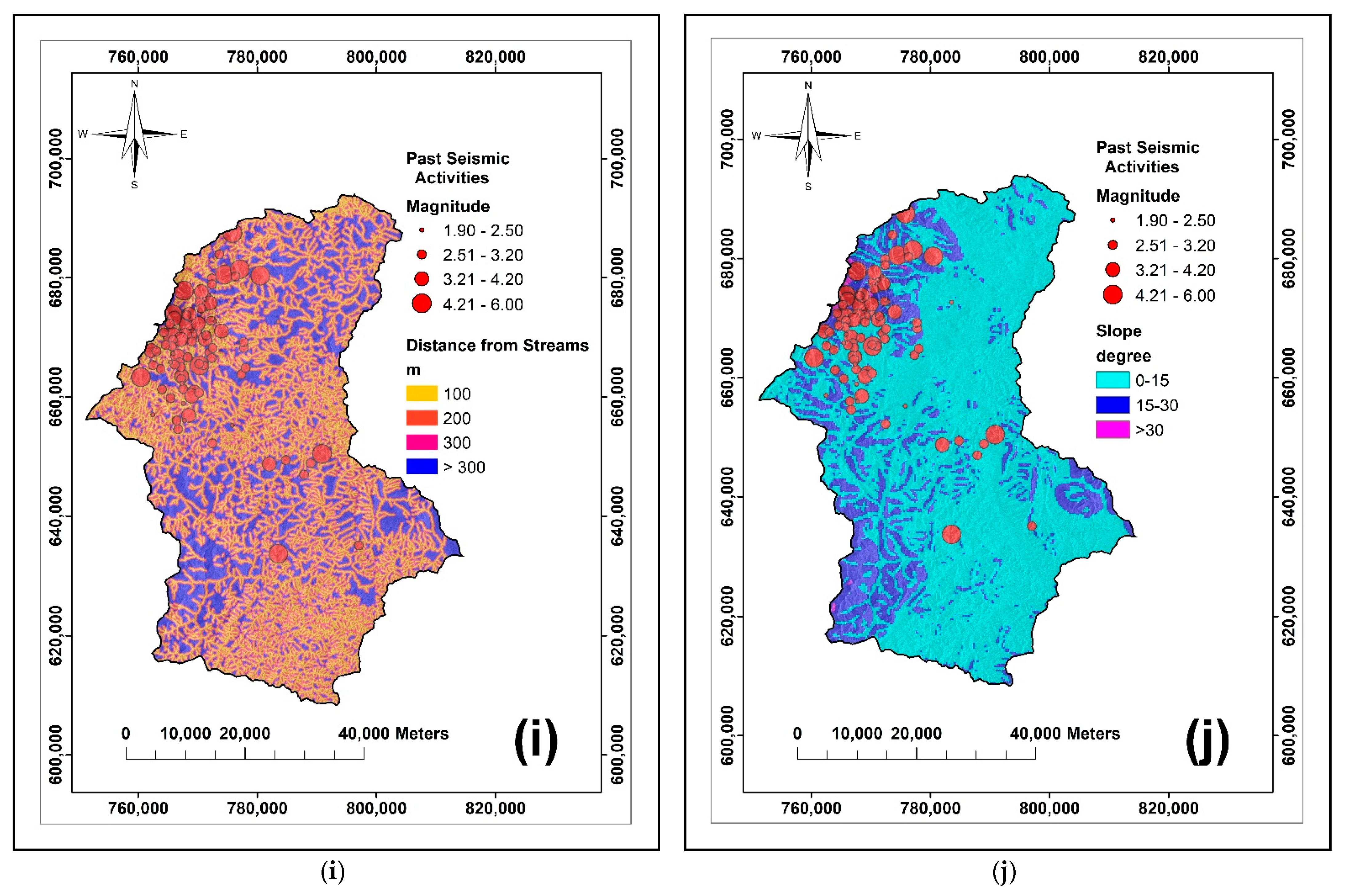
2.2.2. Environmental Indicators

Altitude (Figure 2e). The high and low elevations are deeply linked with the occurrence of landslides and mudslides [17,41] in many earthquake events [42,43,44,45].
Distance from fault lines (Figure 2f). According to [33], earthquakes in Sabah are generated by thrust faults, strike-slip faults and normal faults. In the 2015 Ranau earthquake, the Focal Mechanism Solution (FMS) carried by USGS showed that the fault plane that was produced by the main shock was caused by a normal fault. Fault data were important in vulnerability assessment as earthquakes occur on faults regardless of whether they are thrust-faults, strike-slip faults and normal faults. When an earthquake occurs on either of these faults, the rock on one side of the fault slips to the other [46].
Lithology (Figure 2g). Rockfalls and landslides; two important events of debris flow materials were significantly presented during the 2015 Ranau earthquake. Thus, lithology data was included in the study as it plays an important role in the debris flows, as the rock type and its mechanical characteristics directly determine the quality and the quantity of the loose material which is available for debris flow formation [47]. Sedimentary rock formation made up the majority of the lithological structure presented in the study area. Fault rocks study conducted by [48] suggested that there is a relationship between earthquake faulting in subduction zones with different fault gouge materials. Thus, it is important to understand whether different rocks formation would provide a substantial impact on the vulnerability assessment.
Distance from rivers (Figure 2h). The river area is prone to liquefaction due to the presence of a thick layer of fluvial silt and clay on water-saturated fluvial sand. During an earthquake, the shaking will be amplified by the presence of these materials and the sandy sediments will liquefy, leading to subsidence and tilting of buildings, and sliding of the silt and clay layer [49].
Distance from streams (Figure 2i). The importance of stream data is similar to river data as the presence of small flowing water bodies will create alluvial-sands, making the surface and the area near to the vicinity of the stream vulnerable and subject to vibration and lubrication. As a result, man-made features especially buildings near the stream networks are subject to slip [17,50].
Slope angle (Figure 2j). Ranau district is made up of hilly and mountainous geographical structures most notably Mount Kinabalu with an elevation of 4095 m. The hilly geographical area of Ranau is a subject of concern as this area is situated on active regional faults which are closely related to regional faults in the Sulu Sea and the Celebes Sea. The slope is the most important aspect in earthquake-triggered landslides that occurred in the Ranau 2015 earthquake as, when the accelerated velocity of an earthquake surpasses the critical acceleration of an unstable slope under the conditions of an earthquake, the slope may slip along the failure plane, leading to permanent displacement of the downward orientation [51,52].

2.3. Application of Frequency Ratio (FR) Model

The FR model applied in this study is based on the assumption that future seismic activity in the study area will affect the area and the area’s vulnerability to the future seismic event/s is directly correlated to the nine conditional factors. References [21,53] implemented the FR model for seismic vulnerability mapping in their research. In most cases, many of the past researches and studies used the FR model to develop landslide susceptibility models (e.g., [10,12,13,29,54,55]). As Ranau district’s geographical setting is of high elevation and the 2015 earthquake proved that landslides, rockfalls, and mudslides are the most prominent impacts of the earthquake [33], thus, the FR model is relevant to be used in this study. For applying the FR model, weightage was derived from the nine conditional factors using Equation (1).
P ij = b a
FR is based on the relationships between the distribution of past seismic activities and each conditional factor. The ratio reveals the correlation between the past seismic activities’ locations and the factors in the study area. A larger ratio reflects a stronger relationship between past seismic activities’ occurrences and the given factor’s class [13,56].
In this study, the FR ratio was implemented in a GIS environment. Firstly, all of the factors which were presented in a different format, Environmental Systems Research Institute (ESRI) shapefile and ESRI raster format were converted into ESRI raster format with the same cell size (x, y) = 255, 255. As the processing involved multiple datasets from different data sources, to prevent any geoprocessing error from occurring the cell resolution for the whole output raster datasets was standardized to be the same cell size. Ideally, the coarsest resolution of the input data was chosen as the ‘benchmark’ for the whole datasets. The first ratio calculated was the ratio between the total number of pixels for each class with the total number of pixels in the study area as shown in Equation (2) [57].
a = N p i x ( X j ) j = 1 n N p i x   ( x j )
where Npix(Xj) is the number of pixels within factor variable Xj, n is the number of factors in the study area.
The total number of pixels in the study area was extracted from the Ranau district administrative boundary obtained from JUPEM administrative boundaries data. The number of pixels for each class were directly obtained from the total count of pixels for each class in ArcGIS attribute table. The second ratio is computed as shown in Equation (3) [57].
b = N p i x ( S x i ) j = 1 m S x i
where Npix(SXi) is the number of pixels with seismic activities within class i of factor variable X, m is the number of classes in the parameter variable Xi.
The final ratio computed for the FR model was the ratio between Equation (3) and Equation (2) which made up Equation (1).

2.4. Implementation of Index of Entropy (IoE)

IoE values were calculated following the computation of the FR model. Following Equations (1)–(7), these equations were calculated step by step to compute the information coefficient; Wj through Equation (8) which represent the final weightage for each class of the conditional factors and represent them as a whole [58,59,60,61],
( p i j ) = p i j j = 1 S j p i j
H j = i = 1 S j ( p i j ) l o g 2 ( p i j )
H j   m a x = l o g 2   S j
I j   = H j   m a x H j H j   m a x
W j = I j p i j
where Pij (1) is the frequency ratio; a and b are the domain (percentage of the total area covered by each class) and past seismic activities’ percentages respectively; (Pij) (4) is the probability density; Hj (5) and Hjmax (6) represent entropy values with j = 1,…, n; Sj is the number of classes; Ij (7) is the information coefficient with I = (0,1) and j = 1,…, n; and Wj (8) represents the resultant weight value for the parameter as a whole.
Using the FR model, it was assumed that all the conditional factors carry equal weight in determining the vulnerability status of the pixels. However, a factor is considered as non-existent and will be ignored for the study when it has the same value throughout the study area [10]. According to [62], if 90% of the study area has the same value and only 10% of the study area has different values for a particular parameter, the overall role of this parameter in determining the vulnerability status in the study area should be less than any other parameter whose values exhibit consistent and uniform variation throughout the system. This study employed IoE to reduce the unevenness among the classes of each of the conditional factors and provide a realistic status of their impact on the vulnerability assessment of the study area as suggested by [10]. The final seismic vulnerability map was computed using Equation (9) as follows:
V IOE = i = 1 N Z m i × C × W j
where VIOE is the sum of all the conditional factors; i is the number of a parametric map (1, 2, …n); z is the number of classes within the parametric map with the greatest number of classes; mi is the number of classes within the parametric map; C is the value of the class after secondary classification [9,63].

2.5. Implementing Frequency Ratio-Index of Entropy (FR-IoE) with Analytical Hierarchical Process (AHP)

The second method used to map the seismic vulnerability in Ranau, Sabah, is by implementing FR-IoE results with the AHP method. The AHP method was used to find the relative weight and priority of each factor and their respective classes. AHP is a multi-criteria decision making (MCDM) process that can be used when competing for multiple choices or problems which allows the user to arrive at a scale rather than be pulled off a set of alternative solutions [64,65,66]. However, one obvious weakness of AHP is the need for researcher/s to compare the factors and classes based on their experience and intellectual skills which might not fully reproduce the researcher/s thinking style [17]. Moreover, the assignment of the weight of AHP is not very reliable and is associated with uncertainty when comparison, evaluation, and development of the weights is based on the preference of the researcher/s, which have a substantial influence on the weightings [67]. Thus, to avoid bias in pairwise comparison and to improve the AHP method, FR-IoE results were used to objectively rank factors and their classes.

2.5.1. The AHP Pairwise Comparisons Methodologies

The first step in AHP pairwise comparisons process was by ranking all the conditional factors and classes hierarchically based on their degree of importance by referring to FR (Pij) values for each class and the resultant weight values for each conditional factor as a whole (Wj).
Then, each conditional factor and their classes were evaluated and assigned scores/scales with values ranging from 1 to 9 based upon their degree of importance [68,69] as shown in Table 1 using Equation (10) [70].
A = [ 1 S 1 S 2 S 1 S n S 2 S 1 1 S 2 S n S n S 1 S n S 2 1 ]
where A = comparison pairwise matrix, S1 = score of element 1, S2 score of element 2, Sn = score of element n.
After each factor and their classes were compared and assigned scores; scores normalization, weighted sum vector (WSV), consistency vector and principal eigenvalue (λmax) were computed [71]. Weightage obtained for each factor and their classes were validated using consistency index (CI) and consistency ratio (CR). CI was calculated using the formula in Equation (11) [64,72,73].
CI = ( λ m a x n ) ( n 1 )
where n is the number of elements in the multi-criteria decision-making process (n is either the number of conditional factors or the number of their classes). Then, CR was calculated using the formula Equation (12) [72,73].
CR = C I R I
where RI [74] is the random index (RI) and depends on the number of elements being compared. RI values are shown in Table 2. If CR < 0.10, the value indicates a reasonable level of consistency in the pairwise comparison. However, if CR ≥ 0.10, then, the value indicates inconsistent judgments [75]. In this study, the weights computed for all the classes and factors were accepted and deemed relevant as all their CR values were <0.10.

2.5.2. Final Weightage Computation

The final weightage of each class with respect to their conditional factors was computed using Equation (13) as follows:
W k = W i     W i k
where Wk is the final weightage of each class of an i conditional factor, Wi is the weight of an i conditional factor and Wik is the weight of a k class of the i conditional factor.
All the conditional factors were combined using Equation (14) through ArcGIS ‘Raster Calculator’ to produce the final seismic vulnerability map.
V AHP = i = 1 N W k
where VAHP is the sum of the final weightage; i is the number of each class (1, 2, …n); and Wk is the final weightage of each class of i conditional factor.

3. Results

3.1. Assessment of the FR-IoE Model and (FR-IoE) AHP Model

3.1.1. Analysis of the FR-IoE Model and (FR-IoE) AHP Model

Table 3 shows the relationship between conditional factors and their respective classes and the computed FR (Pij) and entropy values (Wj) from the FR-IoE model. In the FR-IoE model context, Wj is used as an index to measure the importance of each conditional factor [11]. The larger the Wj value, the stronger the relationship between the seismic activities and the conditional factors. The result shows that the most crucial factor that heavily weights seismic vulnerability in Ranau is ‘Slope’ with Wj = 2.118. ‘Distance from Streams’ with Wj = 0.012 is the conditional factor that least contributed to the seismic vulnerability in Ranau using the FR-IoE model.
Table 4 show the final weightage for the classes of each of the factors in the (FR-IoE) AHP model. Similar to the FR-IoE model, the highest weight and lowest weight computed were the same factors which were ‘Slope Angle’; Wi = 0.306 and ‘Distance from Streams’; Wi = 0.019 respectively. This was an expected result as the means of assigning a score to each factor by pairwise comparison was performed using FR-IoE results. This was also done to avoid bias in making the judgment and decision regarding the priority order of each factor that could affect the overall result. For the weightage computed for each of the factors, the CR calculated is equal to 0.039.
As noted by [76], the relative importance of conditional factors varies for different study areas as well as heavily dependent upon the purpose of the study and the distribution of the ground truth/training data used in the FR-IoE and (FR-IoE) AHP models. Thus, the FR, entropy values and weightage for conditional factors adopted in this study were only applicable for the Ranau district for seismic vulnerability assessment only.

3.1.2. Assessment on the FR-IoE Model and (FR-IoE) AHP Model Conditional Factors and Classes

‘Distance from Buildings’ factor; results from the FR model showed that seismic activities are frequent at a distance of 1 km to the buildings. The FR value is also highest for a 1 km distance to the buildings at 2.857. For the (FR-IoE) AHP model, the highest rank class was the buffering distance of ‘1 km’ at Wk = 0.0679. The existence of buildings is signaling the existence of population in the area and are directly related to potential human and economic damage in case of an earthquake episode. A high number of seismic activities that occurred near the settlement area indicate how highly the community in the study area is exposed to seismic vulnerability [77,78].
‘Distance from Roads’ and ‘Distance from Trackfactors; past seismic activities computed using the FR model are mostly located at the distance ‘>3 km’ from the roads and the distance ‘1 km’ from the tracks. The highest FR and Wk values from the (FR-IoE) AHP model were observed for ‘Distance from Road’ of ‘2 km’ and ‘Distance from Track’ of ‘1 km’ with FR = 1.543; Wk = 0.014 and FR = 1.489; Wk = 0.018, respectively. This information is important to the planners in an emergency response after an earthquake episode. Transportation networks are important in post-earthquake response and recovery routes especially in Ranau which still have limited paved-roads access. Thus, seismic vulnerability assessment in the area is necessary for finding out the areas that are most susceptible to disruptions of the transport networks and which emergency response trips are most vulnerable after an earthquake [79].
‘Altitude’ factor; assessment on FR model revealed that past seismic activities mostly occurred at an elevation of ‘700–1400 m’. Highest FR was observed at the elevation of ‘2100–2800 m’ with FR = 6.854. For the (FR-IoE) AHP model, the highest priority for the ‘Altitude’ factor was at an elevation of ‘2100–2800 m’ with Wk = 0.1095. Research done by [80] showed that the frequency of landslides is low at an elevation less than 100 m due to the gentle terrain characteristics while in the high elevation, the frequency increases. These findings were relevant with high weights assigned for elevation >2100 m in this study. The ‘altitude’ causative factor is particularly important in this study due to the records of past earthquake-induced landslides in the area. The landslide from the 15 June 2015 earthquake resulted in mudslides on Mount Kinabalu that caused fatalities, structural and infrastructural damage [81,82].
‘Distance from Faulty Lines’ factor; examination on the FR model showed that most past seismic activities occurred at a distance 1 km and 2 km from the faults with the highest FR value at 1.646 and 1.409, respectively. For the (FR-IoE) AHP model, the highest priority for the ‘Distance from Faulty Lines’ class was determined at ‘1 km’ distance with weight = 0.055. This is a piece of evidence that showed past seismic activities were highly correlated with the location of the faulty lines. The results were supported by historical earthquakes that occurred in Sabah since 1897 [83,84,85,86]. These earthquakes were mostly triggered by intra-plate active faults. USGS earthquake focal mechanism solutions indicate that the intra-plate earthquakes were related to both extensional and compressional active faults [32,46].
‘Lithology’; assessment on FR results revealed that past seismic activities mostly occurred at the location in which geological constituent is mostly made up of sedimentary rocks. Sedimentary rocks play an important role in earthquake intensity shaking. A study by USGS in 2006 on the 3D Geologic Map and Seismic Velocity Model showed that soft materials, such as unconsolidated sedimentary deposits, amplify the shaking of an earthquake [46]. For both FR-IoE and (FR-IoE) AHP models, the highest FR value and weight value for ‘Lithology’ is the ‘Intermediate Grade Metamorphic Rocks’ class with FR = 1.776 and Wk = 0.037, respectively.
‘Distance from Rivers’ and ‘Distance from Streams’ factors; a correlation between the two factors with seismic activities from the FR model showed that most seismic activities occurred at the distance >3 km from the rivers while most seismic activities occurred at the distance of 100 m from the streams. The highest FR values were also observed at both distance classes with FR = 1.452 and 1.199 for the distance from rivers and streams, respectively. For the (FR-IoE) AHP model, ‘Distance from Rivers’ was valued highest for ‘>3 km’ distance at Wk = 0.044 with ‘Distance from Streams’ at ‘100 m’ with Wk = 0.009. Any earthquake occurrence can bring a substantial impact on the hydrology of the affected areas. A study by [87] showed the impacts of Christchurch City earthquakes on the hydrology of the city. The study showed that earthquakes affect the city’s hydrology in three ways; (1) the hydrology of the rivers was fundamentally modified due to movement in the bed height, (2) in-filling by sediment and changes in the water table, the streams’ habitat conditions were altered, and (3) the water quality was directly affected due to untreated sewage from burst sewers overflowed directly into the mid to low reaches of the rivers.
‘Slope Angle’ factor; application of the FR model showed that most earthquake activities occurred at a slope between 0–15 degrees. A high FR and weightage values were obtained at slope > 30 degrees with FR = 8.755 and Wk = 0.2217. The findings can be correlated to past research such as [88,89,90]. Reference [88] considered slope configuration and steepness as an important role in earthquake analysis especially in the hilly mountain areas as there is an increased potential for earthquake occurrence especially when the area is seismically active. Past seismic activities might also have weakened the slope stability in Ranau which is geographically located in a mountainous region with the highest peak is Mount Kinabalu.

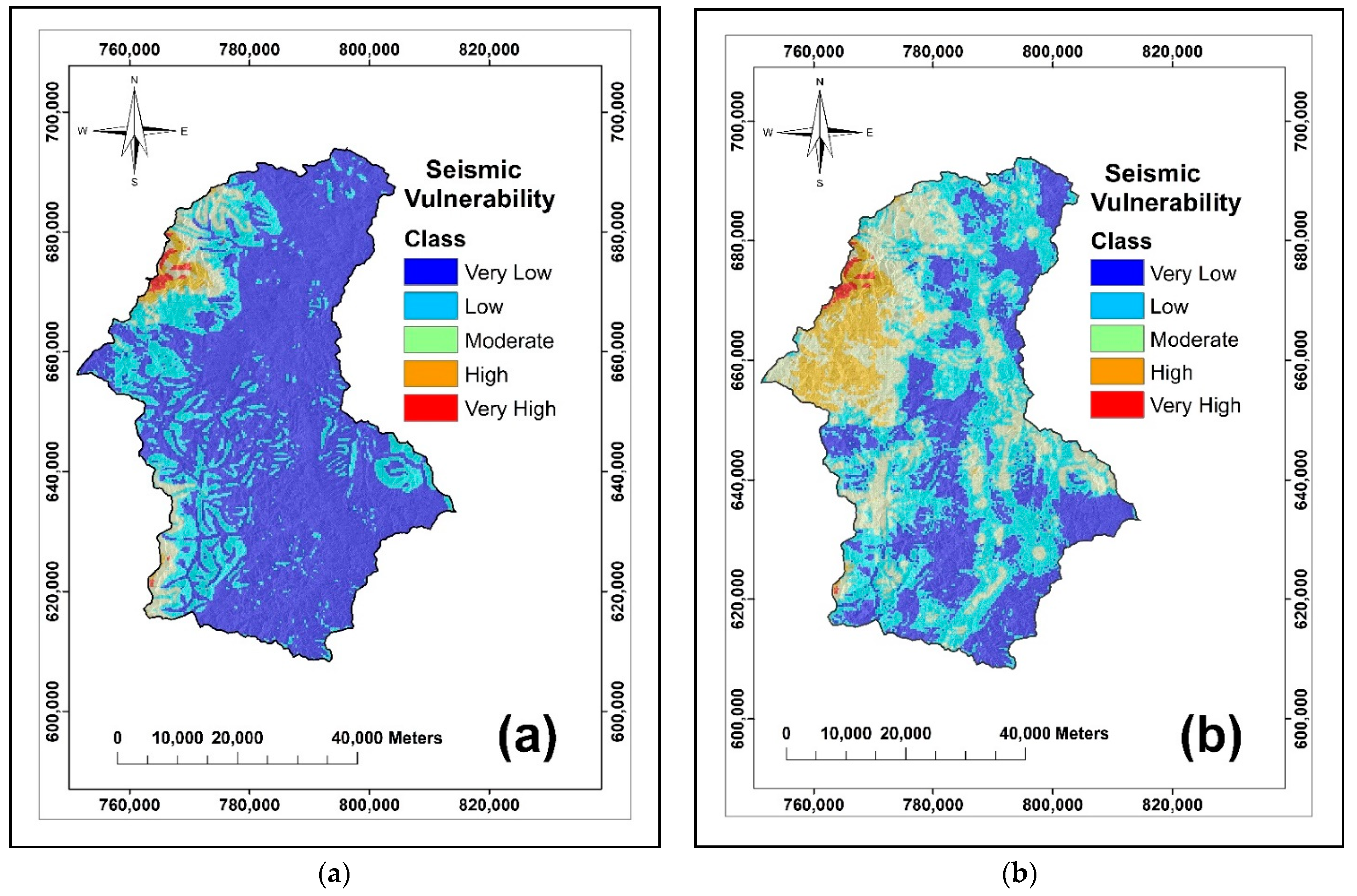
3.2. Seismic Vulnerability Maps

Two seismic vulnerability maps were produced separately using FR-IoE and (FR-IoE) AHP models. The maps were presented in the form of vulnerability index ranging from 0.343–3.863 for the FR-IoE model and between 0.069–0.539 for the (FR-IoE) AHP model. The maps were classified into five vulnerability classes following methodologies from [91,92,93,94,95]. The selection of the classification method was based on the distribution of the vulnerability indexes [37]. As the histogram skewed positively for both models, the natural break classifier was applied to the models [96]. The final vulnerability maps using the two models with five vulnerability classes are shown in Figure 3a,b.
To examine the distribution of past seismic data along with the five vulnerability classes, seismic activities density analysis was performed following methodologies from [97,98] as shown in Table 5.
It was shown that 71.428% of the total area of seismic vulnerability map produced using the FR-IoE model have a very low seismic vulnerability; 21.900% of the areas fall under low vulnerability zones. Moderate vulnerability areas constituted 4.926% of the total area. The high and very high vulnerability zones contributed 1.378% and 0.548% of the total area, respectively. Overall, 15.000% of the total past seismic activities fall in the very high and high seismic vulnerability areas. Moderate vulnerability zones made up 20.000% of the past seismic activities. Low and very low seismic zones contributed 65.000% of the total past seismic activities. High seismic activity density ratios were observed for high and very high vulnerability areas at 7.254 and 9.119, respectively.
The seismic vulnerability map produced using the (FR-IoE) AHP model displayed very low and low seismic vulnerability for 30.360% and 40.049% of the total area, respectively. Moderate vulnerability areas made up 21.314% of the total area. The high and very high vulnerability zones accounted for 7.703% and 0.575% of the total area, respectively; 51.667% of the total past seismic activities fall in the very high and high vulnerability areas. Moderate vulnerability zones made up 26.667% of the past seismic activities. Low and very low seismic zones contributed 21.666% of the total past seismic activities. Similar to the FR-IoE model, high seismic activity density ratios were observed for high and very high vulnerability areas at 8.697 and 6.059, respectively. According to [13], an ideal susceptibility map has the events (e.g., landslides) density values increasing from low to higher-tiered class. Based on Table 5, the past seismic activity density is gradually increased from low to high vulnerability class which satisfied the analysis.

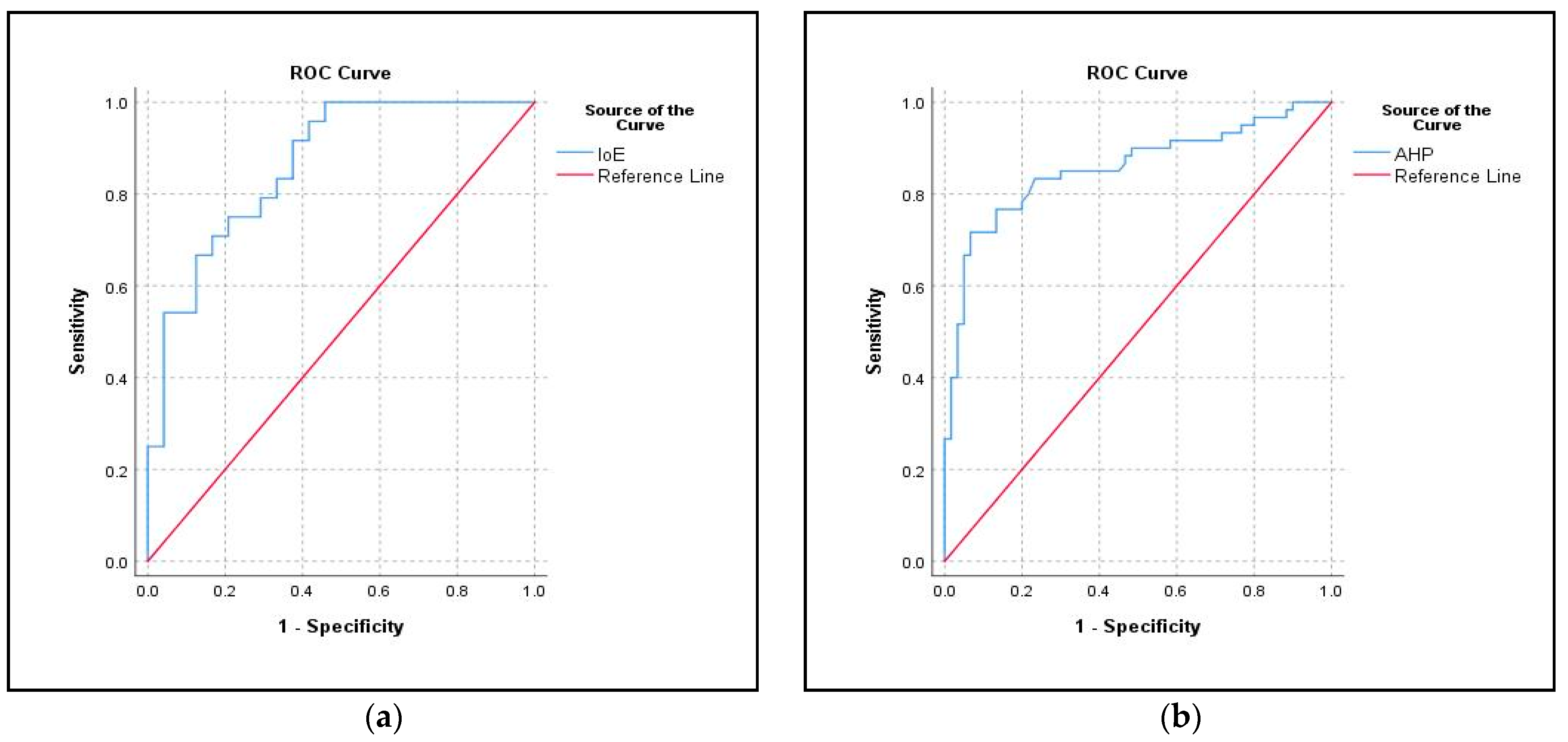
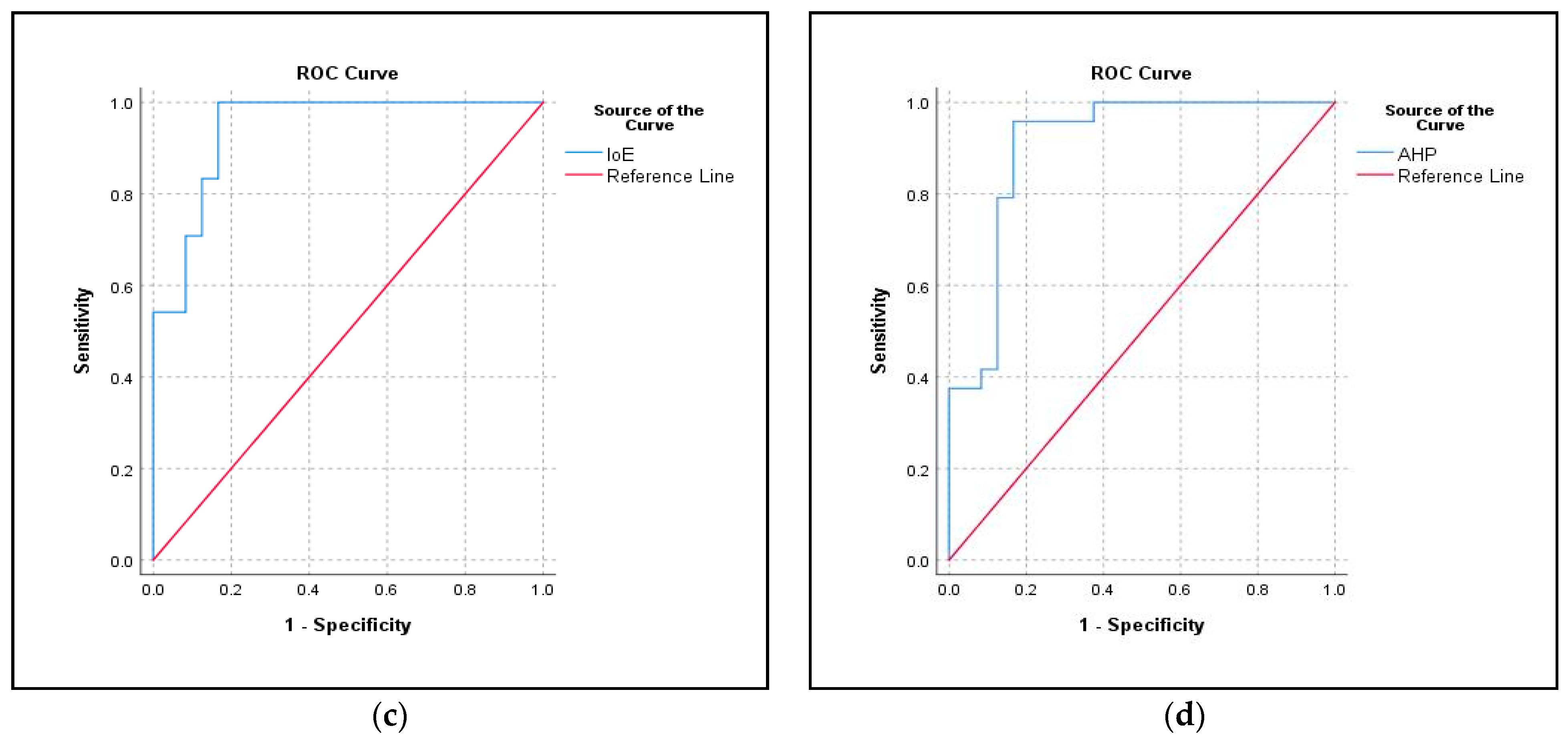
3.3. Model Validation

To determine the models’ quality and to validate the models’ reliability, the seismic vulnerability maps produced were checked using areas under the ROC curves based on guides from previous research such as [10,12,13,98,99,100]. According to [101], the ROC method represents different accuracy values obtained against the whole range of possible threshold values of the functions and serves as a global accuracy statistic for the model. The ROC curve is mapped for the sensitivity of the model against 1-specificity [102,103]. ROC provided the diagnostic accuracy of the model in the form of AUC values as shown in Table 6. For model validation, success rate and prediction rate curves were created by comparing the past seismic activities with the seismic vulnerability maps [10,21]. The ROC curves were computed using SPSS software as shown in Figure 4.
The FR-IoE and model had success and a prediction rate of 0.853 and 0.863, respectively, while (FR-IoE) AHP reported a success rate and prediction rate of 0.856 and 0.906, respectively. AUC values range from 0 to 1; a value of 0 indicates a perfectly poor model, a value of 1 reflects a perfectly accurate model and a value of 0.5 suggests no discrimination or no class separation existed in the model [104]. Reference [105] stated a guide for interpreting AUC values for a model as follows; 0.90–1 as excellent, 0.80–0.90 as good, 0.70–0.80 as fair, 0.60–0.70 as poor and 0.50–0.60 as fail. In this study, the (FR-IoE) AHP model was evaluated to have the highest accuracy. The models used for this study all have asymptotic significance probability 0.00 with lower and upper boundaries of the 95% asymptotic confidence interval of ≥ 0.762 for both models, indicating statistical significance [12].

4. Discussion

4.1. Tectonic Settings and Their Importance to Seismic Vulnerability Assessment in Ranau, Sabah

Vulnerability assessment in Ranau and particularly Sabah is very important due to its ‘risky’ location on the Sunda Plate and a tectonically dynamic margin of Borneo where it is surrounded by active plates of the Sunda, Indo-Australian, and Philippines Sea plates with a highly concentrated distribution of seismic activities around this region [106,107]. Through the Philippine-Pacific, the effects of the movements of the plates at the rate of ~10 cm/year against the moving Eurasian plate at the rate of ~5 cm/year placed Sabah under a west-northwest–east-southeast (WNW–ESE) compressive stress regime along with north-east–south-west (NE–SW) trending active thrust faults and north-west-south-east (NW-SE) trending active strike-slip faults [32]. Effects from seismic activities from south Indonesia are higher due to the Sunda plate [5,108,109,110]. Since 1973, multiple earthquakes between magnitude 7.5 to 9.0 have occurred in the tectonic Sunda Plate boundaries that were induced by the Sunda Trench and Manila Trench on the Sunda Plate boundary and by the Molucca Sea, Banda Sea, Timor and Bird’s Head plates in the southeast [4,111]. In short, Sabah is ‘sitting’ on the movement of the major plates. According to [32], about 65 local light to moderate seismic activities with magnitude >3 were recorded on USGS and Incorporated Research Institutions for Seismology (IRIS) earthquake database from 1900 to 2016 onshore or within the waters of Sabah. The records were limited due to the detection by older seismographs in Sabah. Installation of new seismographs in Sabah in 2009 recorded a hike in seismic activities. In the year 2015 solely, MetMalaysia recorded 155 small earthquakes with magnitude >2 in Sabah. These earthquakes were concentrated around the Lahad Datu-Kunak and Kundasang-Ranau areas. The records proved that the region is tectonically active and, in the future, an earthquake with a large magnitude as compared to the 2015 6.0 Mw Ranau earthquake might occur. Apart from slope angle, elevation and distance from buildings factors, faulty lines are also concentrated in the same areas in Ranau with FR = 1.646 and FR = 1.409 for both distances‘ 1 km’ and ‘2 km’ from the faults. The final vulnerability maps produced also showed that high and very high vulnerability areas ‘coincide’ with the areas that are concentrated by these four factors with the highest entropy values. Thus, any major movement from plates that exist in these areas can induce a major earthquake in the future that can bring extensive damage to the areas.

4.2. Seismic Vulnerability Studies in the Study Area

Past research on seismic vulnerability in Sabah such as [7,112,113,114,115] only focused on buildings or physical vulnerability rather than implementing the combination of various indicators such as physical (e.g. buildings, buildings’ materials and other man-made infrastructures), economy (Gross Domestic Product (GDP), wealth of households), environmental (slope, elevation) and social (population, age) indicators in vulnerability mapping [16,21,116]. Reference [7] for example, evaluated 54 buildings in 12 districts of Sabah to determine their structural performance level and structural deficiency. They suggested an appropriate retrofitting plan for buildings under the risk of damages based on the predicted intensity of seismic activities from the outcomes of their study. Reference [115] investigated vulnerability of public buildings in Sabah for low, medium, and high-rise buildings through eight reinforced concrete buildings. They used finite element modeling (FEM) and applied different intensities of earthquake load to analyze the maximum allowable earthquake load intensities for the buildings. The model simulations showed that if any low to medium earthquake intensity is to occur, the event would mostly incur moderate damage to the buildings in the study. These studies were very much limited and focusing on one type of factor only which is the structural component of the seismic vulnerability study in the study area.
Thus, in this study, an attempt was made to model seismic vulnerability in Ranau, Sabah, using methodologies undertaken by [10,11,12,13,96,97,117] by incorporating two indicators; physical and environmental indicators. Two different hybrid models; FR-IoE and (FR-IoE) AHP which originated from three models; FR, IoE and AHP were used to assess seismic vulnerability in Ranau district, Sabah, using previous records of seismic activities in the region by considering nine factors as the input data for the model construction. All the data were processed in a GIS environment which has been regarded as an excellent tool in spatial management and data manipulation [12]. Studies on past research [118,119,120,121,122,123] showed that they succeeded in modeling various natural disasters (e.g., landslides, floods, volcanic eruptions, forest fire, tsunamis) using FR or IoE or the combination of both and AHP either for mitigation, susceptibility, vulnerability, hazard or risk purposes with good model performances.

4.3. Comparisons with Past Research on the Seismic Vulnerability Assessment

Although seismic vulnerability assessment using various indicators with similar approaches has never been carried out in the study area, various research projects internationally have been undertaken concerning seismic vulnerability assessment. [25] for example used FR, DT, RF to map the seismic vulnerability of Gyeongju, South Korea, and compared the accuracies of the three models using 18 factors. They found out that the peak ground acceleration (PGA) and distance to the epicenter have the highest influences on seismic vulnerability in the DT and RF models while altitude had the greatest impact in the FR model. Their analysis showed the RF model to have the highest functional performances with success and prediction rates of 1.000 and 0.949, followed by the DT model with 0.899 and 0.851, and the FR model with 0.661 and 0.655 for success and prediction rates, respectively.
Reference [21] used LR and four kernel models of SVM; linear (L), polynomial (P), radial basis function (RBF), and sigmoid (S) for seismic vulnerability purposes, also using 18 factors. The success rates observed were 0.652, 0.649, 0.842, 0.998, and 0.630 with the prediction rates of 0.714, 0.651, 0.804, 0.919, and 0.629 for LR, SVM-L, SVM-P, SVM-RBF and SVM-S models, respectively. The highest model’s performance was obtained by RBF-SVM. The evaluation of the factors used to construct the LR model showed that building age, distance to roads, and construction materials were less significant in the seismic vulnerability of the study area.
Reference [124] employed LogitBoost, logistic model tree (LMT), and LR to map and analyze the seismic vulnerability in southeast Korea using 15 related factors. The AUC values computed were were 0.769, 0.851, and 0.749, respectively, for LogitBoost, LMT and LR models. They found that factors such as PGA and distance from the epicenter strongly influenced the seismic vulnerability of the study area.
Reference [17] combined five different models (OWA, fuzzy, AHP, ANP and LR) as four hybrid models (A-fuzzy, A-OWA, Fuzzy-LR and OWA-LR) to improve the accuracy of seismic vulnerability mapping in their study area of Sanandaj City, Iran using 15 factors. They found that the dominating factors were population density and distance from the fault. Their validation results showed that A-OWA and OWA-LR models provided the best model performances with AUC values of 0.855 and 0.900 respectively. Based on their results, they suggested the implementation of hybrid models to eliminate unreliable results that existed in individual models.
These research works used various models or combinations of the models for seismic vulnerability assessment in their respective areas of interest. The number of factors they chose in seismic vulnerability mapping and the factor(s) that have a strong influence on seismic vulnerability in their study areas were also different for each study. From all the factors used in these researches, factors such as altitude, the existence of buildings and distance from faults consistently appeared to be highly influenced in seismic vulnerability assessment of the study areas. These findings have mostly influenced the factors chosen for this study and should be used as an important reference for future related studies. The seismic vulnerability mapping result could also be improved by exploring alternatives such as hybrid models of various individual models, particularly the combination of the traditional method such as AHP with deep learning models such as ANN or RF as shown by [17].

4.4. Relevance and Output of the Studies

Reviews from international literature showed that few works have been undertaken concerning earthquake or seismic vulnerability using the combination of FR-IoE. Most of the research used FR alone for earthquake or seismic vulnerability assessment [21]. In this study, the combination between FR-IoE results with AHP experimented with the main idea was to minimize bias that existed in the decision-making process from AHP methodologies. The performances of both models were then compared based on the final seismic vulnerability index maps. The model validation using areas under the ROC curves showed accuracy level between good to excellent were achieved for both models with AUC values ≥0.853 for both success and prediction rate with the (FR-IoE) AHP model showing the highest accuracy for both success and prediction rate. From the results, it can be hypothesized that the methodologies and result of AHP could be boosted by integrating the AHP process with other decision-making model/s. For future researches, an old method such as AHP can be combined as a hybrid with machine learning methods such as SVM, ANN, RF, and Naïve Bayes to analyze the performances of these models combination in natural hazard analysis. From the nine factors used in this study, slope and altitude factors were found to be the most significant factors influencing the seismic vulnerability in Ranau with Wj = 2.118 and Wj = 0.627 for slope and altitude factors respectively. Both final seismic vulnerability maps produced consistent output in which very high and high vulnerability areas were concentrated on the northeast part of Ranau where Mount Kinabalu and Crocker Range are located.

5. Conclusions

This study implemented three models; FR, IoE and AHP in seismic vulnerability assessment of Ranau, Sabah. Nine factors that are related to physical and environmental indicators were used in this study including slope, altitude, distance from buildings, distance from faulty lines, distance from rivers, lithology, distance from tracks, distance from roads and distance from streams factors. The results showed that slope, altitude, distance from buildings and distance from fault lines were the most significant factors in seismic vulnerability assessment of the study area with distance from streams evaluated to be less likely to influence the seismic vulnerability in Ranau, Sabah. The researchers acknowledged that there were limited numbers of conditional factors or parameters used in this study. However, as a pilot study, the numbers of conditional factors used were enough to access seismic vulnerability in the study area. It is recommended that future studies of seismic vulnerability should consider other factors such as utilities (e.g., electric, gas, water, and telecommunications), population, and land-cover/land-use data. The seismic vulnerability map produced for the study area would be useful for planners and decision-makers to mitigate any potential large magnitude earthquake in the study area to reduce damage and fatalities incurred by such earthquakes based on the identification of areas with high and very high vulnerability in Ranau, Sabah. A future research direction should include seismic hazard properties such as ground motion (e.g., PGA, peak ground velocity (PGV)), fault rupture and soil liquefaction [125] to combine with a seismic vulnerability map of the area to produce a complete final seismic risk map.

Author Contributions

Janatul Aziera binti Abd Razak involved in the data processing and analysis and wrote the article. Shuib bin Rambat organized the research framework and aided in proposing the research concept. Faizah binti Che Ros involved in data analysis. Zhongchao Shi review the article. Saiful Amri bin Mazlan review and proofread the article. All authors have read and agreed to the published version of the manuscript.

Funding

This research was funded by Universiti Teknologi Malaysia (UTM), grant number Q.K130000.3843.20J00.

Acknowledgments

The authors thank Department of Survey and Mapping Malaysia (JUPEM), Malaysian Meteorological Department (MetMalaysia) and Department of Mineral and Geoscience Malaysia (JMG) for providing data used in this study. The authors are also grateful toward United States Geological Survey (USGS), Incorporated Research Institutions for Seismology (IRIS), European Space Agency (ESA) for their open access data.

Conflicts of Interest

The authors declare no conflict of interest.

References

  1. Yan, A.S.; Saim Suratman, A.L. Study on the Seismic and Tsunami Hazards and Risks in Malaysia. In Report on the Geological and Seismotectonic Information of Malaysia, Kuala Lumpur, Ministry of Natural Resources and Environment; 2006. [Google Scholar]
  2. Bakar, R.B.; Jamaluddin, T.A.; Ramli, Z.; Mohamad, Z.; Tongkul, F. Remotely Sensed Geospatial Analysis towards Disaster Preparedness: A Case Study in Malaysia Tectonically Active Earthquake Zone, Ranau, Sabah. FIG Work. Week. Recov. Disaster. 2016, 15, 868–877. [Google Scholar]
  3. Malaysian Meteorological Department. Seismicity in Malaysia. Available online: http://www.met.gov.my/in/web/metmalaysia/education/earthquakeandtsunami/seismicityinmalaysiaandaroundtheregion (accessed on 20 December 2017).
  4. Cheng, K.H. Plate Tectonics and Seismic Activities in Sabah Area. Trans. Sci. Technol. 2016, 3, 47–58. [Google Scholar]
  5. Khalil, A.E.; Abir, I.A.; Hafiez, H.E.A.; Ginsos, H.; Khan, M.S. Probabilistic Seismic Hazards Assessments of Sabah, East Malaysia: Accounting for Local Earthquake Activity Near Ranau. J. Geophys. Eng. 2017, 15, 13–25. [Google Scholar] [CrossRef] [Green Version]
  6. Harith, N.S.H.; Adnan, A.; Tongkul, F.; Shoushtari, A.V. Analysis on Earthquake Databases of Sabah Region and Its Application for Seismic Design. Int. J. Civil. Eng. Geo-Environ. 2017, 8, 1–5. [Google Scholar]
  7. Mansor, M.N.A.; Siang, L.C.; Ahwang, A.; Saadun, M.A.; Dumatin, J. Vulnerability Study of Existing Buildings Due to Seismic Activities in Sabah. ISSN:21802742. Available online: http://ijceg.ump.edu.my (accessed on 21 April 2021).
  8. Sali, A.; Zainal, D.; Ahmad, N.T.; Omar, M.F. Satellite Application for Felt Earthquake Events in Sabah, Malaysia. Int. J. Environ. Sci. Dev. 2017, 8, 153. [Google Scholar] [CrossRef] [Green Version]
  9. Devkota, K.C.; Regmi, A.D.; Pourghasemi, H.R.; Yoshida, K.; Pradhan, B.; Ryu, I.C.; Dhital, M.R.; Althuwaynee, O.F. Landslide Susceptibility Mapping Using Certainty Factor, Index of Entropy and Logistic Regression Models in GIS And Their Comparison at Mugling–Narayanghat Road Section in Nepal Himalaya. Nat. Hazar. 2013, 65, 135–165. [Google Scholar] [CrossRef]
  10. Jaafari, A.; Najafi, A.; Pourghasemi, H.R.; Rezaeian, J.; Sattarian, A. GIS-based Frequency Ratio and Index of Entropy Models for Landslide Susceptibility Assessment in the Caspian Forest, Northern Iran. Int. J. Environ. Sci. Technol. 2014, 11, 909–926. [Google Scholar] [CrossRef] [Green Version]
  11. Liu, J.; Duan, Z. Quantitative Assessment of Landslide Susceptibility Comparing Statistical Index, Index of Entropy, And Weights of Evidence in the Shangnan Area, China. Entropy 2018, 20, 868. [Google Scholar] [CrossRef] [Green Version]
  12. Park, S.; Choi, C.; Kim, B.; Kim, J. Landslide Susceptibility Mapping Using Frequency Ratio, Analytic Hierarchy Process, Logistic Regression, and Artificial Neural Network Methods at the Inje Area, Korea. Environ. Earth Sci. 2013, 68, 1443–1464. [Google Scholar] [CrossRef]
  13. Pradhan, B.; Lee, S. Delineation of Landslide Hazard Areas on Penang Island, Malaysia, by Using Frequency Ratio, Logistic Regression, and Artificial Neural Network Models. Environ. Earth Sci. 2010, 60, 1037–1054. [Google Scholar] [CrossRef]
  14. Cabal, A.; Coulet, C.; Erlich, M.; Cossalter, A.; David, E.; Sauvaget, P.; Maria Polese, A.E.E.; Zuccaro, G.; Alten, K.; Steinnocher, K.; et al. Existing Hazard and Vulnerability/Losses Models. Available online: https://www.researchgate.net/profile/Maria-Polese/publication/283307151_Models_for_MultiSectoral_Consequences_Existing_hazard_and_vulnerability_losses_models/links/56372f7e08ae88cf81bd4f89/Models-for-Multi-Sectoral-Consequences-Existing-hazard-and-vulnerability-losses-models.pdf (accessed on 6 April 2021).
  15. Van Westen, C.J. Introduction to Exposure, Vulnerability and Risk Assessment. 2020. Available online: http://www.charim.net/methodology/51 (accessed on 7 April 2021).
  16. Duzgun, H.S.B.; Yucemen, M.S.; Kalaycioglu, H.S.; Celik, K.; Kemec, S.; Ertugay, K.; Deniz, A. An Integrated Earthquake Vulnerability Assessment Framework for Urban Areas. Nat. Hazar. 2011, 59, 917–947. [Google Scholar] [CrossRef]
  17. Yariyan, P.; Avand, M.; Soltani, F.; Ghorbanzadeh, O.; Blaschke, T. Earthquake Vulnerability Mapping Using Different Hybrid Models. Symmetry 2020, 12, 405. [Google Scholar] [CrossRef] [Green Version]
  18. Jena, R.; Pradhan, B.; Naik, S.P.; Alamri, A.M. Earthquake Risk Assessment in NE India Using Deep Learning and Geospatial Analysis. Geosci. Front. 2021, 12, 10111. [Google Scholar] [CrossRef]
  19. Toyfur, M.F.; Pribadi, K.S.; Wibowo, S.S.; Sengara, I.W. Vulnerability Factor in Earthquake Risk Assessment Model for Roads in Indonesia. EDP Sci. MATEC Web Conf. 2018, 229, 03009. [Google Scholar] [CrossRef] [Green Version]
  20. Nazmfar, H.; Saredeh, A.; Eshgi, A.; Feizizadeh, B. Vulnerability Evaluation of Urban Buildings to Various Earthquake Intensities: A Case Study of the Municipal Zone 9 of Tehran. Hum. Ecol. Risk Assess. Int. J. 2019, 25, 455–474. [Google Scholar] [CrossRef]
  21. Han, J.; Park, S.; Kim, S.; Son, S.; Lee, S.; Kim, J. Performance of Logistic Regression and Support Vector Machines for Seismic Vulnerability Assessment and Mapping: A Case Study of the 12 September 2016 ML5. 8 Gyeongju Earthquake, South Korea. Sustainability 2019, 11, 7038. [Google Scholar] [CrossRef] [Green Version]
  22. Saputra, A.; Rahardianto, T.; Revindo, M.D.; Delikostidis, I.; Hadmoko, D.S.; Sartohadi, J.; Gomez, C. Seismic Vulnerability Assessment of Residential Buildings using Logistic Regression and Geographic Information System (GIS) in Pleret Sub District (Yogyakarta, Indonesia). Geoenviron. Disasters 2017, 4, 1–33. [Google Scholar] [CrossRef] [Green Version]
  23. Alizadeh, M.; Alizadeh, E.; Asadollahpour, K.S.; Shahabi, H.; Beiranvand Pour, A.; Panahi, M.; Bin Ahmad, B.; Saro, L. Social Vulnerability Assessment Using Artificial Neural Network (ANN) Model for Earthquake Hazard in Tabriz City, Iran. Sustainability 2018, 10, 3376. [Google Scholar] [CrossRef] [Green Version]
  24. Alizadeh, M.; Ngah, I.; Hashim, M.; Pradhan, B.; Pour, A.B. A Hybrid Analytic Network Process and Artificial Neural Network (ANP-ANN) Model for Urban Earthquake Vulnerability Assessment. Remote Sens. 2018, 10, 975. [Google Scholar] [CrossRef] [Green Version]
  25. Han, J.; Kim, J.; Park, S.; Son, S.; Ryu, M. Seismic Vulnerability Assessment and Mapping of Gyeongju, South Korea Using Frequency Ratio, Decision Tree, and Random Forest. Sustainability 2020, 12, 7787. [Google Scholar] [CrossRef]
  26. Lee, S.; Panahi, M.; Pourghasemi, H.R.; Shahabi, H.; Alizadeh, M.; Shirzadi, A.; Khosravi, K.; Melesse, A.M.; Yekrangnia, M.; Rezaie, F.; et al. SEVUCAS: A Novel GIS-Based Machine Learning Software for Seismic Vulnerability Assessment. Appl. Sci. 2019, 9, 3495. [Google Scholar] [CrossRef] [Green Version]
  27. Chen, W.; Li, W.; Hou, E.; Bai, H.; Chai, H.; Wang, D.; Cui, X.; Wang, Q. Application of Frequency Ratio, Statistical Index, and Index of Entropy Models and Their Comparison in Landslide Susceptibility Mapping for the Baozhong Region of Baoji, China. Arab. J. Geosci. 2015, 8, 1829–1841. [Google Scholar] [CrossRef]
  28. Wang, Y.; Fang, Z.; Hong, H.; Costache, R.; Tang, X. Flood Susceptibility Mapping by Integrating Frequency Ratio and Index of Entropy with Multilayer Perceptron and Classification and Regression Tree. J. Environ. Manag. 2021, 289, 112449. [Google Scholar] [CrossRef] [PubMed]
  29. Wang, Q.; Li, W.; Yan, S.; Wu, Y.; Pei, Y. GIS Based Frequency Ratio and Index of Entropy Models to Landslide Susceptibility Mapping (Daguan, China). Environ. Earth Sci. 2016, 75, 780. [Google Scholar] [CrossRef]
  30. Ranau District Office. Latar Belakang Daerah Ranau. 2019. Available online: http://ww2.sabah.gov.my/pd.rnu/sejarah.html (accessed on 3 January 2019).
  31. Department of Statistics, Malaysia. Population Distribution by Local Authority Areas and Mukims. 2010. Available online: https://www.mycensus.gov.my/index.php/census-product/publication/census-2010/681-population-distribution-by-local-authority-and-mukims-2010 (accessed on 2 January 2019).
  32. Tongkul, F. Active Tectonics in Sabah—Seismicity and Active Faults. Bull. Geol. Soc. Malays. 2017, 64, 27–36. [Google Scholar] [CrossRef] [Green Version]
  33. Tongkul, F. The 2015 Ranau Earthqauke: Cause and Impact. Sabah Soc. J. 2016, 32, 1–28. [Google Scholar]
  34. Sarris, A.; Loupasakis, C.; Soupios, P.; Trigkas, V.; Vallianatos, F. Earthquake Vulnerability and Seismic Risk Assessment of Urban Areas in High Seismic Regions: Application to Chania City, Crete Island, Greece. Nat. Hazards 2010, 54, 395–412. [Google Scholar] [CrossRef]
  35. Caliskan, S.; Taubenböck, H.; Hinz, S.; Roth, A. Earthquake Vulnerability Indicators and Vulnerability Assessment Using Remote Sensing, Istanbul. 2006. 1st EARSeL Workshop SIG Urban. Remote Sens. Berlin, Germany. Available online: https://www.researchgate.net/publication/224798942 (accessed on 8 April 2021).
  36. Aliabadi, S.F.; Sarsangi, A.; Modiri, E. The Social and Physical Vulnerability Assessment of Old Texture against Earthquake (Case Study: Fahadan District in Yazd City). Arab. J. Geosci. 2015, 8, 10775–10787. [Google Scholar] [CrossRef]
  37. Ayalew, L.; Yamagishi, H. The Application of GIS-Based Logistic Regression for Landslide Susceptibility Mapping in The Kakuda-Yahiko Mountains, Central Japan. Geomorphology 2005, 65, 15–31. [Google Scholar] [CrossRef]
  38. Pavić, G.; Bulajić, B.; Hadzima-Nyarko, M. The Vulnerability of Buildings from the Osijek Database. Front. Built. Environ. 2019, 5, 66. [Google Scholar] [CrossRef] [Green Version]
  39. Kontogianni, V.; Pytharouli, S.; Stiros, S. Ground Subsidence, Quaternary Faults and Vulnerability of Utilities and Transportation Networks in Thessaly, Greece. Environ. Geol. 2007, 52, 1085–1095. [Google Scholar] [CrossRef]
  40. Kermanshah, A.; Derrible, S. A Geographical and Multi-Criteria Vulnerability Assessment of Transportation Networks against Extreme Earthquakes. Reliabil. Eng. Syst. Safety 2016, 153, 39–49. [Google Scholar] [CrossRef]
  41. Pachauri, A.K.; Pant, M. Landslide Hazard Mapping Based on Geological Attributes. Eng. Geol. 1992, 32, 81–100. [Google Scholar] [CrossRef]
  42. Rodrıguez, C.E.; Bommer, J.J.; Chandler, R.J. Earthquake-induced Landslides: 1980–1997. Soil Dynam. Earthq. Eng. 1999, 18, 325–346. [Google Scholar] [CrossRef]
  43. Bommer, J.J.; Rodrı́guez, C.E. Earthquake-induced Landslides in Central America. Eng. Geol. 2002, 63, 189–220. [Google Scholar] [CrossRef]
  44. Ren, D.; Wang, J.; Fu, R.; Karoly, D.J.; Hong, Y.; Leslie, L.M.; Fu, C.; Huang, G. Mudslide-caused Ecosystem Degradation Following Wenchuan Earthquake 2008. Geophys. Res. Lett. 2009, 36. [Google Scholar] [CrossRef]
  45. Wang, H.B.; Sassa, K.; Xu, W.Y. Analysis of a Spatial Distribution of Landslides Triggered by the 2004 Chuetsu Earthquakes of Niigata Prefecture, Japan. Nat. Hazards 2007, 41, 43. [Google Scholar] [CrossRef]
  46. USGS. Ground Shaking Simulations: Background. 2020. Available online: https://earthquake.usgs.gov/education/shakingsimulations/background.php (accessed on 13 December 2020).
  47. Tang, C.; Zhu, J.; Li, W.L.; Liang, J.T. Rainfall-triggered Debris Flows Following the Wenchuan Earthquake. Bull. Eng. Geol. Environ. 2009, 68, 187–194. [Google Scholar] [CrossRef]
  48. Ujiie, K.; Kimura, G. Earthquake Faulting in Subduction Zones: Insights from Fault Rocks in Accretionary Prisms. Prog. Earth Planet. Sci. 2014, 1, 7. [Google Scholar] [CrossRef] [Green Version]
  49. Earle, S. Physical Geology. Victoria, B.C.: BCcampus. 2015. Available online: https://opentextbc.ca/geology/ (accessed on 22 February 2021).
  50. Potter, S.H.; Becker, J.S.; Johnston, D.M.; Rossiter, K.P. An Overview of the Impacts of the 2010–2011 Canterbury Earthquakes. Int. J. Disaster Risk Reduct. 2015, 14, 6–14. [Google Scholar] [CrossRef] [Green Version]
  51. Jibson, R.W. Methods for Assessing the Stability of Slopes During Earthquakes—A Retrospective. Eng. Geol. 2011, 122, 43–50. [Google Scholar] [CrossRef]
  52. Hack, R.; Alkema, D.; Kruse, G.A.; Leenders, N.; Luzi, L. Influence of Earthquakes on the Stability of Slopes. Eng. Geol. 2007, 91, 4–15. [Google Scholar] [CrossRef]
  53. Umar, Z.; Pradhan, B.; Ahmad, A.; Jebur, M.N.; Tehrany, M.S. Earthquake Induced Landslide Susceptibility Mapping Using an Integrated Ensemble Frequency Ratio and Logistic Regression Models in West Sumatera Province, Indonesia. Catena 2014, 118, 124–135. [Google Scholar] [CrossRef]
  54. Lee, S.; Pradhan, B. Landslide hazard mapping at Selangor, Malaysia using frequency ratio and logistic regression models. Landslides 2007, 4, 33–41. [Google Scholar] [CrossRef]
  55. Nohani, E.; Moharrami, M.; Sharafi, S.; Khosravi, K.; Pradhan, B.; Pham, B.T.; Lee, S.; Melesse, A. Landslide susceptibility mapping using different GIS-based bivariate models. Water 2019, 11, 1402. [Google Scholar] [CrossRef] [Green Version]
  56. Yalcin, A.; Reis, S.; Aydinoglu, A.C.; Yomralioglu, T. A GIS-based comparative study of frequency ratio, analytical hierarchy process, bivariate statistics and logistics regression methods for landslide susceptibility mapping in Trabzon, NE Turkey. Catena 2011, 85, 274–287. [Google Scholar] [CrossRef]
  57. Regmi, A.D.; Devkota, K.C.; Yoshida, K.; Pradhan, B.; Pourghasemi, H.R.; Kumamoto, T.; Akgun, A. Application of Frequency Ratio, Statistical Index, and Weights-of-Evidence Models and Their Comparison in Landslide Susceptibility Mapping in Central Nepal Himalaya. Arab. J. Geosci. 2014, 7, 725–742. [Google Scholar] [CrossRef]
  58. Bednarik, M.; Yilmaz, I.; Marschalko, M. Landslide Hazard and Risk Assessment: A Case Study from the Hlohovec–Sered’landslide Area in South-west Slovakia. Nat. Hazards 2012, 64, 547–575. [Google Scholar] [CrossRef]
  59. Can, T.; Nefeslioglu, H.A.; Gokceoglu, C.; Sonmez, H.; Duman, T.Y. Susceptibility Assessments of Shallow Earthflows Triggered by Heavy Rainfall at Three Catchments by Logistic Regression Analyses. Geomorphology 2005, 72, 250–271. [Google Scholar] [CrossRef]
  60. Constantin, M.; Bednarik, M.; Jurchescu, M.C.; Vlaicu, M. Landslide Susceptibility Assessment Using the Bivariate Statistical Analysis and The Index of Entropy in the Sibiciu Basin (Romania). Environ. Earth Sci. 2011, 63, 397–406. [Google Scholar] [CrossRef]
  61. Dai, F.C.; Lee, C.F.; Zhang, X.H. GIS-Based Geo-Environmental Evaluation for Urban Land-Use Planning: A Case Study. Eng. Geol. 2001, 61, 257–271. [Google Scholar] [CrossRef]
  62. Sharma, L.P.; Patel, N.; Ghose, M.K.; Debnath, P. Influence of Shannon’s Entropy on Landslide-causing Parameters for Vulnerability Study and Zonation—A Case Study in Sikkim, India. Arab. J. Geosci. 2012, 5, 421–431. [Google Scholar] [CrossRef]
  63. Bednarik, M.; Magulová, B.; Matys, M.; Marschalko, M. Landslide Susceptibility Assessment of the Kraľovany–Liptovský Mikuláš Railway Case Study. Phys. Chem. Earth Parts A/B/C 2010, 35, 162–171. [Google Scholar] [CrossRef]
  64. Saaty, T.L. A Scaling Method for Priorities in Hierarchical Structures. J. Math. Psychol. 1977, 15, 234–281. [Google Scholar] [CrossRef]
  65. Rezaei, A.; Tahsili, S. Urban Vulnerability Assessment Using AHP. Adv. Civil. Eng. 2018, 62. [Google Scholar] [CrossRef] [Green Version]
  66. Saaty, T.L. The Analytic Hierarchy Process; McGraw-Hill: New York, NY, USA, 1980. [Google Scholar]
  67. Saaty, L. An Analytical Hierarchy and Network Processes Approach for the Measurement in Tangible Criteria and for Decision Making; Multiple Criteria Decision. State Art Survey 2005, 345–406. [Google Scholar]
  68. Keshavarzi, A.; Sarmadian, F.; Heidari, A.; Omid, M. Land Suitability Evaluation Using Fuzzy Continuous Classification (A Case Study: Ziaran Region). Mod. Appl. Sci. 2010, 4, 72. [Google Scholar] [CrossRef] [Green Version]
  69. Saaty, T.L. Decision-making with the AHP: Why is the Principal Eigenvector Necessary? Eur. J. Oper. Res. 2003, 145, 85–91. [Google Scholar] [CrossRef]
  70. Vahidnia, M.H.; Alesheikh, A.; Alimohammadi, A.; Bassiri, A. Fuzzy analytical hierarchy process in GIS application. Int. Arch. Photogram. Remote Sens. Spatial Inform. Sci. 2008, 37, 593–596. [Google Scholar]
  71. Alizadeh, M.; Hashim, M.; Alizadeh, E.; Shahabi, H.; Karami, M.R.; Beiranvand Pour, A.; Zabihi, H. Multi-Criteria Decision Making (MCDM) Model for Seismic Vulnerability Assessment (SVA) of Urban Residential Buildings. ISPRS Int. J. Geo-Inform. 2018, 7, 444. [Google Scholar] [CrossRef] [Green Version]
  72. Saaty, T.L. What is the Analytic Hierarchy Process? In Mathematical Models for Decision; Springer: Berlin/Heidelberg, Germany, 1988; pp. 109–121. [Google Scholar]
  73. Saaty, T.L. How to Make a Decision: The Analytic Hierarchy Process. Eur. J. Oper. Res. 1990, 48, 9–26. [Google Scholar] [CrossRef]
  74. Saaty, R.W. The Analytic Hierarchy Process—What It Is and How It Is Used. Math. Model. 1987, 9, 161–176. [Google Scholar] [CrossRef] [Green Version]
  75. Saaty, T.L.; Tran, L.T. On the Invalidity of Fuzzifying Numerical judgments in the Analytic Hierarchy Process. Math. Comput. Model. 2007, 46, 962–975. [Google Scholar] [CrossRef]
  76. Bijukchhen, S.M.; Kayastha, P.; Dhital, M.R. A Comparative Evaluation of Heuristic and Bivariate Statistical Modelling for Landslide Susceptibility Mappings in Ghurmi–Dhad Khola, East Nepal. Arab. J. Geosci. 2013, 6, 2727–2743. [Google Scholar] [CrossRef]
  77. Ródenas, J.L.; García-Ayllón, S.; Tomás, A. Estimation of the Buildings Seismic Vulnerability: A Methodological Proposal for Planning Ante-Earthquake Scenarios in Urban Areas. Appl. Sci. 2018, 8, 1208. [Google Scholar] [CrossRef] [Green Version]
  78. Kegyes-Brassai, O. Vulnerability Assessment of Buildings Based on Rapid Visual Screening and Pushover: Case Study of Gyor, Hungary. Comput. Methods Exp. Measure. XIX Earthq. Resist. Eng. Struct. XII 2019, 185, 63–74. [Google Scholar]
  79. Khademi, N.; Balaei, B.; Shahri, M.; Mirzaei, M.; Sarrafi, B.; Zahabiun, M.; Mohaymany, A.S. Transportation Network Vulnerability Analysis for The Case of a Catastrophic Earthquake. Int. J. Disaster Risk Reduct. 2015, 12, 234–254. [Google Scholar] [CrossRef]
  80. Dou, J.; Bui, D.T.; Yunus, A.P.; Jia, K.; Song, X.; Revhaug, I.; Xia, H.; Zhu, Z. Optimization of Causative Factors for Landslide Susceptibility Evaluation Using Remote Sensing and GIS Data in Parts of Niigata, Japan. PLoS ONE 2015, 10, 0133262. [Google Scholar] [CrossRef] [Green Version]
  81. Yusoff, H.H.M.; Razak, K.A.; Yuen, F.; Harun, A.; Talib, J.; Mohamad, Z.; Ramli, Z.; Abd Razab, R. Mapping of Post-Event Earthquake Induced Landslides in Sg. Mesilou Using LiDAR. IOP Conf. Series Earth Environ. Sci. 2016, 37, 012068. [Google Scholar] [CrossRef] [Green Version]
  82. Abd Razak, S.M.S.; Adnan, A.; Abas, M.R.C.; Lin, W.S.; Zainol, N.Z.; Yahya, N.; Rizalman, A.N.; Mohamad, M.E. A Historical Review of Significant Earthquakes in Region Surrounding Malaysia. Available online: https://www.researchgate.net/profile/Norrazman-Zaiha-Zainol/publication/327233941_A_HISTORICAL_REVIEW_OF_SIGNIFICANT_EARTHQUAKES_IN_REGION_SURROUNDING_MALAYSIA/links/5b82c82f299bf1d5a7297212/A-HISTORICAL-REVIEW-OF-SIGNIFICANT-EARTHQUAKES-IN-REGION-SURROUNDING-MALAYSIA.pdf (accessed on 27 February 2021).
  83. Lim, P.S. History of Earthquake Activities in Sabah, 1897–1983. Geol. Survey Malay. Ann. Rep. 1985, 350–357. [Google Scholar]
  84. Lim, P.S. Seismic Activities in Sabah and Their Relationship to Regional Tectonics. Geol. Survey Malay. Ann. Rep. 1986, 465–480. [Google Scholar]
  85. Wilford, G.E. Earth Tremors in Sabah. Sabah Soc. J. 1967, 3, 136–138. [Google Scholar]
  86. Leyu, C.H.; Chang, C.F.; Arnold, E.P.; Kho, S.L.; Lim, Y.T.; Subramaniam, M.; Ong, T.C.; Tan, C.K.; Yap, K.S.; Shu, Y.K.; et al. Southeast Asia Association of Seismology and Earthquake Engineering Series on Seismology—Malaysia. Seismic Seismol. 1985, 3. [Google Scholar]
  87. Harding, J.S.; Jellyman, P.G. Earthquakes, catastrophic sediment additions and the response of urban stream communities. N. Z. J. Mar. Freshw. Res. 2015, 49, 346–355. [Google Scholar] [CrossRef]
  88. Ahmad, R.A.; Singh, R.P.; Adris, A. Seismic Hazard Assessment of Syria Using Seismicity, DEM, Slope, Active Faults and GIS. Remote Sens. Appl. Soc. Environ. 2017, 6, 59–70. [Google Scholar] [CrossRef]
  89. Milledge, D.; Rosser, N.; Oven, K.; Dixit, A.M.; Dhungel, R.; Basyal, G.K.; Adhikari, S.R.; Densmore, A. Simple Guidelines to Minimise Exposure to Earthquake-triggered Landslides. Earthq. Front. Brief. Note 2018. Available online: http://eprints.esc.cam.ac.uk/4298/ (accessed on 20 April 2021).
  90. Wiranata, F.E. Landslide Vulnerability Analysis Due to Earthquake Based on Seismic Vulnerability and Slope of the Slip Surface in Tritis, Yogyakarta. JFA 2021, 17, 20–24. [Google Scholar] [CrossRef]
  91. Alinia, H.S.; Delavar, M.R. Tehran’s Seismic Vulnerability Classification using Granular Computing Approach. Appl. Geomat. 2011, 3, 229–240. [Google Scholar] [CrossRef]
  92. Dahal, B.K.; Dahal, R.K. Landslide Hazard Map: Tool for Optimization of Low-Cost Mitigation. Geoenviron. Disasters 2017, 4, 1–9. [Google Scholar] [CrossRef] [Green Version]
  93. Yu, X.; Gao, H. A Landslide Susceptibility Map Based on Spatial Scale Segmentation: A Case Study at Zigui-Badong in the Three Gorges Reservoir Area, China. PLoS ONE 2020, 15, 0229818. [Google Scholar] [CrossRef]
  94. Nwe, Z.Z.; Tun, K.T. Identification of Seismic Vulnerability Zones based on Land Use Condition. Am. Sci. Res. J. Eng. Technol. Sci. (ASRJETS) 2016, 23, 90–102. [Google Scholar]
  95. Jena, R.; Pradhan, B.; Beydoun, G.; Sofyan, H.; Affan, M. Integrated Model for Earthquake Risk Assessment Using Neural Network and Analytic Hierarchy Process: Aceh Province, Indonesia. Geosci. Front. 2020, 11, 613–634. [Google Scholar] [CrossRef]
  96. Akgun, A.; Kıncal, C.; Pradhan, B. Application of Remote Sensing Data and GIS for Landslide Risk Assessment as an Environmental Threat to Izmir City (West Turkey). Environ. Monitor. Assess. 2012, 184, 5453–5470. [Google Scholar] [CrossRef]
  97. Sarkar, S.; Kanungo, D.P.; Patra, A.K.; Kumar, P. GIS Based Spatial Data Analysis for Landslide Susceptibility Mapping. J. Mount. Sci. 2008, 5, 52–62. [Google Scholar] [CrossRef]
  98. Tien Bui, D.; Pradhan, B.; Lofman, O.; Revhaug, I. Landslide Susceptibility Assessment in Vietnam Using Support Vector Machines, Decision Tree, And Naive Bayes Models. Math. Prob. in Eng. 2012, 1–26. [Google Scholar] [CrossRef] [Green Version]
  99. Rasyid, A.R.; Bhandary, N.P.; Yatabe, R. Performance of Frequency Ratio and Logistic Regression Model in Creating GIS Based Landslides Susceptibility Map at Lompobattang Mountain, Indonesia. Geoenviron. Disasters 2016, 3, 1–16. [Google Scholar] [CrossRef] [Green Version]
  100. Ozdemir, A.; Altural, T. A Comparative Study of Frequency Ratio, Weights of Evidence and Logistic Regression Methods for Landslide Susceptibility Mapping: Sultan Mountains, SW Turkey. J. Asian Earth Sci. 2013, 64, 180–197. [Google Scholar] [CrossRef]
  101. Pourghasemi, H.R.; Pradhan, B.; Gokceoglu, C. Application of Fuzzy Logic and Analytical Hierarchy Process (AHP) to Landslide Susceptibility Mapping at Haraz Watershed, Iran. Nat. Hazards 2012, 63, 965–996. [Google Scholar] [CrossRef]
  102. Mohammady, M.; Pourghasemi, H.R.; Pradhan, B. Landslide Susceptibility Mapping at Golestan Province, Iran: A Comparison Between Frequency Ratio, Dempster–Shafer, and Weights-of-Evidence Models. J. Asian Earth Sci. 2012, 61, 221–236. [Google Scholar] [CrossRef]
  103. Unal, I. Defining an Optimal Cut-Point Value in ROC analysis: An Alternative Approach. Comput. Math. Methods Med. 2017, 2017. [Google Scholar] [CrossRef]
  104. Mandrekar, J.N. Receiver Operating Characteristic Curve in Diagnostic Test Assessment. J. Thor. Oncol. 2010, 5, 1315–1316. [Google Scholar] [CrossRef] [PubMed] [Green Version]
  105. Tape, T.G. Interpretation of Diagnostic Tests: The Area under an ROC Curve. 2020. Available online: http://gim.unmc.edu/dxtests/roc3.htm (accessed on 19 December 2020).
  106. Hutchison, C.S. Geology of North-West Borneo. Elsevier B.V. 2005, 421. [Google Scholar]
  107. Shah, A.A. Understanding the Recent Sabah Earthquake, and Other Seismogenic Sources in North West Borneo. Sci. Malay. 2015, 11, 7–10. [Google Scholar]
  108. Wang, Y.; Wei, S.; Wang, X.; Lindsey, E.O.; Tongkul, F.; Tapponnier, P.; Bradley, K.; Chan, C.H.; Hill, E.M.; Sieh, K. The 2015 M w 6.0 Mt. Kinabalu earthquake: An Infrequent Fault Rupture within the Crocker Fault System of East Malaysia. Geosci. Lett. 2017, 4, 1–12. [Google Scholar] [CrossRef] [Green Version]
  109. Petersen, M.; Harmsen, S.; Mueller, C.; Haller, K.; Dewey, J.; Luco, N.; Crone, A.; Lidke, D.; Rukstales, K. Documentation for the Southeast Asia Seismic Hazard Maps. Admin. Rep. 2007, 30. [Google Scholar]
  110. Katili, J.A. Review of Past and Present Geotectonic Concepts of Eastern Indonesia. N. J. Sea Res. 1989, 24, 103–129. [Google Scholar] [CrossRef]
  111. Ganasan, R.; Tan, C.G.; Ibrahim, Z.; Nazri, F.M.; Wong, Y.H. A Case Study on Structural Failure of Reinforced Concrete Beam-Column Joint After the First Significant Earthquake Impact in Malaysia. Int. J. Integrated Eng. 2020, 12, 288–302. [Google Scholar] [CrossRef]
  112. Ghafar, M.; Ramly, N.; Alel, M.; Adnan, A.; Mohamad, E.T.; Yunus, M.Z. A Simplified Method for Preliminary Seismic Vulnerability Assessment of Existing Building in Kundasang, Sabah, Malaysia. J. Teknol. 2015, 72. [Google Scholar] [CrossRef] [Green Version]
  113. Jainih, V.; Harith, N.S.H. Seismic Vulnerability Assessment in Kota Kinabalu, Sabah. IOP Conf. Series Earth Environ. Sci. 2020, 476, 012053. [Google Scholar] [CrossRef]
  114. Roslee, F.T.R.; Termizi, A.K.; Indan, E.; Tongkul, F. Earthquake Vulnerability Assessment (EVAs): A Study of Physical Vulnerability Assessment in Ranau area, Sabah, Malaysia. ASM Sci. J. 2018, 11, 66–74. [Google Scholar]
  115. Ismail, R.; Adnan, A.; Ibrahim, A. Vulnerability of Public Buildings in Sabah Subjected to Earthquake by Finite Element Modelling. Proc. Eng. 2011, 20, 54–60. [Google Scholar] [CrossRef] [Green Version]
  116. Center, A.D.P. Earthquake Vulnerability Reduction for Cities. Third Regional Training Course on Earthquake Vulnerability Reduction for Cities. Available online: https://pdf4pro.com/cdn/earthquake-vulnerability-concepts-an-22a497.pdf (accessed on 13 April 2021).
  117. El Jazouli, A.; Barakat, A.; Khellouk, R. GIS-Multicriteria Evaluation Using AHP for Landslide Susceptibility Mapping in Oum Er Rbia High Basin (Morocco). Geoenviron. Disasters. 2019, 6, 1–2. [Google Scholar] [CrossRef]
  118. Sarkar, D.; Mondal, P. Flood Vulnerability Mapping Using Frequency Ratio (FR) Model: A Case Study on Kulik River Basin, Indo-Bangladesh Barind Region. Appl. Water Sci. 2020, 10, 1–13. [Google Scholar] [CrossRef] [Green Version]
  119. Oh, H.J.; Lee, S.; Hong, S.M. Landslide Susceptibility Assessment using Frequency Ratio Technique with Iterative Random Sampling. J. Sens. 2017, 2017, 21. [Google Scholar] [CrossRef] [Green Version]
  120. Arora, A.; Pandey, M.; Siddiqui, M.A.; Hong, H.; Mishra, V.N. Spatial Flood Susceptibility Prediction in Middle Ganga Plain: Comparison of Frequency Ratio and Shannon’s Entropy Models. Geocarto Int. 2019, 1–32. [Google Scholar] [CrossRef]
  121. Pourtaghi, Z.S.; Pourghasemi, H.R.; Rossi, M. Forest Fire Susceptibility Mapping in The Minudasht Forests, Golestan Province, Iran. Environ. Earth Sci. 2015, 73, 1515–1533. [Google Scholar] [CrossRef]
  122. Sinaga, T.P.; Nugroho, A.; Lee, Y.W.; Suh, Y. GIS Mapping of Tsunami Vulnerability: Case Study of the Jembrana Regency in Bali, Indonesia. KSCE J. Civil. Eng. 2011, 15, 537–543. [Google Scholar] [CrossRef]
  123. Suryani, I.; Hermon, D.; Barlian, E.; Dewata, I.; Umar, I. Policy Direction for AHP-Based Disaster Mitigation Education the Post Eruption of Dempo Volcano in Pagar Alam City–Indonesia. Int. J. Manag. Human. (IJMH) 2020, 4, 39–43. [Google Scholar]
  124. Han, J.; Nur, A.S.; Syifa, M.; Ha, M.; Lee, C.W.; Lee, K.Y. Improvement of Earthquake Risk Awareness and Seismic Literacy of Korean Citizens through Earthquake Vulnerability Map from the 2017 Pohang Earthquake, South Korea. Remote Sens. 2021, 13, 1365. [Google Scholar] [CrossRef]
  125. Federal Emergency Management Agency (FEMA). NEHRP Recommended Provisions for New Buildings and Other Structures: Training and Instructional Materials. FEMA 451B. 2007. Available online: http://www.ce.memphis.edu/7119/PDFs/FEAM_Notes/Topic01-CourseIntroduction.pdf (accessed on 17 April 2021).
Figure 1. The study area location in the state of Sabah, Malaysia. Landsat 8 imageries obtained from United States Geological Survey (USGS) were overlaid on the map.
Ijgi 10 00271 g001
Figure 2. The distribution of past seismic activities in the study area with 60 points was used to model the vulnerability map whilst the other 24 points were used to validate the model (a), Distance from buildings (b), Distance from roads (c), Distance from tracks (d), Altitude (e), Distance from fault lines (f), Lithology (g), Distance from rivers (h), Distance from streams (i), and Slope angle (j).
Ijgi 10 00271 g002aIjgi 10 00271 g002bIjgi 10 00271 g002c
Figure 3. Seismic vulnerability map computed using FR-IoE model (a) and (FR-IoE) AHP model (b).
Ijgi 10 00271 g003
Figure 4. Comparison of each model performance using ROC curves with (a,b) represents a success rate of the FR-IoE model (0.853) and (FR-IoE) AHP model (0.856), respectively, while (c,d) represents the prediction rates of the FR-IoE model (0.863) and (FR-IoE) AHP model (0.906), respectively.
Ijgi 10 00271 g004aIjgi 10 00271 g004b
Table 1. The scale of pairwise comparison [68,69].
Level of ImportanceDefinition
1Equally Important
2Equal to Moderately Importance
3Moderate Importance
4Moderate to Strong Importance
5Strong Importance
6Strong to Very Strong Importance
7Very Strong Importance
8Very to Extremely Strong Importance
9Extreme Importance
Table 2. Random inconsistency indices (RI) for n = 1, 2 …15 [74].
NRINRINRI
10.0061.24111.51
20.0071.23121.48
30.5881.41131.56
40.9091.45141.57
51.12101.49151.59
Table 3. The resultant weight value for the parameter as a whole calculated using frequency ratio (FR) and index of entropy (IoE) model.
Conditional FactorClassabPij(Pij)HjHj maxIjWj
Distance
from Buildings
1 km0.1570.4502.8570.4162.2032.5850.1480.169
2 km0.0990.1671.6830.245
3 km0.0900.0830.9230.134
4 km0.0870.0500.5720.083
5 km0.0860.0330.3870.056
> 5 km0.4790.2170.4520.066
Distance
from Roads
1 km0.3010.2500.8310.1881.9562.0000.0220.025
2 km0.1510.2331.5430.349
3 km0.1020.1171.1450.259
>3 km0.4460.4000.8970.203
Distance
from Tracks
1 km0.3470.5171.4890.3581.9032.0000.0480.050
2 km0.1530.1170.7640.184
3 km0.1010.1331.3190.317
>3 km0.3990.2330.5850.141
Altitude700<0.5620.1830.3260.0191.8972.3220.1830.627
700-14000.3350.3501.0460.061
1400–21000.0790.3173.9880.233
2100–28000.0170.1176.8540.400
>28000.0070.0334.9270.287
Distance from
Faulty Lines
1 km0.3340.5501.6460.4281.6982.0000.1510.145
2 km0.2130.3001.4090.367
3 km0.1460.0830.5710.149
>3 km0.3070.0670.2170.057
LithologySedimentary Rocks0.9440.9170.9710.2661.5121.5850.0460.056
Intermediate to Mafic Plutonic Rocks0.0190.0170.8990.247
Intermediate Grade Metamorphic Rocks0.0380.0671.7760.487
Distance from
Rivers
1 km0.1980.0830.4200.1311.8252.0000.0870.070
2 km0.1660.0830.5020.157
3 km0.1420.1170.8240.258
>3 km0.4940.7171.4520.454
Distance from
Streams
100 m0.3060.3671.1990.3031.9602.0000.0200.020
200 m0.2570.3001.1680.295
300 m0.1760.1670.9470.240
>300 m0.2610.1670.6380.162
Slope Angle0–150.7630.6000.7860.0710.6711.5850.5762.118
15–300.2370.3501.4790.134
>300.0060.0508.7550.794
Table 4. Final weightage computation for (FR-IoE) AHP model.
Conditional FactorsWjRankWeightageClassesPijRankClasses’ WeightageFinal Weight
Slope Angle2.11810.306>308.75510.7240.222
15–301.47920.1930.059
0–150.78630.0830.026
Altitude0.62720.2182100–28006.85410.5030.110
>28004.92720.2600.057
1400–21003.98830.1340.029
700-14001.04640.0680.015
700<0.32650.0340.008
Distance from Buildings0.16930.1541 km2.85710.4410.068
2 km1.68320.2200.034
3 km0.92230.1450.022
4 km0.57240.0940.014
>5 km0.45250.0600.009
5 km0.38760.0400.006
Distance from Faulty Lines0.14540.1091 km1.64610.5060.055
2 km1.40920.3260.035
3 km0.57130.1140.012
>3 km0.21740.0540.006
Distance from Rivers0.07050.076>3 km1.45210.5690.043
3 km0.82420.2550.019
2 km0.50230.1100.008
1 km0.42040.0660.005
Lithology0.05660.055Intermediate Grade Metamorphic Rocks1.77610.6810.037
Sedimentary Rocks0.97120.2010.011
Intermediate to Mafic Plutonic Rocks0.89930.1180.006
Distance from Tracks0.05070.0371 km1.48910.4900.018
3 km1.31920.3050.011
2 km0.76430.1260.005
>3 km0.58540.0790.003
Distance from Roads0.02580.0262 km1.54310.5580.014
3 km1.14520.2590.007
>3 km0.89730.1120.003
1 km0.83140.0710.002
Distance from Streams0.02090.019100 m1.19910.4710.009
200 m1.16820.2840.005
300 m0.94730.1710.003
>300 m0.63840.0740.001
Table 5. Comparison between predicted seismic vulnerability map and past seismic activities through past seismic activities density analysis.
Seismic Vulnerability ClassFR-IoE Model(FR-IoE) AHP Model
Area (%)Past Seismic Activities (%)Seismic Activities Density RatioArea (%)Past Seismic Activities (%)Seismic Activities Density Ratio
Very Low71.248%33.333%0.46830.360%8.333%0.274
Low21.900%31.667%1.44640.049%13.333%0.333
Moderate4.926%20.000%4.06021.314%26.667%1.251
High1.378%10.000%7.2547.703%46.667%6.059
Very High0.548%5.000%9.1190.575%5.000%8.697
Table 6. Area under the curve (AUC) comparisons of the two models were computed from SPSS software.
Model UsedAUC
Values
Standard
Error
Asymptotic
Significance
Asymptotic 95% Confidence Interval
Lower BoundUpper Bound
Success Rate
FR-IoE0.8530.0360.0000.7820.923
(FR-IoE) AHP0.8560.0360.0000.7860.926
Prediction Rate
FR-IoE0.8630.0520.0000.7620.964
(FR-IoE) AHP0.9060.0450.0000.8170.995
Publisher’s Note: MDPI stays neutral with regard to jurisdictional claims in published maps and institutional affiliations.

