A Novel Parallel Algorithm with Map Segmentation for Multiple Geographical Feature Label Placement Problem

Abstract

Multiple geographical feature label placement (MGFLP) is an NP-hard problem that can negatively influence label position accuracy and the computational time of the algorithm. The complexity of such a problem is compounded as the number of features for labeling increases, causing the execution time of the algorithms to grow exponentially. Additionally, in large-scale solutions, the algorithm possibly gets trapped in local minima, which imposes significant challenges in automatic label placement. To address the mentioned challenges, this paper proposes a novel parallel algorithm with the concept of map segmentation which decomposes the problem of multiple geographical feature label placement (MGFLP) to achieve a more intuitive solution. Parallel computing is then utilized to handle each decomposed problem simultaneously on a separate central processing unit (CPU) to speed up the process of label placement. The optimization component of the proposed algorithm is designed based on the hybrid of discrete differential evolution and genetic algorithms. Our results based on real-world datasets confirm the usability and scalability of the algorithm and illustrate its excellent performance. Moreover, the algorithm gained superlinear speedup compared to the previous studies that applied this hybrid algorithm.

1. Introduction

Feature label placement is a fundamental step in map production that can precisely visualize the information and has a significant influence on reader perception [1]. Geographical features are classified into three categories: point features, line features, and area features [2]. Hence, map labels are required to be clear, aesthetic, and legible to present geographical information accurately [3]. For this objective, a set of rules are assembled, including aesthetic criteria, prevention of overlapping or obscuring other features or labels, legibility, and avoidance of ambiguity between a label and its corresponding feature [4]. Therefore, high-quality feature labeling is a long-standing aim of map visualization that requires a comprehensive algorithm to place feature labels according to cartographic standardization [5].

Studies have determined that label placement takes over 50% of map production time overall [6]. However, shifting from manual labeling to automatic labeling decreased the overall time of map labeling significantly. Even with the great reduction in processing time, cartographers still encounter serious difficulties in the sense of good positioning of labels of features in a lower computational time [7]. In addition, feature label placement is an NP-hard problem. By adding to the number of features, the complexity of the label placement problem increases, which causes an exponential increase in the execution time of the algorithm [8,9]. Therefore, the probability of finding the optimal solution is almost zero in polynomial time due to the complexity of the automatic label placement. However, extensive algorithms are able to exploit part of the optimal solution in some cases [2].

In the present study, a novel parallel algorithm with the concept of map segmentation is introduced for automatic label placement, which aims to reduce the computational complexity of automatic label placement and enhance the quality of feature label placement. The concept of map segmentation is to decompose the input map into several subdomains to decrease the complexity of the problem. Then, each subdomain is assigned on a separate CPU to speed up the process of label positioning by handling each decomposed problem concurrently. Following, to find the ideal solution from generated positions, the hybrid of discrete differential evolution and genetic algorithms is applied in this proposed algorithm. The obtained results indicate that the proposed algorithm has great performance in label placement accuracy; moreover, the algorithm achieved superlinear speedup compared to the most recent studies that applied the same hybrid algorithm to label multiple geographical features.

2. Literature Review

2.1. Multiple Geographical Feature Label Placement

The procedure of automatic label placement of a 2D map is generally divided into three steps: position generation, position evaluation, and selection of the optimal positions. In the candidate position generation step, a set of candidate positions are generated for each feature label. For instance, four and eight positions are commonly used for point features; however, in this study, the number of candidate positions selected is 24. In the evaluation step, each generated position is evaluated based on the spatial relationship of the label with the corresponding feature. In the last step, an optimal position is selected for each feature label, as determined by the evaluation step [10].

Automatically generating candidate positions for feature labels requires highly complex computation; thus, an advanced algorithm can greatly improve the procedure of automatic label placement. In point feature cartographic label placement (PFCLP), most of the point features must be labeled if overlapping is not allowed. If the overlapping is allowed, all point features must be labeled [11]. Two standard models of positioning labels for PFCLP have been employed. The first model is the fixed-position model, in which each point has a number of predefined positions. To illustrate, a mathematical approach was proposed based on integer programming to address PFCLP [12]. Stochastic optimization of simulated annealing was applied on a dataset with 120 points and resulted in 42 label conflicts [13]. In addition, a handful of heuristic search algorithms have been introduced based on the idea of maximal independent vertex set problem (MIVSP) and mathematical formulation [14,15,16]. These approaches enhanced the quality of map labeling considerably. On the other hand, several studies have been implemented based on the concept of conflict graphs in addition to heuristics and metaheuristics. A conflict graph consists of nodes (V) and edges (E). The nodes were allocated for the candidate positions and edges were allocated for the possible conflict between labels. To eliminate label conflict, an additional step was added to cut the edges of the conflict graph [17,18]. Furthermore, a multicriteria optimization model for a high-quality point feature labeling was put forward that comprehensively considered all cartographic requirements [19]. Consequently, to better consider the avoidance of ambiguity of label association on the map with high label density, a new approach was presented for PFCLP [20]. The second model of point label positioning is the sliding model, where the labels move around point features until finding an optimal location for label position [21].

Apart from point features, line features illustrate linear infrastructure on the map (roads, railways, rivers, etc.). Two general rules have been considered for line features: placing the labels alongside the line features [22] and positioning the labels within the line features such as a city street [23]. The rules are defined for better readability of the labels and to place the labels more effectively and with higher label quality. Three evaluation metrics for labels of line features, additionally, were introduced: the relationship of labels to the swath line, the flatness that measures the degree of curvature of the swath line, and centeredness and aboveness that measure the relationship of labels with their corresponding features [24,25,26]. Along with point and line features, another challenging problem of cartographic visualization is the label placement of area features. Labels of area features are positioned within or outside the features. If the length and width of area features are large enough, the labels are placed within the features. Otherwise, the labels are placed outside the boundary of features, as is done for the point features [27,28,29]. Moreover, an artificial neural network was implemented for labeling area features, and in the optimal configuration, 80% of the labels were positioned correctly [30].

Even though many attempts have been made on each type of geographic feature label placement problem independently and well studied, in contrast, fewer studies have been carried out for labeling multiple geographical features as a cross-layer. A new approach for multiple geographical feature label placement problems was put forward based on the hybrid of discrete differential evolution and genetic algorithms (DDEGA) for labeling features as a cross-layer [31]. The algorithm was applied on three different datasets, with multiple geographical features. The first map includes 71 features, 39 area features, 17 lines, and 15 point features, and the second map contains 56 points and 10 line features. The achieved result based on the first map has 33 conflicts in total and 8 label–feature conflicts on the second dataset. However, the ideal solution cannot be achieved in less computational time by the DDEGA algorithm. More recently, the concept of two degrees of freedom space for label placement was introduced (DDEGA-NM) that improved the procedure of candidate position generation extensively for multiple geographical features [32]. The algorithm was implemented on the same multiple geographical feature dataset as was used by the DDEGA algorithm and obtained a result with 22 label–feature conflicts, an increase of 11 labels free of conflict. Nevertheless, the main challenges of the algorithm remain unaddressed, including crucially having long computational time and trapping in local minima due to a large number of solutions, and it is extremely difficult to achieve the ideal solution in a smaller iteration cycle. Hence, determining the optimal label position and resolving conflicts require intensive computational processing.

In view of the above studies, it is clearly evident from the literature review that most previous studies have been carried out on point feature label placement problems. In addition, some studies exist on label positioning of multiple geographical features; however, obtaining the solution close to the optimal is extremely difficult due to a set of a large combination of solutions, and most importantly, the execution times of the algorithms are crucially long. Therefore, this paper aims to reduce the complexity of automatic label placement by decomposing the given problem into a set of subproblems and then assigning each decomposed problem on a separate CPU to run the algorithm in parallel, which enables the algorithm to identify the ideal solution with less computational time. The proposed algorithm is applied on the same datasets that were used by DDEGA and DDEGA-NM algorithms to clearly analyze the usability and scalability of the designed algorithm; however, an additional map is added with a larger number of multiple geographical features, consisting of 88 polygons, 20 lines, and 36 point features.

2.2. Genetic Algorithm

The genetic algorithm is a search heuristic that is inspired by Charles Darwin, based on the principles of natural selection and genetics. A genetic algorithm consists of genetic operators which form the essential part of the algorithm as a problem-solving strategy. The operators are crossover and recombination, mutation, and selection. This concept has increasingly been applied in a wide range of research in the past decades to solve the complex optimization problem [33,34]. One of the major advantages of the GA is that it can be hybridized with other optimization algorithms to enhance its performance. Despite several benefits, there are some challenges to be considered while designing the algorithm, for instance, selection of initial populations, premature convergence, and selection of proper variants for the operators [35].

The process of natural selection starts with the selection of the fittest individuals from a population. They produce offspring which inherit the characteristics of the parents and will be added to the next generation. If parents have better fitness, their offspring will be better than parents and have a better chance at surviving. This process keeps on iterating and in the end, a generation with the fittest individuals will be found. The fitness function determines how fit an individual is and gives a score to each individual. The probability that an individual will be selected for reproduction is based on its fitness score. Figure 1 illustrates genetic operators.

3. Materials and Methods

Map labeling is a combinatorial optimization problem, which is proven to be an NP-hard problem, and its computational time is $O\left(2^n\right)$. The complexity of the correspondent problems is compounded as the number of features for labeling increases, causing the execution time of the algorithms to grow exponentially. Therefore, the optimal solution cannot be found in polynomial time, and considerable computation time is required. However, an essential trade-off between problem complexity and feature label placement quality is needed while designing a comprehensive algorithm. Thereby, to minimize the computational complexity and obtain esthetic results, the concept of map segmentation is proposed in this study to decompose the problem of feature label placement into a set of subproblems, and then each decomposed problem is assigned to a separate CPU to speed up by running the algorithm concurrently. Parallel processing exploits high-performance computing capabilities by utilizing more than one CPU to manage separate parts of an overall task of label positioning simultaneously. A series of studies have been reported to implement parallel processing effectively [36,37,38]. To simplify the notation of map segmentation, the authors present Figure 2 and Figure 3.

Based on cartographic convention, labels at the centroids of area features and the midpoints of line features are preferred; in this research, these positions are given higher priority by assigning greater weight values. The candidate positions for area features are generated based on the skeleton lines in a procedure that is similar to the procedure of line features. Therefore, it is presumed that labels are placed at the midpoints of skeleton line and line features during the process of map segmentation, and these two types of features are presented as point features by their centroid and midpoint coordinates. In Figure 4a, there are four features with four candidate positions each, and it can be observed that features 1 and 2 have no direct connection with feature 4. In the traditional model of automatic label placement, during the process of evaluation in the optimization phase, the label conflict between all labels is investigated even though if there is no relationship between some labels, and this leads to longer computational times. However, if the map is split into smaller segments, as shown in Figure 4b, identifying the ideal solution is potentially more instinctive for the algorithm because each segment can be handled independently, which prevents unnecessary computation in the optimization phase of automatic label placement.

3.1. Map Segmentation

While segmenting the map, several criteria must be considered based on the existing problem. In the case of map feature label placement, two influential variables are viable: label conflict and label–feature conflict, which are fundamentally substantial in automatic label placement. All types of geographical features are connected; regardless of whether they are closer or farther, there is a spatial correlation among them [39]. Thereby, it is essential to consider a proper model of map segmentation to partition the input features uniformly and proportionately. Many studies have been conducted on decomposing large-scale data and then assigning each decomposed problem on a separate CPU to gain high-performance computing [40,41,42]. During the process of map segmentation, two fundamental issues have arisen, namely un-uniform and unequal distribution of features in each segment, which cause unload balancing on separate central processing units (CPUs). To cope with the aforementioned issues, map segmentation is the compromise of the initial map segmentation and adjusting phase, in this study.

3.1.1. Initial Map Segmentation

The given map contains a set of features ($N$) within a specific domain $R\subset R^2$, noting that the domain refers to the segment. The features are then partitioned in a set of $n$ subdomains $R=\left\{R_1,R_2,\dots , R_n\right\}$ of $N$ into $n$ subset such that no feature is located more than once in the subdomain. Let $n\in R$ be the number of subdomains $n<\left|N\right|$, for each feature $f\in N$ and subdomain $i$ with ${\forall }_i=1, 2,\dots n$. A binary variable, then, is defined: $x_{f, i}\in \left[0,1\right]$, where $f$ represents the feature and $i$ is one of the subdomains. If $x_{f,i}=1$, the feature $f$ is located in subdomain $i$; otherwise, it is not. The equations are defined as follows:

$${{\displaystyle \sum }}_{i=1}^n{x}_{f,i}=1$$

(1)

$$R_i=\{f\in N|x_{f,i}=1\}$$

(2)

$${{\displaystyle \sum }}_{i=1}^n{{\displaystyle \sum }}_{f\in N}{w}_f{x}_{f,i}$$

(3)

Equation (1) is defined to make sure that each feature is positioned only once in one subdomain. Thus, a set of subdomains is defined as $R=\left\{R_1,R_2,\dots ,R_n\right\}$ by Equation (2), and a variable $\left(w_f\right)$ is introduced to count the number of features in each segment, as formulated in Equation (3). In some cases, due to the complexity of feature structure, presumably the number of features distributed disproportionately in the initial map segmentation phase is high, which leads to a reduction in the overall performance of the algorithm. One of the substantial steps in parallel processing, nonetheless, is to distribute the amount of workload on each CPU proportionately due to the dependency of processors. Therefore, a tremendous potential of parallel processing can be achieved by balancing the workload among all parallel processing units, greatly improving the performance of the algorithm.

3.1.2. Adjusting the Number of Features

Parallel processing provides high-performance computing capabilities if the input features are divided proportionately in each segment. In a system with multiple processes, there is a very high chance that some processes be idle while others are overloaded. Therefore, the aim of the load balancing is to maintain the load on each processing element such that all the processing elements become neither overloaded nor idle and each processing element ideally has equal load during execution, as shown in Equations (4) and (5). Thus, the proper design of load balancing is crucial in accelerating the process of automatic label placement. To illustrate the correlation between computational time and the workload, the speedup of each segment is formulated as Equation (4), where $t_P\left(R_i\right)$ is the execution time of the segment $R_i$ on processor $P$, and the workload in each segment is formulated as Equation (5), where $S_m$ is the execution time for the segment $R_n$.

$$S_1\left(R_1\right),S_1\left(R_1\right),\dots ,S_1\left(R_1\right)=\frac{R_i}{t_P\left(R_i\right)}$$

(4)

$$\frac{R_1}{S_1\left(R_1\right)}\approx \frac{R_2}{S_2\left(R_2\right)}\approx \dots \approx \frac{R_n}{S_n\left(R_n\right)}$$

(5)

To address the issue of unequal distribution of features, the adjusting phase is implemented, which removes some features from one segment and adds them to others. However, deciding which features are better to move from one segment to other segments requires high consideration, including examining which segment has enough space and also which is more suitable to accept these features [43]. To ensure that all segments have an equal number of features after the initial map segmentation, the number of distributed features is counted in every segment based on the maximum and minimum values that are defined; these values define the range value of the workload in each segment and are termed as $ma{x}_v$ and $mi{n}_v$, respectively. Therefore, after the initial map segmentation, the number of distributed features must be adjusted on the basis of load balancing strategy if any segment breaches the defined range value. The adjusting steps are defined as follows:

$${{\displaystyle \sum }}_{\begin{array}{c}f\in N\\ i\in n\end{array}}{w}_f{x}_{f,i}>ma{x}_v, {{\displaystyle \sum }}_{\begin{array}{c}f\in N\\ i\in n\end{array}}{w}_f{x}_{f,i}<mi{n}_v$$

(6)

Equation (6) ensures that the number of features in subdomain $i$ does not violate the range value; otherwise, this segment violates the principle of load balancing, and in such a case, some features should be removed from this segment and added to others based on the maximum and minimum values of subdomains. The following equations are set to appoint which features are more appropriate to be moved from one segment to others:

$$d_{average\left(i\right)}={{\displaystyle \sum }}_{i=1}^k\left[\frac{{{\displaystyle \sum }}_{\underset{j\ne i}{j=1}}^{k-1}\Vert z_i-{\mu }_j\Vert {}^2}{k-1}\right]$$

(7)

$$f_{move}={{\displaystyle \sum }}_{\underset{j\ne i}{j=1}}^{k-1}\Vert C_i-{\mu }_j\Vert {}^2$$

(8)

In Equation (7), $\Vert z_i-{\mu }_j\Vert$ is the Euclidean distance between feature $z_i$, which is a random feature, and other features (${\mu }_j$); this procedure continues for all features in order to find a feature that presents the centroid. $k$ is the number of features. The feature that stands as the centroid ($C_i$) of the considered segment is the feature that has the lowest value of $d_{average\left(i\right)}$. 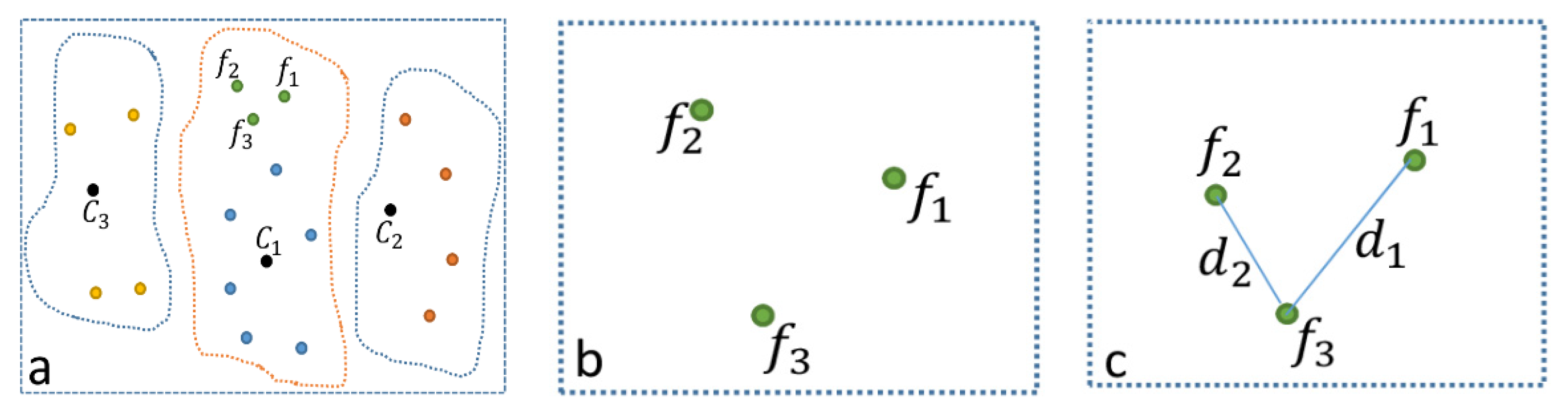$\Vert C_i-{\mu }_j\Vert$ is the Euclidean distance between the feature that is selected as the centroid ($C_i$) and other features (${\mu }_j$), which is used to find the features with longer distances from the extracted centroid of features, using Equation (8). The visualization of Equation (7) is shown in Figure 5. Then, it must be determined which neighboring segments are appropriate to accept the new features. Suppose $A=\left\{f_1,f_2,f_3,\dots \right\}$ is a set of features that are identified to be moved from one segment to other segments, as illustrated in Figure 5b. This set of features can be different types of features, as the area features are presented by their centroids and the lines are presented by their midpoints in the map segmentation step.

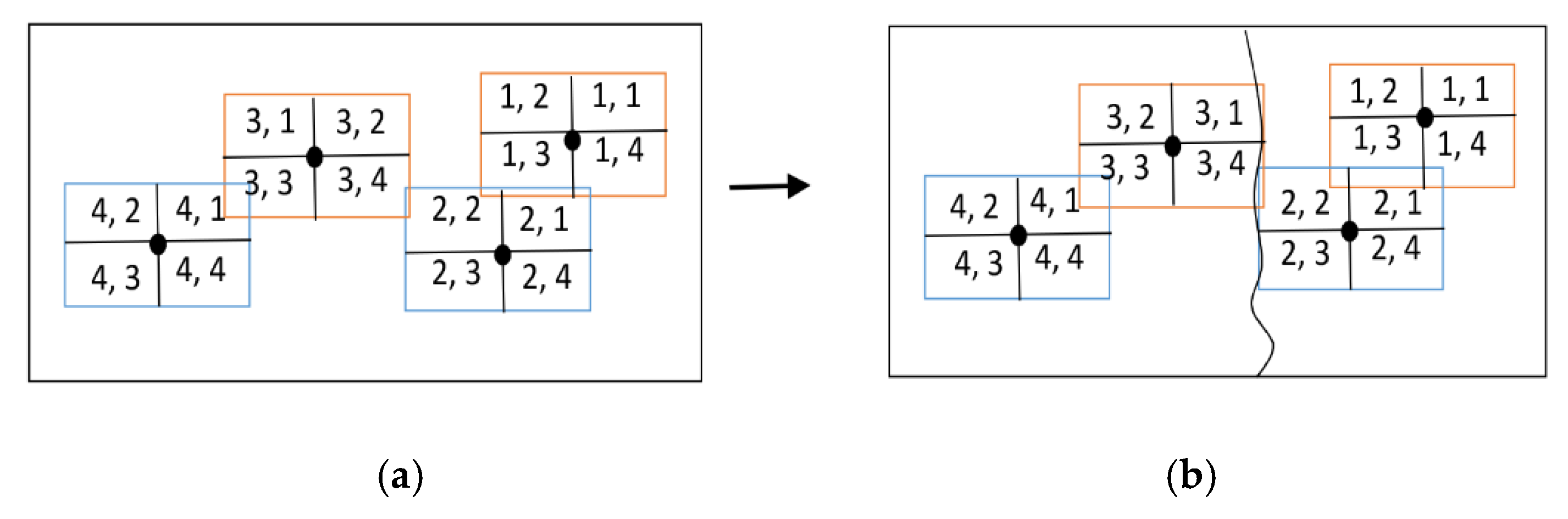
As shown in Figure 5, three subdomains exist; however, the segment with the centroid $C_1$ has more features in contrast to the two neighboring segments with the centroids $C_2$ and $C_3$. Some features have to be removed from the segment having the centroid $C_1$ and added to the neighboring segments accordingly. To adjust the distribution of the features, feature types are applied as the basis for devising in the adjusting phase. According to the cartographic standardization for feature labeling, the labels of line and area features are placed at various angles, horizontal, vertical, or along the direction of features. While the label of point features is often positioned horizontally, in this case, the probability of label conflict and label–feature conflicts increases during the process of feature label placement.

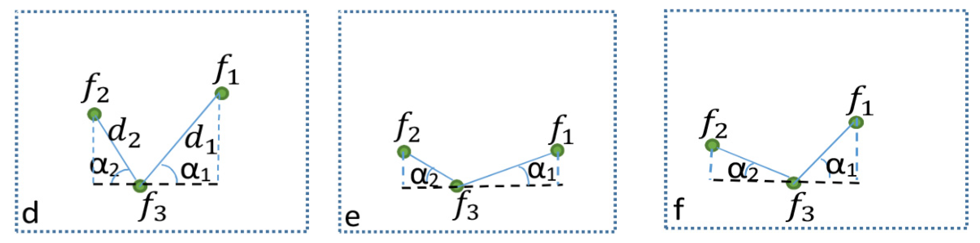
In Figure 5, assume the segment with the centroid $C_1$ violated Equation (6), and three features with indices $f_1,f_2, \mathrm{and} f_3$ are identified as the features to be removed from the segment with centroid $C_1$ and added to other segments based on Equation (8). To investigate the relationship between features in set $A=\left\{f_1,f_2,f_3,\dots \right\}$, five factors are considered: the distance between the features, the length of the label box for point feature, the height of the label box, the angle between features, and the buffer distance for the area and line features. Since the position of each label has an influence on the position of neighboring labels, the aforementioned factors are set to minimize the probability of label conflict. As shown in Figure 5a–f, features in set $A=\left\{f_1,f_2,f_3,\dots \right\}$, can have a variety of relationships.

$$d_{i,j}={{\displaystyle \sum }}_{i=1}^A\Vert x_i-{\mu }_j\Vert {}^2,{\forall }_{i<j}$$

(9)

$$if\{\hspace{1em}\begin{array}{c}{d}_{i,j}>L No dependecny \\ d_{i,j}<L Dependency of features in set A\end{array}$$

(10)

To study the relationship between features in set $A=\left\{f_1,f_2,f_3,\dots \right\}$, Equation (10) is formulized, where $L$ stands for the length of the label box. Note that the length of the label box is calculated according to the number of letters of labels. First, the dimension of each letter is measured based on the scale of the dataset and then multiplied by the number of letters; in this case, the label box generated is approximately the same size as the actual label. $d_{i,j}$ stands for the Euclidean distance between features $i \mathrm{and} j$. If the distance is less than the length of the label box of any of these two features, the features are assumed to be dependent; otherwise, they are assumed to be two independent features. Figure 5b shows that there is no possible relationship between features in set $A=\left\{f_1,f_2,f_3,\dots \right\}$, according to Equation (10); in such a case, each feature is added in different neighboring segments regardless of other features in set $A=\left\{f_1,f_2,f_3,\dots \right\}$. However, if there is any dependency between features in set $A$, as shown in Figure 5c, the feature with index $f_3$ has relationships with the two other features. On the other hand, none of the neighboring segments can accept all three features. The following equations are defined to identify which segment is appropriate to accept the features from set $A$ by assigning a weight value based on the condition of feature relationships:

$$\alpha >{45}^{°},\hspace{1em}{\phi }_1=\frac{h}{V_{i,j}},\hspace{1em}{\phi }_1^{\prime }=\frac{h}{V_{i,k}}$$

(11)

In Equation (11), if the angle $\alpha$ is greater than 45 degrees, the height of the label box and vertical distance are considered to assign weight values, as presented in Figure 5d. $h$ stands for the height of the label box; $V_{i,j} \mathrm{and} V_{i,k}$ are the vertical distances between features, as shown with blue dash line in Figure 5d; and ${\phi }_1 \mathrm{and} {\phi }_1^{\prime }$ are the weight values. If ${\phi }_1>{\phi }_1^{\prime }$, the features $i \mathrm{and} j$ are grouped as one category and can be moved in the same segment, and feature $k$ is assumed to be an independent feature and can be added to another segment.

$$\alpha \le {45}^{°},\hspace{1em}{\phi }_1=\frac{l}{H_{i,j}},\hspace{1em}{\phi }_1^{\prime }=\frac{l}{H_{i,k}}$$

(12)

In Equation (12), if the angle $\alpha$ is less than or equal to 45 degrees, the length of the label box for point features, buffer distance for the area and line features, and horizontal distances are considered to assign weight values. $l$ presents the length of label box for point feature and buffer distance for the line and area features; $H_{i,j} \mathrm{and} H_{j,k}$ are the horizontal distances between features, as shown with a black dash line in Figure 5e; and ${\phi }_1 \mathrm{and} {\phi }_1^{\prime }$ are the weight values. The greater weight value shows that the features must be grouped as one category and the lower weight value indicates that the dependency of features can be regarded as independent.

$${\alpha }_1>{45}^{°},\hspace{1em}{\alpha }_2\le {45}^{°},\hspace{1em}{\phi }_2=\frac{h}{V_{i,j}},\hspace{1em}{\phi }_2^{\prime }=\frac{l}{H_{i,k}}$$

(13)

Equation (13) describes the condition where the features in set $A=\left\{f_1,f_2,f_3,\dots \right\}$ are located in such a way that the angles $\alpha$ between them are less and greater than or equal to 45 degrees, as shown in Figure 5f. Therefore, these metrics are considered to assign weight values according to feature relationship to minimize the possibility of labels being positioned in conflict, which are the height ($h$) and length ($l$) of the label box and the horizontal ($H$) and vertical ($V$) distances between features. 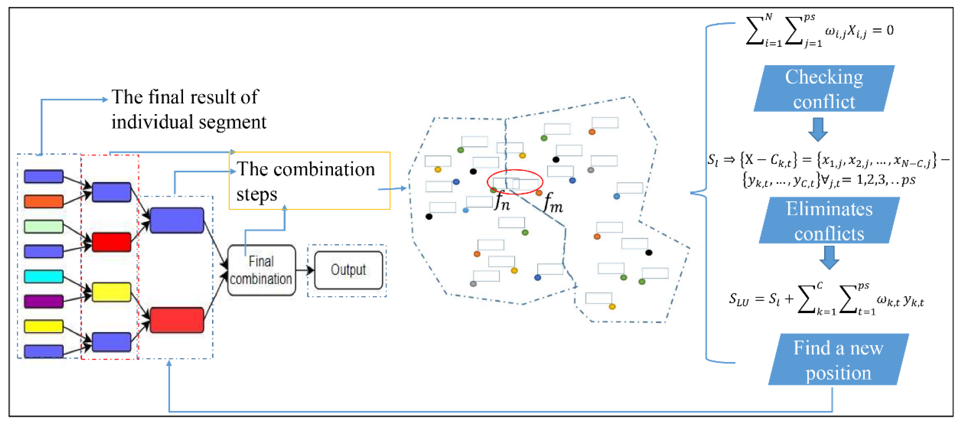Ultimately, based on the assigned weight values, the features in set $A$ will be categorized into different groups. Algorithm 1 presents the procedure of map segmentation.

Algorithm 1. Map segmentation

1: Specify the number of segments (n)

2: Count the number of features on the map (N)

3: Ideal feature division; I = N/n

4: maxv = I + 2; minv = I − 2

5: for i = 1…P do

6:    for j = 1…N do

7:       intersect i and j

8:    end for

9: end for

10: for i = 1…P do

11:     if the number of features (Ki) > maxv do  // Ki the number of features in segment (i)

12:       for L = 1…K do

13:          find the centroid of features (Ki) in segment (i)

14:        end for

15:        F = K − maxv // how many features are more than the defined range

16:        for f = 1…F do

17:           find the farthest features based on the centroid of segment (i)

18:        end for

19:        m = ${\displaystyle {\sum }_{}^{}f}$ // features need to be added to another segment

20:        check the dependency of features in set (A) based on Equations (10)–(13)

21:        for ii = 1…P do

22:           find the neighboring of segment (i)

23:           if Kii < max do  // if its features are less than the max value in this neighbor

24:              n = one possible segment to accept new features

25:           end if

26:        end for

27:        neighbors = ${\displaystyle {\sum }_{}^{}n}$ // All possible neighbors of segment (Ri)

28:        find the centroid features of each neighbor (C)

29:        for c = 1…C do

30:           measure the distance of each feature in set (A) to c

31:        add features from set (A) to the closest neighbor

32:        update the number of features of the neighbor segment that accepted from segment (i)

33:    end if

34: end for

3.2. Optimization Algorithm

The optimization algorithm of the proposed method is the hybrid of differential evolution (DDE) and genetic algorithm (GA) (see Section 2.2). This phase of the algorithm is composed of three phases: candidate position generation, finding the ideal solution from a large set of candidate position combinations, and the recombination result of each segment for the final output.

Candidate Position Generation and Quality Evaluation Function

In conformity with general rules of cartographic standardization in automatic label placement, several requirements for candidate position generation should be satisfied. The number of overlaps between labels and between label and feature must be minimized, and the orientation between labels and the corresponding feature must also be clear to maintain the highest probability of readability. Thereby, to realize MGFLP labels more effectively and with higher label quality, the quality evaluation function must consider esthetic properties, legibility, and clearness. Four fundamental quality factors are considered in the evaluation function of the proposed algorithm:

• Label–feature conflict factor;
• Label conflict factor;
• Label position priority factor;
• Ambiguity factor.

The input features are denoted as $N$, and the candidate positions are denoted as $ps$. So, based on four evaluation factors, the quality function is defined as follows:

$$Q\left(y\right)={\rho }_1\left(\gamma \right)+{\rho }_2\left(\gamma \right)$$

(14)

$${\rho }_1\left(\gamma \right)=\frac{F}{N}\ast 100$$

(15)

$${{\displaystyle \sum }}_{i=1}^N{{\displaystyle \sum }}_{j=1}^{ps}{w}_{i,j}{x}_{i,j}=0$$

(16)

Equation (14) is the general formula for quality function; ${\rho }_1\left(\gamma \right)$ presents the percentage of features being labeled, and ${\rho }_2\left(\gamma \right)$ presents the sum of scores of all four quality metrics. In Equation (15), $F$ is the total number of features that are labeled and $N$ is the total number of input features. Equation (16) ensures that the features are labeled. If the value is zero, the feature is labeled; otherwise, the feature is not labeled.

$${\rho }_2\left(\gamma \right)={{\displaystyle \sum }}_{i=1}^n\left(\left[{{\displaystyle \sum }}_{i=1}^N{{\displaystyle \sum }}_{j=1}^{ps}\left(F_{i,j}^{Over}+F_{i,j}^{Pos}+F_{i,j}^{Amb}\right)\right]\right)$$

(17)

In Equation (17), $n$ is the number of segments, $F_{i,j}^{Over}$ presents label conflict and label–feature conflict, $F_{i,j}^{Pos}$ presents label position priority, and $F_{i,j}^{Amb}$ presents the ambiguity factor. Our objective is to minimize the value of ${\rho }_2\left(\gamma \right)$ function to ensure that the optimal positions are quantitatively evaluated. In this study, the considered quality factors are briefly explained; however, they are discussed in detail in [32].

$$F_{i,j}^{Over}=\{ \begin{array}{c}\{\begin{array}{c}{\omega }_1=0 No label-label conflict \\ {\omega }_1>0 Label-label conflict\hspace{1em}\end{array}\\ \{\begin{array}{c}{\omega }_2=0 No label-feature conflict\\ {\omega }_2>0 Label-feature conflict\end{array}\end{array}$$

(18)

Equation (18) illustrates label–label and label–feature conflicts, where zero shows no conflict occurring and greater than zero presents conflict. From the perspective of feature importance, the weight of label conflict with point feature is set greater compared to the weights of label conflict with line and area features, as it can be observed in the finding that no labels are in conflict with point features.

Equations (19) and (20) present the label position priority, and it is only considered for point and area features. Equation (19) is defined for label position priority of point features, where all positions in the first quadrant have the highest priority and its priority declines anti-clockwise, which is presented by angle $\beta$. Equation (20) is defined for label position priority of area features, where $\ell$ is the distance from the center of the label box to the midpoint of the approximate skeleton line of the area feature. ${\ell }_{min} and {\ell }_{max}$ present the minimum and maximum distances of all candidate positions to the feature skeleton line, respectively. The smaller the value $F_{i,j}^{Pos}$ is, the higher the label position priority is.

$$F_{i,j}^{Pos}=\{\begin{array}{c}\omega =0.25,\hspace{1em}\hspace{1em}\beta \in \left[0^{°},{90}^{°}\right)\\ \hspace{1em}\omega =0.5,\hspace{1em} \beta \in \left[{90}^{°},{180}^{°}\right)\hspace{1em}\\ \omega =0.75,\hspace{1em}\hspace{1em}\beta \in \left[{180}^{°},{270}^{°}\right)\\ \omega =1.0,\hspace{1em}\beta \in \left[{270}^{°},{360}^{°}\right)\end{array}$$

(19)

$$F_{i,j}^{Pos}=\frac{\ell -{\ell }_{min}}{{\ell }_{max}-{\ell }_{min}}, {\ell }_{min}<\ell <{\ell }_{max}$$

(20)

Equation (21) measures the ambiguity of the label and its corresponding feature; this quality factor was only taken into account for line features, and it calculates the distance of the selected label to the midpoint of the corresponding line feature. $D$ is the distance of the center of the label box to the line feature, and $D_{min} \mathrm{and} D_{max}$ are the minimum and maximum distances of all candidate positions to the corresponding feature, respectively.

$$F_{i,j}^{Amb}=\frac{D-D_{min}}{D_{max}-D_{min}}, D_{min}\le D\le D_{max}$$

(21)

Algorithm 2 reports that the algorithm starts with the generation of candidate positions for the given features. When the generation of candidate positions is completed, the optimization phase begins with the selection of random initial populations, and then the fitness values of these populations are calculated and sorted. The selection of the population for each iteration is being exerted 30% by the DDE algorithm and 70% by the GA based on the fitness value. For terminating the iteration cycle, two conditions are set. First, if the fitness value of the obtained result is less than a threshold value, the loop iteration is terminated; otherwise, continue. Second, an iteration number is set; the optimization phase terminates after this number of iterations if the fitness value does not meet the first condition.

Algorithm 2. Optimization algorithm

1: Generating candidate Positions

2: set the parameters: mutation and crossover probability, termination (num- gen (t))

3: initialize the population with pop-size $\left(p\right)$

4: while termination is note satisfied (iter < $z$) do

5:    for the genotype of each individual $g_i\left(z\right)\in p\left(t\right)$ do

6:       evaluate the fitness of $g_i\left(z\right)$

7:    end for

8:    sorting the fitness values

9:    if fitness $g_i\left(z\right)$ < threshold value do

10:       break

11:    end if

12:    else do

13:      if the value of $g_i\left(z\right)<g_{i-1}\left(z\right)$ do

14:          replace new genotypes

15:      end if

16:      $P_1^{\prime }$ = 50% of best P(i)

17:       for genotype (int(30% * pop-size)) do

18:          $P_1^{″}$ = chose random genotype of P(i)

19:          $P_1$ += crossover ($P_1^{″}$ and $P_1^{\prime }$)  // In total 70% of genotype generated by GA

20:       end for

21:       while $P_1$< pop-size do // 30% of genotype generated by DDE

22:                     $P_1$+= [random selection of the best Pi]

23:       end while

24:       mutation operation

25:    end else

26:    iter += iter

27: end  while

3.3. Removing Label Conflict after Recombining the Result of Subdomain

To investigate label conflicts after recombining the result of each individual segment, an additional supplementary step is added in the proposed algorithm. Once the labeling process is completed in the second phase of the algorithm in each subdomain, the steps of recombination are implemented according to the two neighboring subdomains. First, the results of two neighbor subdomains are combined, and the rest of them wait until the combination of the two neighboring subdomains is completed; then, the two combined results recombine in the next step with the result of another subdomain. These procedures continue until all subdomains are combined. Figure 6 illustrates the steps of recombining the results of all segments after the optimization phase.

As it can be seen in Figure 6, on the left side of the figure, small colored boxes represent the final result of each subdomain, and the combination of results is carried out step by step as two neighboring segments. However, after the recombination phase, the presumption of label conflict is potentially high, especially near the boundary of segments, which negatively affects label placement quality, as shown by $f_n$ and $f_m$ in Figure 6. Therefore, after recombination of each two neighboring segments, the following steps (see Equations (22)–(25)) are defined to be implemented in order to eliminate or minimize the number of label conflicts:

$${{\displaystyle \sum }}_{i=1}^N{{\displaystyle \sum }}_{j=1}^{ps}{\omega }_{i,j}{X}_{i,j}=0$$

(22)

$$S_l\Rightarrow \left\{\mathrm{X}\right\}=\left\{x_{1,j},x_{2,j},\dots ,x_{N,j}\right\}{\forall }_j=1,2,3,\dots ps$$

(23)

$$S_l\Rightarrow \left\{X-C_{k,t}\right\}=\left\{x_{1,j},x_{2,j},\dots ,x_{N-C,j}\right\}-\left\{y_{k,t},\dots ,y_{C,t}\right\}{\forall }_{j,t}=1,2,3,\dots ps$$

(24)

Equation (22) ensures that label conflict does not occur if the value is zero. Otherwise, label conflict occurs after the recombination of the results of two neighboring segments. ${\omega }_{i,j}$ is the weight value, and $X_{i,j}\in \left[0,1\right]$ is a variable. $C_{k,t}$ denotes a set of features with labels that are in conflict after recombination with the label $j$ of feature $i$. In Equation (23), $S_l$ is the recombination of label positions of two segments. Equation (24) shows that $C_{k,t}$ will be removed from the label list ($S_l$). $S_l$ presents the positions of labels, and $y_{k,t}$ represents the position $t$ of feature $k$ having a conflict with another label, and it necessitates the identification of an alternative position that can remove the label conflict. The final equation is formulated as follows:

$$S_{LU}=S_l+{{\displaystyle \sum }}_{k=1}^C{{\displaystyle \sum }}_{t=1}^{ps}{\omega }_{k,t}{y}_{k,t}\hspace{1em}{\forall }_t=1,2,3,\dots ps$$

(25)

where $S_{LU}$ is the label list updated with new label positions, and $S_l$ now presents the label list after removing $C_{k,t}$. This step is continued in each step of recombination until the result of all segments is combined. The following steps show the selection of new positions for label conflict in each stage of recombination:

• (i) For i = 0 to the length of $C_{k,t}$ do:

• Find all combinations of $C_{k,t}$ with all positions of feature which had overlap;
• Check if there is any overlap between new generated combinations;
• Select the combination with no overlap;
• If all new combinations are in overlap, select the one with the smallest number of overlaps;
• End.

4. Computational Results

The experiments were implemented on a machine with Intel Core i5-8265U CPU @1.60 GHz 1.8 GHz, running in Windows 10 Professional × 64 with 16.00 GB RAM installed. The code was written in Python language, using Pycharm framework based on Arcpy template using ArcGIS Pro. Message Passing Interface (MPI) library was used for parallel processing [44,45].

To evaluate the robustness and stability of the proposed algorithm (Parallel-MS), the experiments were implemented on three different real-world datasets, each containing multiple geographical features, as shown in

Table 1. Three real-world datasets with multiple geographical features.

Dataset	Area	Line	Point	Total	Scale	Location
First	39	17	15	71	1:4,000,000	Washington, USA
Second	0	10	56	66	1:1500	Part of Chicago, USA
Third	88	20	36	144	1:2,800,000	Ohio, USA

. The experimental parameters were set as follows: the number of iterations was set to 10,000; crossover rate and mutation rate were 0.5 and 0.01, respectively; and 24 candidate positions were generated for each feature in two degrees of freedom space [32]. The obtained results are compared with the DDEGA algorithm, DDEGA-NM algorithm, and Maplex Label Engine to evaluate the applicability of the Parallel-MS.

4.1. Investigating the Performance of the Algorithm Based on Different Numbers of Segmentations

Map segmentation allows us to decompose the problem of map labeling into subtasks that can be managed concurrently. The aim of this experiment is to examine how the number of segments affects label placement quality and the acceleration performance of the algorithm. Five groups of experiments were implemented by varying the number of segments from 2 to 10 with an increment of 2. Each experiment ran five times, and then the best results after five runs for each group of the experiment were selected for comparison, as shown in

Table 2. Applying different numbers of segmentations on the first dataset.

Segmentation	The Number of Label–Feature Conflicts				Label Conflict	Score	Time (min)
	Point	Line	Area	Total
2	1	4	12	17	0	4.083	182.47
4	0	3	12	15	0	3.035	92.26
6	1	2	8	11	0	2.817	50.27
8	0	2	8	11	0	1.856	20.39
10	0	2	10	12	1	6.481	15.15

and

Table 3. Applying different numbers of segmentations on the second dataset.

Segmentation	The Number of Label–Feature Conflicts			Label Conflict	Score	Time (min)
	Point	Line	Total
2	4	4	8	0	2.981	164.32
4	3	2	5	0	2.870	80.54
6	4	0	4	0	2.083	39.27
8	3	0	4	0	1.784	16.03
10	2	1	3	1	5.552	11.51

. The results were analyzed based on four metrics, namely the number of label conflicts, label–feature conflicts, score value, and computation time.

The results of the first and second datasets are shown in Table 2 and Table 3, respectively. Table 2 and Table 3 show that the computational complexity of the algorithm is reduced as the number of segments increases, enabling the algorithm to find the ideal solution instinctively. However, the number of segments is not infinite; thus, a suitable number must be set for segmentation. Otherwise, the probability of label conflict increases after the recombination of the result of each segment. This occurs when some labels are positioned near the boundary of segmentation, and the position of those labels can cause label conflict, particularly in feature-intensive areas. Due to the dependency of labels of features, the position of one label can affect neighboring labels, which leads to the labels being placed in conflict. As both tables present, label conflict occurred when the number of segments was set to 10. Therefore, increasing the number of segments leads to improvement in the computational performance of the algorithm; however, the score value is negatively influenced after 10 segments, indicating that the number of segments is not infinite. Hence, it is fundamentally important to select an appropriate number for segmentation, and its potential effect should be necessarily considered and evaluated.

4.2. Performance Analysis of Parallel Version vs. Serial Version of Map Segmentation with Different Segments

To examine how the concept of map segmentation can reduce the computational complexity, the experimental results were compared based on serial and parallel versions after applying the map segmentation. In the serial version of the algorithm, one CPU was employed to complete the procedure of automatic label placement of each segment in turn. The running times of the parallel version and serial version of the algorithm are shown in Figure 7a. As the figure shows, the execution time of the algorithm is significantly reduced when the number of segments is increased in both versions of the algorithm. Applying parallel computation significantly reduced the overall computation time. There was a 239 min reduction in computational time when the number of segments increased from 2 to 10 in the serial version and a 159 min reduction in the parallel version of the first dataset. On the second dataset, the same performance was achieved, 221 and 153.07 min in serial and parallel versions, respectively. Furthermore, the amount of speed and the ratio of speedup were measured to analyze the performance of the algorithm as well, as shown in Figure 7b. The speedup metric evaluates the amount of speed gained by increasing the number of segments, and the ratio of speedup describes the amount of speed that each CPU can achieve. The results illustrate that decomposing a complex problem into subproblems reduces the computation steps and further leads the algorithm to identify the ideal solution in a small iteration cycle.

Apart from the aforementioned factors, the performance of the algorithm has been extensively analyzed in terms of label position accuracy based on the score value of the quality function. The aim is to minimize the value of the quality function in order to retrieve a solution with high quality (see Section 3.2). This experiment includes two metrics, the score values of serial and parallel versions of all three datasets. The figure depicts that the score values are reduced in both versions of the algorithm in response to the increase in segments. However, the score values increased when the number of segments was set to 10, as shown in Figure 7c, which is potentially caused by label conflict after the recombination of individual segments. Thus, 8 was selected as the best number of segments for the current datasets according to the experimental analysis. Furthermore, Figure 7d illustrates the speed of the convergence of score values during the iteration cycle on one dataset. As it can be observed, the higher the number of segments is, the lower the score value is in each iteration. Values along the y-axis show the score values and values along the x-axis represent the number of iterations. At the starting of the iteration, the score value of the algorithm with two segments is the highest; in contrast, 10 segments have the lowest score value. The score has a dramatic decreasing trend from the first iteration to 1000 iterations, while between 1000 and 9000 iterations, the score values show a gradual decline; on the contrary, from 9000 to 10,000, all segments maintained the same value apart from 10 segments, which showed a slight rise. Although 10 segments initially had the lowest score, they outraced all segments at the end of the iteration due to the combination of the result of 10 segments as final output, which caused one label–label conflict.

Therefore, this certifies that identifying the ideal solution for map labeling is better facilitated by decomposing the problem of label placement into subproblems. To sum up, the figures demonstrate that applying map segmentation enables the algorithm to reduce the computational complexity of multiple geographical feature label placement; even without parallel computation, the execution time of the algorithm is dramatically decreased. Additionally, the utilization of parallel computing sped up the algorithm linearly. Whereas the computational cost is influenced by increasing the number of features, the advantages of map segmentation and parallel processing become increasingly obvious in large-scale solutions, as they substantially reduce the computational complexity and obtain a solution with high quality.

4.3. Comparison Analysis of the Proposed Algorithm with Previous Studies

To quantitatively evaluate the practicality and effectiveness of the Parallel-MS algorithm, the obtained results are compared with previous studies. It should be noted that the basis of candidate position generation of the developed algorithm is the DDEGA-NM algorithm. Three experimental datasets were selected based on large and small scales in order to study the practical application of the Parallel-MS algorithm, and then the results were analyzed extensively in comparison with previous approaches. To begin with, the final result of the first dataset that was obtained by the DDEGA-NM algorithm is shown in Figure 8, and the result achieved by Parallel-MS algorithm is shown in Figure 9. Figure 8 shows that despite having more overlap, many labels of area features are positioned near the boundary of the area feature, which can cause more ambiguity for the readers, and some labels are placed closely together additionally. Moreover, two point features are covered by their labels. On the contrary, as Figure 9 shows, the result of label placement of the Parallel-MS algorithm is more precise, almost all features labels are positioned at the center of the area features, and no labels have conflicts with point features. Furthermore, the number of label–feature conflicts decreased from 23 to 12, and labels are placed at the most desirable position. Following, the result of the second dataset obtained by the DDEGA-NM algorithm is shown in Figure 10, and the Parallel-MS result is presented in Figure 11. By the same token, some labels are positioned far from their corresponding features, and they even are closer to the other features (see Figure 10), namely “Windy City Diamonds” and “Pizanos Pizza & Pasta”. Those labels can cause misunderstanding for readers. In addition, three labels have conflicts with line features, and some labels of point features cover a small portion of their features; apart from this, one line feature is left without a label. The results of the proposed algorithm, conversely, in both parallel and serial versions (Serial-MS) show that most of those issues are solved, labels are placed near their related features, and the number of labels that covered their corresponding features is decreased considerably, as shown in Figure 11. Only one label is in conflict with the line feature. The results of Parallel-MS were also compared with other algorithms, and the statistical results are shown in

Table 4. Comparison of the proposed algorithm with previous algorithms on the first dataset.

Algorithms	The Number of Label–Feature Conflicts				Label Conflict	Score	(%)	Time (min)
	Point	Line	Area	Total
GA	0	9	31	40	0	//	100	//
DDE	0	10	30	40	0	//	98.485	//
DDEGA	0	6	27	33	0	//	100	3060
Maplex	0	8	29	37	0	//	100	//
DDEGA-NM	2	7	13	22	0	8.143	100	2166
Serial-MS	0	3	8	12	0	2.125	100	225
Parallel-MS	0	2	9	12	0	1.913	100	20

,

Table 5. Comparison of the proposed algorithm with previous algorithms on the second dataset.

Algorithms	The Number of Label–Feature Conflicts			Label Conflict	Score	(%)	Time (min)
	Point	Line	Total
DDEGA	5	3	8	0	//	100	2887
DDEGA-NM	4	4	8	0	3.254	98.485	2345
Serial-MS	2	0	2	0	1.643	100	214
Parallel-MS	3	0	3	0	1.784	100	16

and

Table 6. Comparison of the proposed algorithm with Maplex Label Engine on the third dataset.

Algorithms	The Number of Label–Feature Conflicts				Label Conflict	(%)	Time (min)
	Point	Line	Area	Total
Maplex	16	14	35	65	14	90.277	//
Serial-MS	2	11	15	28	4	97.222	486
Parallel-MS	3	12	14	29	6	95.833	45

.

Table 5 presents that the comparison begins not only with the DDEGA-NM algorithm but also with other algorithms by examining the performance of each algorithm on the same datasets. GA stands for the result of genetic algorithm, DDE represents discrete differential evolution result, and DDEGA is the hybrid of GA and DDE evolutionary algorithms. The Maplex Label Engine optimization was also implemented, in addition to the mentioned algorithms. The “%” column illustrates the percentage of features being labeled in the final result. In addition, in both tables, some rows are filled with the “//” symbol due to the lack of score value since those algorithms used different quality functions. First and foremost, the DDEGA algorithm iterated 300 iterations in 3060 min with 33 label–feature conflicts, and the DDEGA-NM algorithm iterated 10,000 iterations in 2166 min and gained the result with 22 label–feature conflicts (see Table 4). However, on the same dataset, the serial version of the proposed algorithm iterated 10,000 iterations in 225 minutes, and the parallel version finished the same number of iterations in 20 min with 12 label–feature conflicts.

Compared to previous approaches, the obtained results are much better relative to the results of other methods. Following, the number of label–feature conflicts and label conflicts in GA and DDE is 40, and Maplex achieved a result with 37 label–feature conflicts. The comparison on the second dataset was only implemented between the DDEGA algorithm, DDEGA-NM algorithm, and the proposed algorithm, and the results are presented in Table 4. Similar to the first dataset, the number of iterations was set to 300 for the DDEGA algorithm, the algorithm iterated in 2887 min, and eight labels conflicted with the features. The DDEGA-NM algorithm iterated 10,000 iterations in 2354 min with eight label–feature conflicts, which accelerated the execution time dramatically. The serial and parallel versions of the proposed algorithm, on the other hand, iterated 10,000 iterations in 214 and 16.03 min, respectively; two labels are in conflict with features in the serial version and three labels are in conflict with features in the parallel version. The obtained result of the third dataset by the proposed algorithm is presented in Figure 12, and its statistical analysis is reported in Table 6. Figure 13 is the result achieved by Maplex Label Engine, which has 65 label–feature conflicts. However, the numbers of label–feature conflicts in our approach are 28 and 29 in serial and parallel versions, respectively. Noting that the number of iterations was set to 10,000 for all experiments, the running time of the serial version of our algorithm is 486 min which declined to just 45 min in the parallel version of the algorithm. Among 144 features, 14 features were left without labels using Maplex Label Engine, and 4 and 6 features were left without labels in our serial and parallel algorithms, respectively.

Therefore, the tables report that the previous approaches, including Maplex Label Engine, achieved a result in which the number of label–feature conflicts is much higher compared to the parallel and serial versions of map segmentation, the quality of label positioning is much lower compared to the standard labeling quality, and the computational time of other algorithms is crucially longer. Consequently, the proposed algorithm is well improved to solve the problem of MGFLP. On the whole, map segmentation strengthens the algorithm to explore most of the search solutions intuitively. Moreover, taking the approach of parallel computing sped up the algorithm significantly; it gained superlinear speedup compared to the mentioned algorithms.

5. Discussion

Experimental results demonstrate the usability and scalability of the proposed algorithm and substantially improved geographic feature label placement quality in both of the following aspects: (1) reduced the computational time of the problem by decomposing into smaller scale; (2) most of the labels are positioned at their desired positions. However, all pre-existing studies used the serial version of the algorithm to address the problem of automatic label placement. In this research, the authors extended the procedure of label placement beyond the traditional approaches by considering the concept of map segmentation and the utilization of parallel processing. To illustrate the notion of map segmentation (see Figure 4 in Section 3), four candidate positions are defined for each feature; without map segmentation, $4^4$ combinations are required to check all the possible candidate positions combinations, despite there being no direct dependency between features (1, 4), (1, 3), and (2, 4). In contrast, if the map is segmented into two subdomains, as shown in Figure 4b, the number of steps that check all the solutions for both subdomains is reduced from $4^4$= 256 to $4^2+4^2=$ 32 combinations. Thus, segmenting the map into several subdomains enables the algorithms to refrain from taking nonessential computational steps, which causes the algorithm to avoid being trapped in local minima and to not iterate through repetitive solutions, as well as reducing the computational time. These are the fundamental components while designing a comprehensive algorithm to cope with a combinatorial optimization problem. To substantially accelerate the speed of the algorithm, each segment is designated on a discrete CPU to facilitate the algorithm to run concurrently, which gained superlinear speedup compared to the previous works, as shown by the results presented in Table 4, Table 5 and Table 6.

Further, each feature label has 24 candidate positions in the current study; thus, the total number of generated solutions is $N^{24}$, where $N$ is the number of features. Identifying the ideal solution from such a large number of solutions is extremely difficult as one search domain within a reasonable time span and is a fundamental challenge in cartography. However, if the search domain is decomposed into several independent subdomains, the solution can be identified more intuitively with less computational time. While decomposing the problem of map labeling, a key challenge has arisen: label conflict after the recombination of subdomain results. To cope with the mentioned issue, an additional supplementary step is added to the algorithm that investigates the potential label conflict after each step of results recombination and identifies alternative positions for the labels with conflict. Note that all label conflicts are eliminated in all experimental datasets. Conversely, as the results demonstrate, there are still some label–feature conflicts, as shown in Figure 9, namely Seattle, Bremerton, Tacoma, Olympia, Aberdeen, and line I182. The elimination of these conflicts is almost impossible even manually due to the lack of enough space for labels of those features because of intense feature density, and there is no free space around the features to place the labels without label–feature conflict. As the third dataset illustrates, the number of features is 144, which also includes multiple geographical features, and the introduced approach obtained a good result. This result was not compared with DDEGA and DDEGA-NM algorithms, because they would take several days to finish the iteration cycle of 10,000.

There exists a pronounced trend to identify the ideal solution with HPC if a proper number of segments is chosen for the map. Several experiments were implemented to find a proper number for segmentation. As shown in Table 2 and Table 3, while the number of segmentation increases, the computational time decreases in serial and parallel versions of the algorithm because the number of computational steps is reduced and the algorithm seeks the solution concurrently. In addition, the probability of finding the new solution in each iteration cycle is higher compared to a complex problem without decomposing, as presented in Table 2 and Table 3. Therefore, special attention should be paid to the limited number of segments, as exceeding this limitation might cause more label conflicts in the final result, which are costly to eliminate and negatively influence the algorithm performance.

6. Conclusions

Multiple geographical feature label placement is a combinatorial optimization problem. Despite a long history of research to solve this problem, there is not any approach to verify the optimal solution to this problem. Several heuristics and metaheuristics have been introduced, and some considered the notion of conflict graph to address the problem of feature label placement. However, most of the heuristic approaches that were applied struggle with serious challenges, the algorithms become trapped in local minima, and the computational time is crucially long.

This paper has presented a novel parallel algorithm with the concept of map segmentation to address the automatic label placement problem. To begin with, map segmentation enables the algorithm to decompose the problem of label placement into a smaller scale for coping with the computational intensity of labeling and identifying the ideal solution intuitively; it also improves the scalability and optimizes the performance of the algorithm. Next, parallel computing is applied to handle each segment concurrently on a separate processor to exploit the computational advantages of parallel processing. To generate appropriate candidate positions around points and line features and around or within area features, four quality factors are considered: label conflict, label–feature conflict, label ambiguity, and label position priority. For verifying the efficiency of the proposed algorithm, three datasets were selected for the experimental analysis, and each contained multiple geographical features. The experimental results demonstrate that 14.084% and 7.576% improvements have been achieved in terms of the number of label–feature conflicts for the first and second datasets, respectively, compared to the most recent study [32]. Moreover, 108.3% and 146.288% improvements have been achieved in computational time for the first and second datasets, respectively. By the same token, the number of label–feature conflicts decreased from 65 to 29 compared to Maplex Label Engine. Thus, by adopting the presented algorithm, the cartographers can consider large-scale data for feature label placement.

Furthermore, it must be noted that although the proposed algorithm improved the quality of label placement and accelerated the speed of labeling, it is important to address several limitations in future studies. First and foremost, further study is needed on the application of the proposed algorithm on maps with a high degree of feature density. Following, there is a need for more research on finding a correlation between the number of segments and the input features automatically. In addition, adding more quality metrics in the quality evaluation function for candidate generation can improve the procedure of candidate generation, which decreases the probability of label conflict and label–feature conflict, likewise helping the algorithm to find a better combination of solutions in fewer iterations.

References

1. Liao, H.; Wang, X.; Dong, W.; Meng, L. Measuring the influence of map label density on perceived complexity: A user study using eye tracking. Cartogr. Geogr. Inf. Sci. 2018, 46, 210–227. [Google Scholar] [CrossRef]
2. Ding, Y.; Jiang, N.; Wu, C.; Zhou, X. A two-phase algorithm for point-feature cartographic label placement. Earth Sci. Inform. 2017, 11, 183–203. [Google Scholar] [CrossRef]
3. Yoeli, P. The Logic of Automated Map Lettering. Cartogr. J. 1972, 9, 99–108. [Google Scholar] [CrossRef]
4. Imhof, E. Positioning names on maps. Am. Cartogr. 1975, 2, 128–144. [Google Scholar] [CrossRef]
5. Lhuillier, A.; van Garderen, M.; Weiskopf, D. Density-based label placement. Vis. Comput. 2019, 35, 1041–1052. [Google Scholar] [CrossRef]
6. Morrison, J. Computer Technology and Cartographic Change; Johns Hopkins University Press: New York, NY, USA, 1980. [Google Scholar]
7. Christensen, J.; Marks, J.; Shieber, S. An empirical study of algorithms for point-feature label placement. Acm Trans. Graph. 1995, 14, 203–232. [Google Scholar] [CrossRef] [Green Version]
8. Formann, M.; Wagner, F. A packing problem with applications to lettering of maps. In Proceedings of the Seventh Annual Symposium on Computational Geometry, North Conway, NH, USA, 10–12 June 1991; pp. 281–288. [Google Scholar]
9. Marks, J.; Shieber, S.M. The Computational Complexity of Cartographic Label Placement; Technical Report TR-05-91; Harvard University: Cambridge, MA, USA, 1991. [Google Scholar]
10. Chirié, F. Automated Name Placement With High Cartographic Quality: City Street Maps. Cartogr. Geogr. Inf. Sci. 2000, 27, 101–110. [Google Scholar] [CrossRef]
11. Guerine, M.; Rosseti, I.; Plastino, A. A hybrid data mining heuristic to solve the point-feature cartographic label placement problem. Int. Trans. Oper. Res. 2019, 27, 1189–1209. [Google Scholar] [CrossRef]
12. Zoraster, S. The solution of large 0–1 integer programming problems encountered in automated cartography. Oper. Res. 1990, 38, 752–759. [Google Scholar] [CrossRef] [Green Version]
13. Christensen, J.; Shieber, S.M.; Marks, J. Placing Text Labels on Maps and Diagrams; Graphics Gems IV; Academic Press: Cambridge, MA, USA, 1994. [Google Scholar]
14. Strijk, T.; Verweij, A.; Aardal, K. Algorithms for Maximum Independent Set Applied to Map Labelling; Technical Report UU-CS-2000-22; Department of Information and Computing Sciences, Utrecht University: Utrecht, The Netherlands, 2000. [Google Scholar]
15. Marín, A.; Pelegrín, M. Towards unambiguous map labeling—Integer programming approach and heuristic algorithm. Expert Syst. Appl. 2018, 98, 221–241. [Google Scholar] [CrossRef]
16. Lei, Y.; Ai, T.; Zhang, X.; Li, J. A parallel annotation placement method for dense point of interest labels using hexagonal grid. Cartogr. Geogr. Inf. Sci. 2020, 48, 95–104. [Google Scholar] [CrossRef]
17. Ribeiro, G.M.; Lorena, L.A.N. Lagrangean relaxation with clusters for point-feature cartographic label placement problems. Comput. Oper. Res. 2008, 35, 2129–2140. [Google Scholar] [CrossRef]
18. Gomes, S.P.; Ribeiro, G.M.; Lorena, L. Dispersion for the point-feature cartographic label placement problem. Expert Syst. Appl. 2013, 40, 5878–5883. [Google Scholar] [CrossRef]
19. Rylov, M.A.; Reimer, A.W. A Comprehensive Multi-criteria Model for High Cartographic Quality Point-Feature Label Placement. Cartogr. Int. J. Geogr. Inf. Geovis. 2014, 49, 52–68. [Google Scholar] [CrossRef]
20. Haunert, J.-H.; Wolff, A. Beyond Maximum Independent Set: An Extended Integer Programming Formulation for Point Labeling. ISPRS Int. J. Geo-Inf. 2017, 6, 342. [Google Scholar] [CrossRef] [Green Version]
21. Li, L.; Zhang, H.; Zhu, H.; Kuai, X.; Hu, W. A labeling model based on the region of movability for point-feature label placement. ISPRS Int. J. Geo-Inf. 2016, 5, 159. [Google Scholar] [CrossRef] [Green Version]
22. Niedermann, B.; Haunert, J.-H. An Algorithmic Framework for Labeling Network Maps. Algorithmica 2018, 80, 1493–1533. [Google Scholar] [CrossRef] [Green Version]
23. Gemsa, A.; Niedermann, B.; Nöllenburg, M. Placing Labels in Road Maps: Algorithms and Complexity. Algorithmica 2020, 82, 1881–1908. [Google Scholar] [CrossRef] [Green Version]
24. Wolff, A.; Knipping, L.; van Kreveld, M.; Strijk, T.; Agarwal, P.K. A simple and efficient algorithm for high-quality line labeling. In GIS and GeoComputation; CRC Press: Boca Raton, FL, USA, 2001. [Google Scholar]
25. Sun, S.; Zhao, H.; Fang, J.; Cheng, Z.; Zhao, Y. A pratical method for line labeling. In Proceedings of the 2010 18th International Conference on Geoinformatics, GIScience in Change, Peking University, Beijin, China, 18–20 June 2010; pp. 1–6. [Google Scholar]
26. Wu, C.; Ding, Y.; Zhou, X.; Lu, G. A grid algorithm suitable for line and area feature label placement. Environ. Earth Sci. 2016, 75, 1368. [Google Scholar] [CrossRef]
27. Barrault, M.J.C. A methodology for placement and evaluation of area map labels. Comput. Environ. Urban Syst. 2001, 25, 33–52. [Google Scholar] [CrossRef]
28. Rylov, M.; Reimer, A. A practical algorithm for the external annotation of area features. Cartogr. J. 2017, 54, 61–76. [Google Scholar] [CrossRef]
29. Li, Y.; Sakamoto, M.; Shinohara, T.; Satoh, T. Automatic Label Placement of Area-Features Using Deep Learning. ISPRS—Int. Arch. Photogramm. Remote Sens. Spat. Inf. Sci. 2020, 43, 117–122. [Google Scholar] [CrossRef]
30. Pokonieczny, K.; Borkowska, S. Using artificial neural network for labelling polygon features in topographic maps. GeoScape 2019, 13, 125–131. [Google Scholar] [CrossRef] [Green Version]
31. Lu, F.; Deng, J.; Li, S.; Deng, H. A Hybrid of Differential Evolution and Genetic Algorithm for the Multiple Geographical Feature Label Placement Problem. ISPRS Int. J. Geo-Inf. 2019, 8, 237. [Google Scholar] [CrossRef] [Green Version]
32. Deng, J.; Zhiyong, G.; Mohammad Naser, L. Multiple Geographical Feature Label Placement Based on Multiple Candidate Positions in Two degrees of Freedom Space. IEEE Access 2021, 9, 144085–144105. [Google Scholar] [CrossRef]
33. John, H.H. Adaptation in Natural and Artificial Systems. U. Mich. Press 1975, 38, 15. [Google Scholar] [CrossRef]
34. Ahmad, S.; Fatma Farooqi, Y.; Rai, A. Coloring Vertices of a Graph Using Parallel Genetic Algorithm; Springer: Cham, Switzerland, 2020; pp. 765–769. [Google Scholar] [CrossRef]
35. Katoch, S.; Chauhan, S.S.; Kumar, V. A review on genetic algorithm: Past, present, and future. Multimed Tools Appl. 2020, 8091–8126. [Google Scholar] [CrossRef]
36. Barney, B.J.L.L.N.L. Introduction to parallel computing. Lawrence Livermore Natl. Lab. 2010, 6, 10. [Google Scholar]
37. Hamdi, S.; Bouazizi, E.; Faiz, S. Real-time data stream partitioning over a sliding window in real-time spatial big data. In Proceedings of the International Conference on Algorithms and Architectures for Parallel Processing, Cham, Switzerland, 15 November 2018; pp. 75–88. [Google Scholar]
38. Werner, M. Parallel Processing Strategies for Big Geospatial Data. Front. Big Data 2019, 2, 44. [Google Scholar] [CrossRef] [Green Version]
39. Tobler, W.R. A computer movie simulating urban growth in the Detroit region. Econ. Geogr. 1970, 46, 234–240. [Google Scholar] [CrossRef]
40. Yang, C.; Wu, H.; Huang, Q.; Li, Z.; Li, J.; Goodchild, M. Using spatial principles to optimize distributed computing for ebabling the physical science discoveries. Proc. Natl. Acad. Sci. USA 2011, 108, 5498–5503. [Google Scholar] [CrossRef] [PubMed] [Green Version]
41. Tian, Y.; Wang, K.; Li, R.; Zhao, L. A fast incremental map segmentation algorithm based on spectral clustering and quadtree. Adv. Mech. Eng. 2018, 10, 1687814018761296. [Google Scholar] [CrossRef]
42. Mielle, M.; Magnusson, M.; Lilienthal, A.J. A method to segment maps from different modalities using free space layout maoris: Map of ripples segmentation. In Proceedings of the 2018 IEEE International Conference on Robotics and Automation (ICRA), Brisbane, QLD, Australia, 21–25 May 2018; pp. 4993–4999. [Google Scholar]
43. Thakur, V.; Kumar, S. A Pragmatic Study and Analysis of Load Balancing Techniques in Parallel Computing. In Information and Decision Sciences; Advances in Intelligent Systems and Computing; Springer: Singapore, 2018; pp. 447–454. [Google Scholar]
44. Cicirelli, F.; Giordano, A.; Mastroianni, C. Analysis of Global and Local Synchronization in Parallel Computing. IEEE Trans. Parallel Distrib. Syst. 2021, 32, 988–1000. [Google Scholar] [CrossRef]
45. Wagner, M.; Llort, G.; Mercadal, E.; Giménez, J.; Labarta, J. Performance analysis of parallel Python applications. Procedia Comput. Sci. 2017, 108, 2171–2179. [Google Scholar] [CrossRef]
Figure 1. The figure demonstrates genetic algorithm operators.
Ijgi 10 00826 g001
Figure 2. A representation of multiple geographical features, which are polygon, line, and point features. In addition, the centroids of area features and the midpoints of line features are shown.
Ijgi 10 00826 g002
Figure 3. (a) The representation of multiple geographical features: area features are represented by their centroid; line features are shown by their midpoint; point features are shown as points. (b) Presentation of the concept of map segmentation based on the idea of regular rectangles.
Ijgi 10 00826 g003aIjgi 10 00826 g003b
Figure 4. The illustration of map segmentation: (a) presents the input map without map segmentation; (b) presents that the input map is divided into two segments.
Ijgi 10 00826 g004
Figure 5. The possible relationship between those features that are supposed to be moved from one segmentation to others. (a) illustrates three segments with their centroids; (b) shows that all three features are independent based on Equation (10); (c) presents, feature f 3 has relationship with features ( f 1   and   f 2 ); (d) shows that all three features ( f 1 , f 2 ,   and   f 3 ) have relationships and the connection is evaluated based on angle ( α > 45 ° ), (see Equation (11)); (e) illustrates that all three features ( f 1 , f 2 ,   and   f 3 ) have relationships and the connection is evaluated based on angle ( α < 45 ° ), (see Equation (12)); (f) shows a condition where the angle ( α ) can be greater than or less and equal to 45 ° , (see Equation (13)).
Ijgi 10 00826 g005aIjgi 10 00826 g005b
Figure 6. The process of recombining the results of all segmentations and checking if there is any label conflict.
Ijgi 10 00826 g006
Figure 7. (a) Execution time of parallel vs. serial version of the algorithm; (b) speedup and the ratio of speed; (c) final score value of each segmentation with parallel and serial versions of the algorithm; (d) the speed of the convergence of score value of each segment in the parallel version.
Ijgi 10 00826 g007
Figure 8. Result of the first dataset using the DDEGA-NM algorithm.
Ijgi 10 00826 g008
Figure 9. Result of the first dataset using the proposed algorithm.
Ijgi 10 00826 g009
Figure 10. Result of the second dataset using the DDEGA-NM algorithm.
Ijgi 10 00826 g010
Figure 11. Result of the second dataset using the proposed algorithm.
Ijgi 10 00826 g011
Figure 12. Result of the third dataset using the proposed algorithm.
Ijgi 10 00826 g012
Figure 13. Result of the third dataset using Maplex Label Engine.
Ijgi 10 00826 g013