A Spatio-Temporal Schedule-Based Neural Network for Urban Taxi Waiting Time Prediction

Abstract

Taxi waiting times is an important criterion for taxi passengers to choose appropriate pick-up locations in urban environments. How to predict the taxi waiting time accurately at a certain time and location is the key solution for the imbalance between the taxis’ supplies and demands. Considering the life schedule of urban residents and the different functions of geogrid regions, the research developed in this paper introduces a spatio-temporal schedule-based neural network for urban taxi waiting time prediction. The approach integrates a series of multi-source data from taxi trajectories to city points of interest, different time frames and human behaviors in the city. We apply a grid-based and functional structuration of an urban space that provides a lower-level data representation. Overall, the neural network model can dynamically predict the waiting time of taxi passengers in real time under some given spatio-temporal constraints. The experimental results show that the granular-based grids and spatio-temporal neural network can effectively predict and optimize the accuracy of taxi waiting times. This work provides a decision support for intelligent travel predictions of taxi waiting time in a smart city.

1. Introduction

Over the past few years, with the rapid development of smart cities that provide many high-tech opportunities and novel services to human beings and decision-makers, transportation systems have also gradually evolved toward the concept of “smart travel”. Smart cities have the potential to offer novel interactive applications for either optimizing routes at the local level or transportation planning schemas at the city level [1]. As one of the major means of transportation in the city, taxis have the advantage of flexibility and convenience, and can often meet residents’ travel demands [2]. 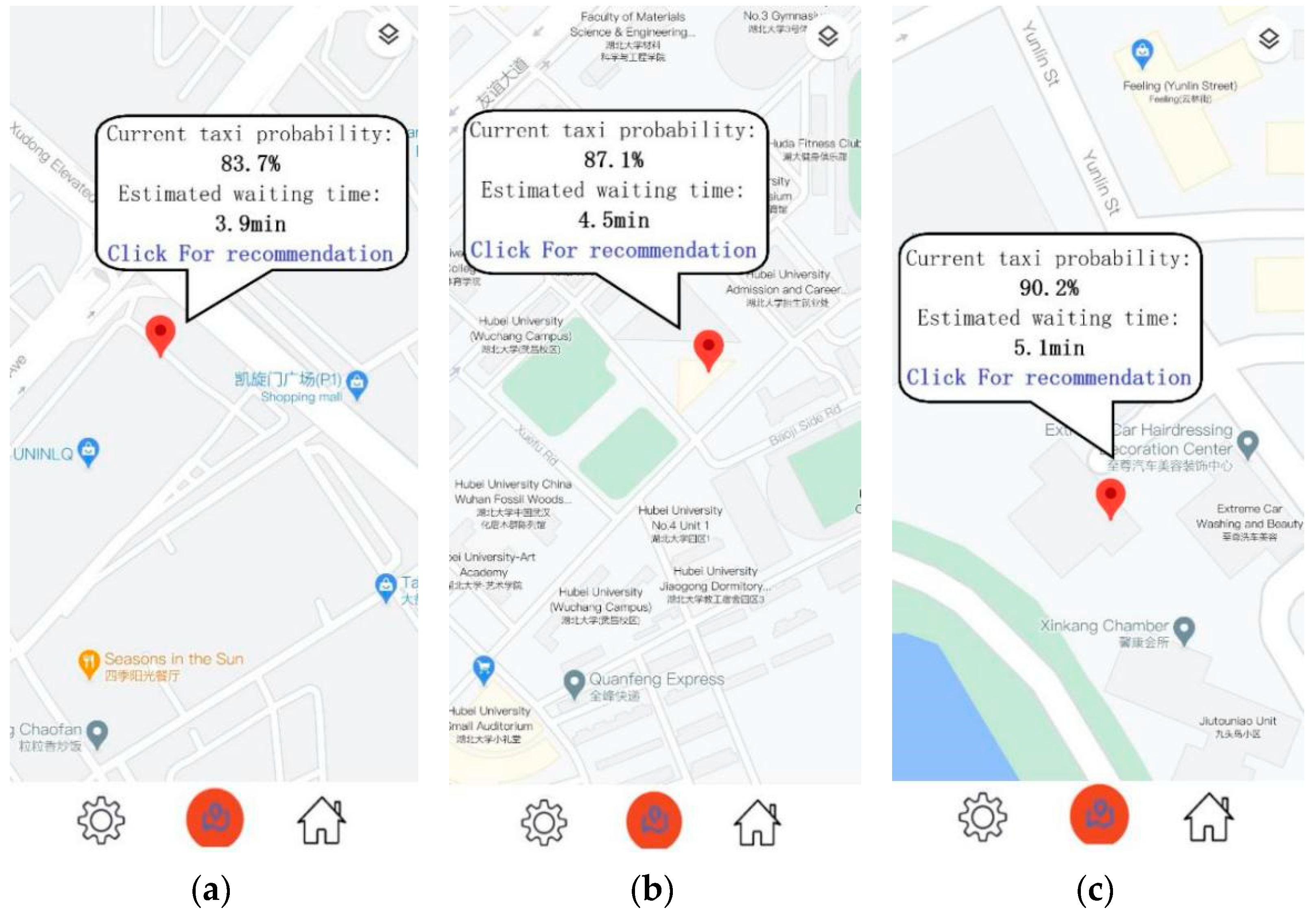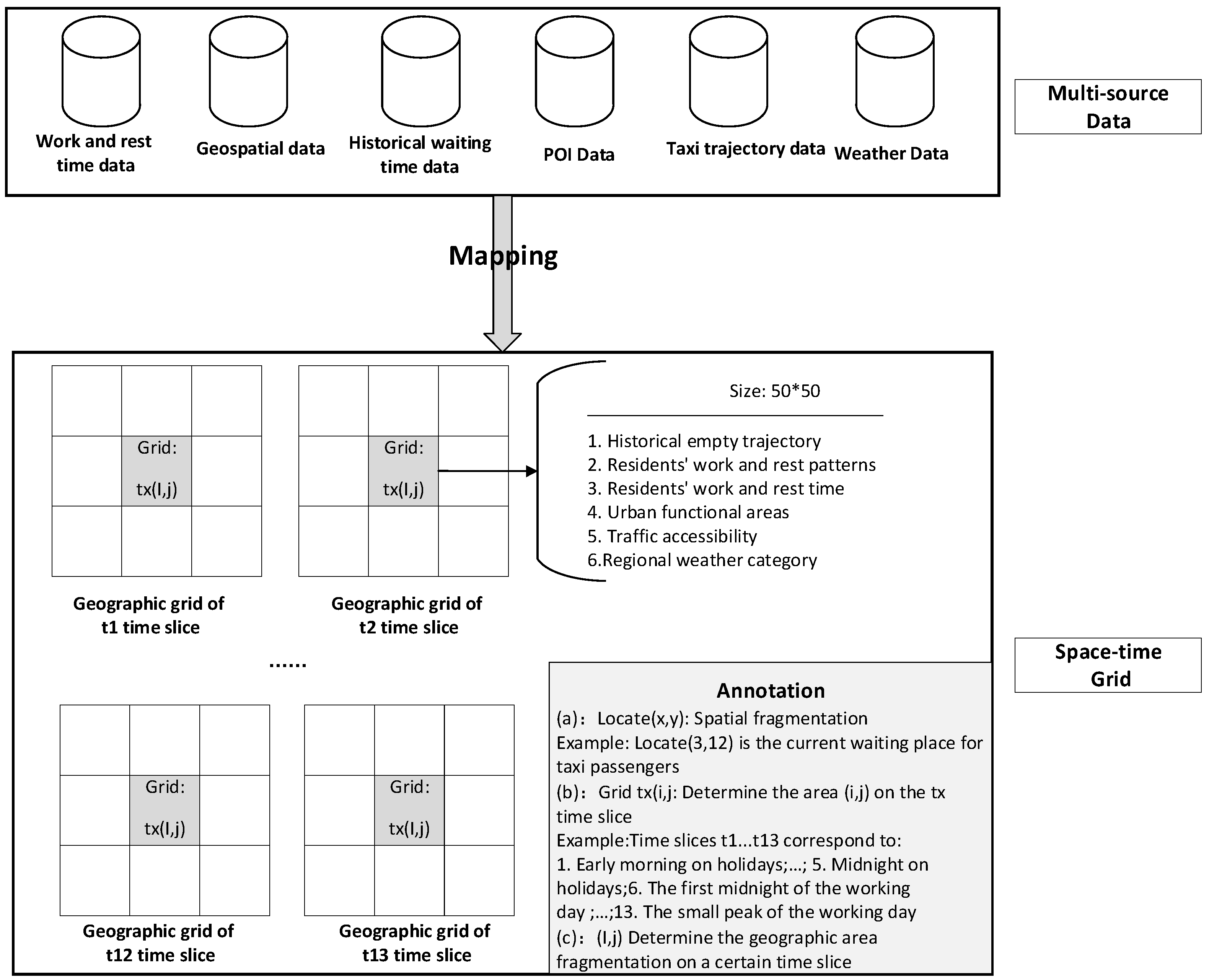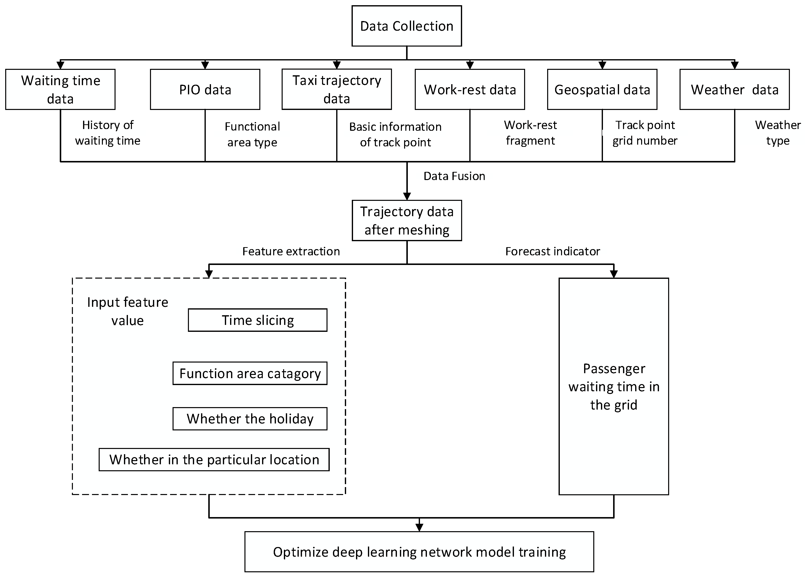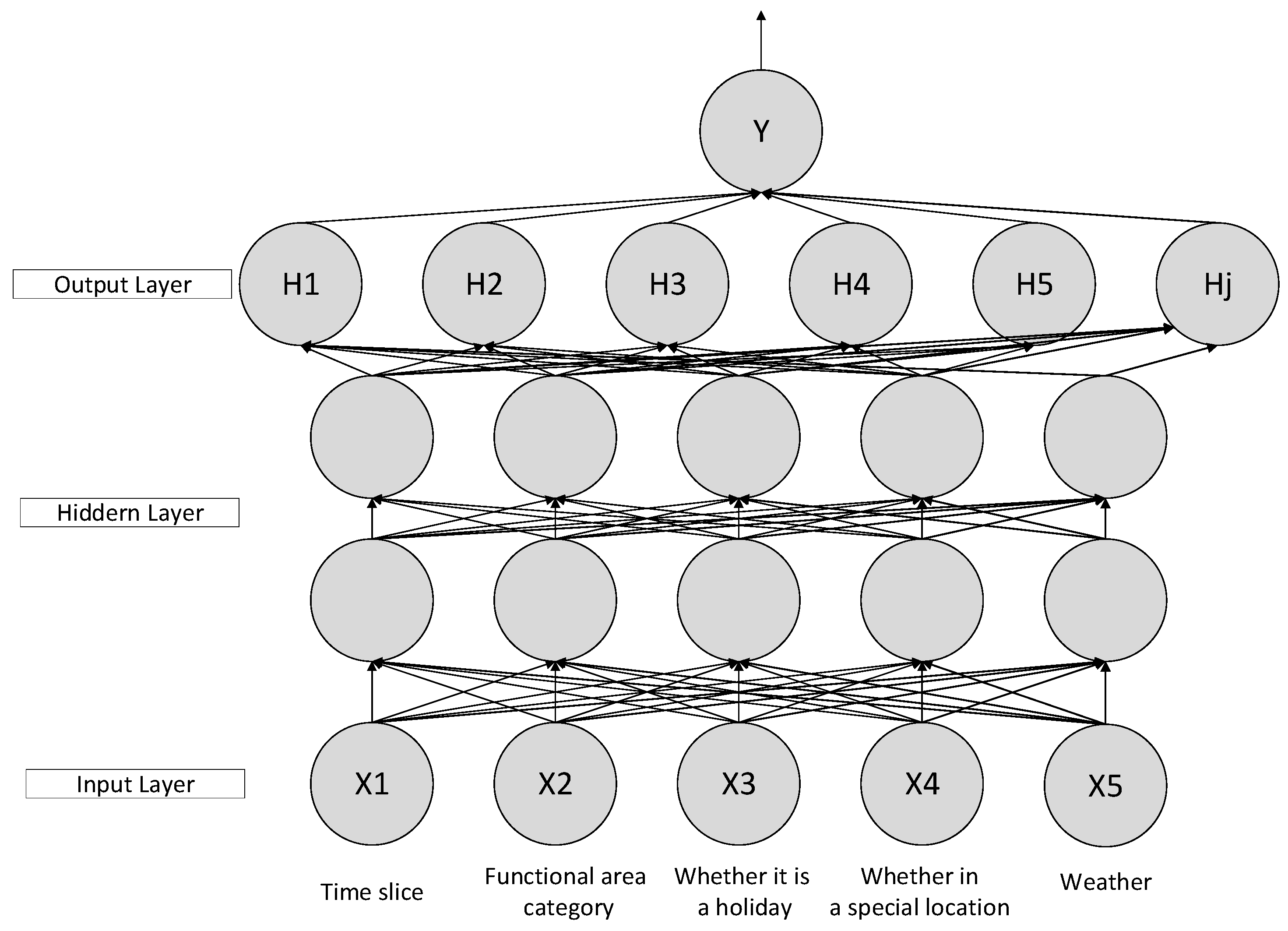However, there is often an imbalance between taxi supplies and demands, this leading in many cases to long waiting times and thus an urgent need for reasonable and effective automated solutions [3]. With the aim of bridging the gap between taxi demands and supplies with smart travels, this research introduces a neural network approach whose objective is to predict passengers’ taxi waiting times and provide passengers with optimized waiting places. Our approach is based on a combination of an optimized neural network, a grid-based spatio-temporal and functional structure of urban space and integration of multi-source data. Spatio-temporal and semantic data give the input of our modelling approach, from a selection of urban points of interest, historical taxi trajectory data including waiting times at specific locations and weather data. The whole approach is experimented in the Wuchang District of Wuhan in China using a set of real taxi trajectories recorded over a significant enough period of time and illustrated by a case study application that shows the interest of the whole modelling approach.

The rest of the paper is organized as follows. The next section provides a study of related work. Section 3 introduces the principles behind our behavioral model and develops the neural network modelling approach. Section 4 reports on the experimental results, while Section 5 draws the conclusions and suggests a few perspectives for further work.

2. Related Work

Nowadays, most urban taxis have GPS positioning systems make massive taxi trajectory data easily available. Massive taxi trajectory data contains valuable data on urban transportation patterns as well as driving behaviors, and then useful references for studying urban residents’ activities and giving a global picture of an urban transportation system. This led to the concept of “urban computing” that offers new computerized models of the city and further opportunities for mining and discovering urban trajectory patterns [4]. Indeed, before the emergence of smart cities, modelling and simulating urban taxi behaviors was, for instance, modelled using online algorithms and linear programming, taking into account taxi availabilities, pricing, number of passengers and waiting times [5]. Passenger flows between large urban areas were modelled using a demand–supply equilibrium of taxi services under competition and regulation and minimizing passenger waiting times [6].

With the development of IoT data, data-driven smart city computing has become an alternative promising resource for urban traffic flow analysis [7,8]. Incremental approaches based on historical taxi trajectory data can be applied to approximate both taxi demands and allocations to passengers [9]. Neural networks are also used to predict the demand for taxis to serve the drivers. In order to predict the demand of taxis to help drivers plan their routes, the CNN-BiLSTM attention neural network has been introduced to predict taxis demand [10]. Overall, it was shown that urban spatial-temporal flow prediction is of great importance to traffic management, land use, public safety, etc. Urban flows are affected by several complex and dynamic factors, such as patterns of human activities, weathers, events and holidays [11]. Modeling this type of data can be enhanced by deep learning approaches [12]. An attention-based convolutional recursive network was applied to predict taxi demands and correlate times and places [13].

Unlike demand forecasting, neural networks were hardly applied with multi-source data to forecast passengers’ waiting time. Nowadays, the most widely used method is to repair and analyze a taxi path based on GPS trajectory to predict taxi waiting times. For instance, a bus route map can be constructed and segmented, based on real-time bus GPS data to derive a path-based waiting time prediction [14]. A similar idea is used by applying three models to predict upstream bus routes separately to provide short-term forecasts for public transportation [15]. Large GPS trajectory data are empirically processed to derive taxi waiting time probabilities at some given locations and times [16]. Similarly, routing protocols and path-finding models are used as references for also deriving taxi waiting times at some given locations [17]. Elsewhere, the XGBoost algorithm is applied to predict static waiting times of taxis [18]. A crossroad network-based Markov decision process scheme is suggested to recommend taxi waiting place [19]. Recently, the importance of spatio-temporal features in traffic flow predictions is receiving more and more attention. The spatio-temporal features of the trajectory images are used in the prediction while the influence of space and weather are ignored [20]. GPS data is used to discover the impact of weather on human flow patterns [21]. The spatio-temporal semantics of the area are inferred to improve the accuracy [22]. Considering that a certain sequence may exist when people pass through the different geographic regions, time and space factors are utilized in learning the sequence rules of vehicles passing through different geographic functional regions [22].

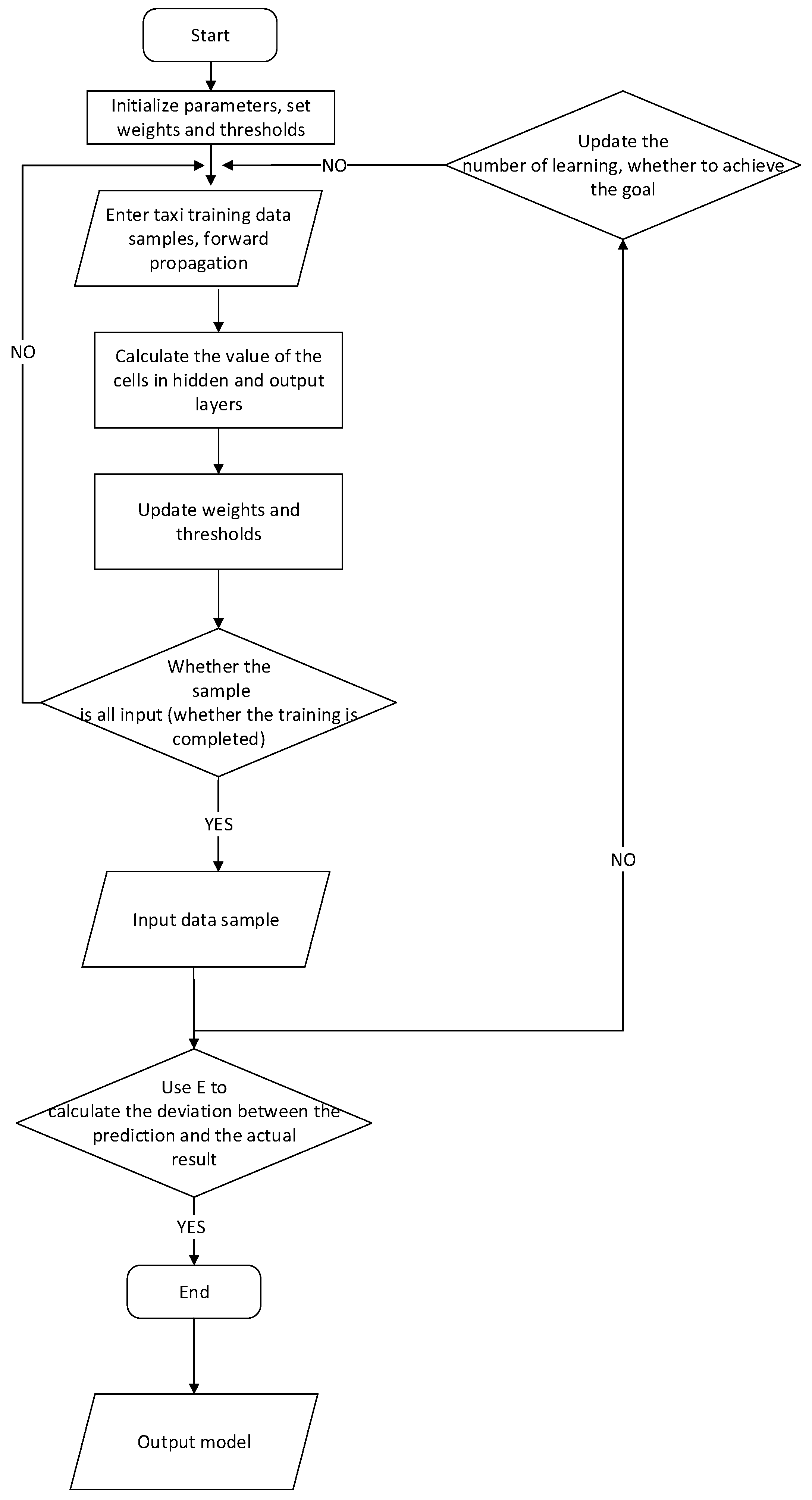
Overall, while there has been valuable progress in the way historical taxi trajectory data are combined with city traffic flow calculation, it appears that the accuracy of urban taxi waiting time prediction models still needs to be further improved. In particular, many factors are not taken into account, from taxi driving rules to passenger behavior in the city according to different timelines [23]. Furthermore, urban taxi drivers are rarely affected by dispatch centers, especially in China. In recent years, car-hailing apps appear as valuable solutions through which a passenger can directly order a taxi online. Taxi dispatching algorithm used in car-hailing apps have a great impact on the taxi running rules, which effectively reduced waiting times to a certain extent. The mode of demand–response (DR) taxi, such as Didi in China, UBER in the USA is able to show the waiting times for users, while this is the possible waiting time taken to drive from the location of the taxi whose driver is willing to go to the user’s place. The length of this waiting time in DR mode is decided by the distance between the responding taxi and user. Users always prefer to know the possible arrival time of the 1st empty taxi that is based on historic experiences. Learning taxi running rules from a large amount of historic taxi trajectory is a promising method for the waiting time prediction. This paper introduces a spatio-temporal schedule-based neural network model for urban taxi waiting time prediction. Based on the implicit influence of time, location, weather and urban residents’ daily schedules, the neural network was designed to learn taxi running rules for deriving the most accurate prediction of taxi waiting times.

3. Materials and Methods

3.1. Urban Residents’ Temporal Behavior

As previously mentioned, taxis play an important role in urban public transportation. Urban residents’ travel behaviors are directly associated with the taxis’ running laws in the city [24]. Such patterns generally reflect urban residents’ life, working habits, and studies among many activity categories. They are influenced by many factors that reflect human, urban, and socio-economical environments. Different human categories act in the city from state civil servants, business and administrative professionals, and students, retired people, and other professional categories [25,26]. Among many factors that impact taxi waiting times, residents’ working and leisure habits, and a distinction between different functional areas in the city constitute key factors. Moreover, the differences between working days, weekends and holidays are major criteria to consider [5,6]. All these parameters are considered by our neural network modelling framework, as well as functional and spatial differences in people’s behavior in the city. This leads us to setup different temporal interval divisions for holidays and working days to reflect differences in people’s behavior.

Without the loss of generality, we assume a temporal representation of residents’ behaviors in the city at the macro level as follows for either weekend or holidays:

• Between 05:00 to 08:59, in the early morning, most of the residents are resting at home while only a small number of them are active;
• From 09:00 to 13:59, when it comes to the morning to early afternoon rush, some of the residents are going out and performing some essential activities while others are staying at home;
• Between 14:00 and 17:59, it is afternoon peak, and residents generally have a need for some leisure activities such as shopping and dining;
• From 18:00 to 23:59, it is evening peak, including evening meals and travels back to home activities;
• From 24:00 to 04:59, people are generally sleeping at night peak.

Among many patterns that appear, students and working people generally have the relatively close distribution of activity patterns for a usual weekday [27]. During working days, and the night is divided into two parts, the first part is from 23:00 to 03:59, which means most of the residents are at their bedtime. The latter half of the night is from 04:00 to 06:59, called end of night. At the same time, some individual operators, such as breakfast shop operators, sanitation workers, and so on, have arrived at the time of business. Between 07:00 and 08:59, it is the first rush of urban residents’ daily travel, called the morning rush. In the meantime, both students and workers need to go to school and work. From 09:00 to 11:59, it is study time for students in school and office time for office workers in the company, and this time it is also working time for other occupations. Residents’ activities tend to be stable in that temporal period, which is the first flat peak period of urban residents’ daily work in a day. Then here comes the lunch break, which is from 12:00 to 14:29, people usually go for lunch or have a short time to go home. After that, between 14:30 and 17:30, it is afternoon time for school and work. Between 17:31 and 20:59, the second rush of the day is called the evening rush, the number of outdoor activities such as students leaving school, office workers returning home from work or shopping becomes larger. From 21:00 to 22:59, residents usually return home to rest after evening activities, ushering in the second small rush of the day, called late evening.

3.2. Urban Functional Distribution and Points of Interest in the City

An important assumption of our modelling approach to complement the temporal distribution of human activities developed in the previous section is to consider functional distribution and spatial structuration of the city layout. In order to do so, we consider the distribution of function points of interest in the city. Without the loss of generality, and to experiment our approach with real data, we integrate Gaode City POIs (points of interest) categorized into different activities, namely: shopping, education, commercial residences, scenery, catering, public facilities, transportation facilities, life, sports, medical treatment, government and accommodation. Based on this data, we further subdivided POIs into 19 kinds of categories: catering services, public facilities, shopping services, commercial housing and living services, sports leisure services, scenic spot, science and education, cultural services, private clinics and hospitals, accommodation services, government agencies and social organizations, companies, ATM and Banks, car parks, large commercial circle, large hospitals, large venues and bus stations. Since the activity rules of some large venues, such as stadiums, science and technology centers, children’s palaces, large business districts, scenic spots and general hospitals are highly dependent on holidays and working days, scenic spots, large venues, large business districts and general hospitals are classified as special functional areas. The resulting categories of POI are shown in

Table 1. Urban functional areas categories.

Functional Area Category	The Name of the Table	Whether Special Functional Area
Public utilities	poi_02_gonggongsheshi	No
Bus stations	poi_18_gongjiaozhan	No
Parking lots	poi_14_jiaotongsheshi	No
ATM and banks	poi_13_ATMyinhang	No
Government agencies and social groups	poi_11_zhengfujigou	No
Sports leisure services	poi_06_tiyuxiuxian	No
Life services	poi_05_shenghuofuwu	No
Food and beverage services	poi_01_canyin	No
Private clinics, specialist hospitals	poi_09_zhuangkeyiyuan	No
Companies	poi_12_gongsiqiye	No
Accommodation services	poi_10_zhusufuwu	No
Business residences	poi_04_shangwuzhuzhai	No
Science and education culture services	poi_08_kejiaowenhua	No
Shopping services	poi_03_gouwu	No
Scenic spots	poi_07_fengjing	Yes
Big business circles	poi_15_daxingshangquan	Yes
Large hospitals	poi_16_daxingyiyuan	Yes
Large venues	poi_17_daxingchangguan	Yes
No function area category identification	poi_19_null	No

below.

Since the same geographic grid location may have multiple functional area properties, the three dimensions of comprehensive economic gravity, traffic accessibility and financial connection network will determine the dominant weight of each type of functional area based on the premise of the interaction intensity of factors such as inter-city economic flow, people flow and logistics, and capital (financial) flow [28]. According to the weight of the dominant position in the unit grid, the functional area category of the grid is determined as its highest priority.

3.3. Analysis of Weather Affecting Taxi Passenger Behavior

Weather conditions are also important factors affecting the residents’ daily itineraries. People often choose whether to travel, the choice of means of travel and the arrangement of travel routes according to weather conditions [29]. Different weather will cause different fluctuations in the balance between the supply and demand of taxis and taxi passengers. Moreover, under the same weather, the behavior of passengers in different functional areas is likely to diverge. For example, residents in residential areas might less travel when it rains, thereby reducing the demand for taxis, while the demand for taxis in shopping service areas may surge.

Generally speaking, weather and temperature are important factors, for example, with sunny days, and residents have many choices of travel modes. People always choose to walk or share bicycles for short distances and choose urban rail transit or buses for longer distances. That is to say, the supply and demand relationship between taxis and passengers is in a relatively balanced situation on a sunny day. However, when the temperature reaches 35 °C or higher, residents are likely to reduce their trips and prefer taxis as convenient, flexible and not crowded. In rainy weather, residents’ travel time will increase, the willingness and frequency of travel will be weakened. At the same time, due to weather, the time and cost of the journey will also increase [30,31]. The amount of rainfall will also affect the behavior of taxi passengers. Light rain may promote the demand for taxis in large commercial districts, but heavy rain will have the opposite effect. In winter, it is difficult for road residents to travel in snowy cities, and the number of people who choose to travel by taxi will increase. Weather problems have aggravated road congestion and the situations in which vehicles are prone to slip and brake during driving, making it difficult for drivers to drive. Cloudy skies, fog, and hail can also affect the normal work of urban traffic, especially changing the daily demand for taxis by urban residents. When extreme weather occurs, urban traffic will fall into an abnormal state. For example, Wuhan experienced high temperatures, hail, and hurricanes on 11 August 2013, which negatively impacted citizens’ travel. In summary, this article divides the weather into ten categories: sunny, high temperature, overcast, light rain, moderate rain, heavy rain, snow, hail, fog, and extreme weather.

However, considering the relationship between weather and temperature, we only consider weather factors. On the one hand, weather suitable for travel is often accompanied by pleasant temperatures, and weather unsuitable for people to travel is often accompanied by severe temperatures. More importantly, the impact of weather on people’s travel is often greater. For example, even if the weather is pleasant, people are often reluctant to go out if it rains or is foggy. In summary, this model mainly uses weather factors to measure the impact of climate on people’s travel.

3.4. Multi-Source Data Fusion Based on a Spatio-Temporal Grid

3.4.1. Data Preprocessing

Evaluating the quality of incoming taxi trajectory data is a key issue to evaluate the accuracy and reliability of the developed model. Typical error data are as follows:

• Location error: GPS coordinate data are missing or gives an incoherent location;
• Speed error: a taxi speed exceeds a driving speed threshold;
• Data source error: data are not generated by a taxi GPS device;
• Status error: a taxi is in an ineffective state such as fortification and outage in taxi running.

The data preprocessing process first filters most common errors by observation and programming. After that, the application of Douglas–Peucker optimizes the trajectory point paths in order to resolve GPS drifts problems as suggested [32]. As illustrated in Figure 1, the track point P and the adjacent track points before and after it $P_p$,$P_n$ form a track triangle. The trajectory point P is projected onto the edge $P_n{P}_p$, and its projection length is H. If H is greater than the specified drift error, this point P is withdrawn. The drift error is set to the size of the map grid.

Then, the trajectory point P is projected onto the edge $P_n{P}_p$, and its projection length is H. If H is greater than the specified drift error, delete it. In this paper, the drift error is set to the size of the map grid.

3.4.2. Spatio-Temporal Grid Structuration

Considering the urban planning layout, geographical topography, resource allocation and other factors affecting the waiting time of taxi passengers, we choose to mesh the map into several grids of unit size [33,34]. Taking into account that, if the map grid is set too large, the actual meaning of the recommended waiting point will be lost. This is because, on the one hand, people are unwilling to move too far, and on the other hand, it takes too long to move to a better waiting point. Time is not necessarily the time difference between the two waiting points. When the map grid is set too small, the prediction may be inaccurate. This may be due to the small difference between the waiting time of the adjacent area or the unreachable location that is too close (if possible, in the house or the middle of the road, etc.). In view of the above considerations, this article sets the map grid size at 50 m × 50 m. The details of the map grid are shown in Figure 2 [35].

The minimum and maximum values of longitude and latitude in the grid are calculated based on the length and width of the grid and the longitude and latitude values of the center point of the grid, that is, the range of the grid. The form and meaning of grid information are shown in

Table 2. Map grid information data.

Field Name	Field Type	Description
fishnet_id	int (11)	Grid id number
POINT_X	double	Grid center point x-axis coordinate
POINT_Y	double	Grid center point y-axis coordinate/°
Longitude_min	decimal (10, 6)	The longitude of the grid/°
Longitude_max	decimal (10, 6)	The longitude of the grid/°
Latitude_min	decimal (10, 6)	The latitude of the grid/°
Latitude_max	decimal (10, 6)	The latitude of the grid/°

.

Table 3. Map grid information table data segment.

Fishnet_id	Longitude_min	Longitude_max	Latitude_min	Latitude_max
1	114.232525	114.234807	30.53251	30.534308
2	114.232974	114.235256	30.53251	30.534308
3	114.233424	114.235706	30.53251	30.534308
4	114.233873	114.236155	30.53251	30.534308
5	114.234322	114.236604	30.53251	30.534308

is a data fragment intercepted from the map grid information table read from the database.

The continuous trajectory of the taxi can be discretized by the grid operator of the administrative map. Match and compare the spatio-temporal data of waiting time data, POI data, taxi trajectory data, rest time data and geospatial data, so as to map the multi-source data to each grid respectively. The specific mapping method will be shown in Section 3.4.3.

3.4.3. Multi-Source Data Fusion

Taxi GPS data include taxi ID, recorded time, geographical location (longitude and latitude), driving speed, driving direction, passenger load and other information. A large number of taxi trajectory data with high accuracy, wide coverage and rich content have become an important data source for studying the travel rules of urban residents [16]. The common key taxi trajectory data structures are shown in

Table 4. Common taxi trajectory data table.

Field Name	Field Type	Description
T_TargetID	varchar (255)	Data id number
T_UTCT	decimal (15)	Timestamp(Unix)
T_Longitude	decimal (10, 6)	Longitude/°
T_Latitude	decimal (10, 6)	Latitude/°
T_Speed	decimal (10, 6)	Driving speed(km/h)
T_Heading	decimal (10, 6)	Driving direction/°
T_Status	decimal (10)	Driving status

.

Table 5. Common taxi trajectory data fragments.

T_TargetID	T_UTCT	T_Longitude	T_Latitude	T_Speed	T_Heading	T_Status
MMC8000GPSANDASYN051113-23416	1392235225	114.301990	30.606773	8.705277	28.17	262,144
MMC8000GPSANDASYN051113-24802	1392235226	114.285118	30.585786	8.391806	43.75	262,144
MMC8000GPANDASYN051113-22877	1392235226	114.279390	30.577443	0	0	0
MMC8000GPSANDASYN051113-22877	1392235225	114.279390	30.577443	0	0	262,144
MMC8000GPSANDASYN051113-22257	1392235225	114.345786	30.56768	10.719722	38.76	0
MMC8000GPSANDASYN051113-24534	1392235225	114.312878	30.540951	16.814444	13.71	262,144

shows some data fragments of common taxi trajectory data. Among them, T_Status means the taxi carrying passengers. As the value is 26,144, the taxi is carrying passengers, while the value is 0 means that the taxi is empty.

The continuous track of taxis is discretized by the grid operation of the administrative map. The waiting time data, POI data, taxi track data, work and rest time data and geospatial data are mapped to each grid according to the underlying spatio-temporal data, so that each grid unit contains the fused multi-source data. The details of the map are shown in Figure 3.

After cleaning and extracting historical waiting time data, POI data, taxi trajectory data, work and rest time data, and geospatial data, the entire map area is divided into a size of 50 m × 50 m, and each grid generates 13 grids. It is divided into time segments and includes five characteristic data: historical space trajectory, residents’ work and rest rules, residents’ work and rest time, urban functional areas, and traffic accessibility to form a multi-data space–time grid shown in Figure 4.

3.5. Spatio-Temporal Rules Neural Network Model

3.5.1. Neural Network Model Design

The waiting time of a taxi passenger can be approximated according to Equation (1).

$$t_{wait}=\frac{t-lo{c}_{first}-t_{current}}{num}*\sigma$$

(1)

In the equation, $t-lo{c}_{first}$ denotes the time for a passenger to encounter the first empty taxi at a given location $loc$. $t_{current}$ denotes the time point at which the current passenger is waiting for a taxi. $num$ denotes how many times an empty taxi appears at the current location and current time in historical taxi trail. σ is an empirical value, describing the relevance between $t-lo{c}_{first}$ and $t_{current}$. The value of σ ranges from 0 to 1. Without the loss of generality, σ is set to 1 based on practical experience.

In order to better adjust the number of hidden layers of the neural network, this study adjusted the settings for predicting positive examples. Normally, passengers can put up with the longest waiting time at about 2 min, and 30 s of waiting time enable passengers to have best experience. This paper assumes that if the difference between the predicted value and the actual value does not exceed 30 s, a positive example will be identified.

The neural network training model is optimized by the characteristics of waiting time, trajectory historical and POI data, behavioral and spatial data. The result will be taxi waiting times distributed along the grid spatial and temporal representation of the city. The time–space feature optimization neural network model is shown in Figure 5.

As demonstrated in related work, as long as there is a three-layer BP neural network with a hidden layer, any mapping function can be approximated [36]. We compare our neural network model results constrained by time and space features with up to four different hidden layers. It can be seen from

Table 6. Error table for different hidden layers.

Hidden Layer	1	2	3	4
Accuracy	92.5%	94.1%	93.3%	90%
Error	9.94 × 10−5	9.27 × 10−5	9.98 × 10−5	9.72 × 10−5

that the model with 2 hidden layers gave the highest accuracy.

Therefore, the model uses a BP neural network with a five-layer structure of fully connected, as shown in Figure 6 below.

The characteristic input values of the neural network model are represented by the main factors that influence the waiting time of taxi passengers in the grid as follows:

• X1 is the time slice corresponding to the urban residents’ daily schedule;
• X2 is based on POI data according to different urban functional area categories;
• X3 marks whether the day is a holiday;
• X4 determines whether the grid is in a particular location, such as a large business district, a large stadium and a general hospital.

The output layer is the output Y of the neuron, which reveals the time it takes for a passenger to wait at the grid for the first empty taxi. We use the ReLu function as the neural network activation function. Because of the linear characteristics of the ReLu function, the negative value of the function is 0, while the positive value does not change, i.e., one-sided suppression. The neurons in the neural network are also sparsely activated, making it easier to learn and optimize. For nonlinear functions, the ReLu function overcomes the vanishing gradient problem because the gradient of the non-negative interval is constant, so that the convergence speed of the model is maintained in a stable state. The ReLu function formula is shown in Equation (2).

$$\mathrm{ReLu}(x)=\max (0,x)$$

(2)

Adam is a first-order optimization algorithm for the iterative updating of neural network weights by training data. It occupies less memory during operation and has strong computing power, so it can replace traditional stochastic gradient descent and is suitable for solving large-scale data problems in the paper. The Adam algorithm is a random objective function-step optimization algorithm based on low-order adaptive moment estimation, and it is not easy to fall into the local optimum and has a fast update speed. Therefore, Adam uses the adaptive learning rate optimization algorithm to update the network parameters [37].

3.5.2. Model Prediction Process

The sections below introduce and analyze the characteristics of residents’ spatio-temporal behaviors according to the types of urban functional areas, and put forward the main factors affecting the taxi waiting times. A difference is made between working days or holidays, location and functional area types and POI where passengers are located and taken into account. These dynamic spatio-temporal environmental data directly affect the distribution of taxi carriage. The forecast flow chart for taxi passenger waiting times based on an optimized neural network is shown in Figure 7.

The forecasting process for the taxi passengers’ waiting times based on the spatio-temporal feature-optimized neural network model is as follows:

Step 1: First, initializes the network and normalize multivariate data.

Step 2: The neural network propagates forward to calculate the prediction of urban taxi waiting time.

Step 3: Use gradient drops to calculate the loss of each neuron.

Step 4: The neural network backpropagates the error information and updates the weights and biases of each neuron.

The Adam optimization algorithm was applied to update the network parameters.

4. Results and Discussion

4.1. Experimental Environment and Data Set

The hardware platform is an Intel (R) Core (TM), i7-8550U CPU s 1.80 HZ, windows 10, 8G memory. The experimental computing environment is Python 3.5, TensorFlow 1.7.0 and Keras framework.

Taxi trajectory data came from Wuchang District of Wuhan, Hubei Province, from 13 February 2014 to 19 February 2014, 6,705,086 taxi trajectory data were excluded in total by abnormal data cleaning, covering working days, holidays and special holidays (Valentine’s Day), which are typically representative and stable [38]. To reflect real-life situations better, we divided the test set and training set into two parts according to date. We divided the total 70-day trajectory data by date. The training set contains 60-day trajectory data, and the test set contains 10-day trajectory data.

Wuchang District’s geographical location is 114°14′ E–114°30′ E, 30°32′ N–30°37′ N, divided into 84,048 grids according to 50 m × 50 m units using ArcGIS10.3 [26]. There are 34,195 POI data in Wuchang. There are 6,705,086 trace data after the meshing of the permeation feature, of which 5,705,086 data are selected as training data, of which 1,000,000 data are used as test data. The test data is used as a sample data input for the trained BP neural network. The system is applied to different temporal periods and functional area taxi forecast, because the mean absolute error (MAE) intuitively reflects the deviation degree between the experimental prediction results and the actual value, so MAE evaluates the experiment results. The evaluation formula is as follows:

$$MAE=\frac{1}{N}{\displaystyle \sum _{i=1}^N\left|y_i-y_i^{\prime }\right|}$$

(3)

N represents the number of experimental results, $y_i$ indicates the actual time a given passenger waits for the first empty car, and $y_i^{\prime }$ indicates the prediction time for that passenger to wait until the first empty car.

4.2. Experiment Analysis and Discussion

4.2.1. Effect of Temporal Features on the Predictive Models

A total of 24 consecutive hours of the working day were divided into 8 time periods according to Section 3.1, and 24 consecutive hours during holidays that were divided into 5 time periods. The system predicts the waiting time for taxi passengers on weekdays and holidays. The MAE values are shown in

Table 7. MAE value of each time segment.

Time Lice	MAE (s)
work day: 4:00–6:59	71.32
work day: 7:00–8:59	56.78
work day: 9:00–11:59	24.12
work day: 12:00–14:29	21.5
work day: 14:30–17:29	30.96
work day: 17:30–20:59	33.85
work day: 21:00–22:59	19.67
work day: 23:00–3:59	34.63
holiday: 00:00–4:59	55.5
holiday: 5:00–8:59	37.49
holiday: 9:00–13:59	32.46
holiday: 14:00–17:59	34.33
holiday: 18:00–23:59	62.24

below, while the main patterns are illustrated in Figure 8.

It can be seen in Figure 8 that among the prediction effects of different time segments, the worst MAE value is 71.32 s, that is, passengers’ waiting time can be satisfactory predicted at any time segment. The average error of time prediction is always less than 1.5 min, and it can be considered that passengers can obtain reasonable predicted waiting time in different time periods.

Through the trend chart, one can find that whether it is a weekday or a holiday, the forecast error of the passenger waiting time during the day is relatively small. This may be caused by the relatively fixed behavior pattern of urban taxis during the day. Furthermore, the waiting time for taxis in the daytime itself may be less, so there will be no excessively large forecast deviations. In addition, in most time periods, the waiting time prediction error during holidays is higher than that of working days. The reason may be that different holidays have inconsistent influences on the behavior of taxis. For example, on National Day, a large number of foreigners will flood into the city, leading to a shortage of urban taxi supply. On the tomb-sweeping day, although residents travel more, there are fewer taxis as a way of travel, so the supply of taxis is excessive. Therefore, the further optimized model needs to analyze different holidays.

4.2.2. Effects of Spatial Dimension on the Predictive Models

The urban functional area is divided into 19 categories according as presented in Section 3.2. The model used in this paper predicts the waiting time of passengers according to different functional area categories, the MAE value of predicted passenger waiting times for different ribbon categories is shown in Figure 9 below.

As shown in Figure 8, the predicted MAE values of different functional areas are within a certain range, the highest MAE value is 73.28 s while the best one is only 17.68 s.

Among all the functional areas, locations close to taxi companies have the smallest error. This is because the mobility characteristics of taxis near companies are the most obvious whether on weekdays or holidays, so their taxi operation patterns are also the easiest to capture. As areas such as Government agencies and social groups, and bus stations are often located in remote locations with fewer taxis, the waiting time for taxis is thus longer and has strong randomness there. The prediction error is relatively big in such areas. Areas without function category identification are difficult to predict its taxi waiting time due to its fuzzy characteristics, so its prediction effect is worse than other areas.

To solve the relatively high prediction error of taxi duration near no function area category identification, the surrounding trajectory data can be used to model its urban functional attributes. Furthermore, trajectory data can fit such non-characteristic geographic areas by time periods to better simulate the real situation.

4.2.3. Effect of Weather Features on the Predictive Models

According to the provisions of Section 3.1, this paper divides the weather into 10 types. Under different weather conditions, the minimum MAE value of waiting time for taxi passengers predicted by this system is 24.05 and the maximum is 63.5. Moreover, the MAE value of predicted passenger waiting times for different weather is shown in Figure 10 below.

It appears that the more deeply the weather affects people’s lives, the greater the impact on the waiting time of taxis. There may be three reasons for this pattern. First of all, weather that causes less impact, such as sunny and cloudy days, will not bring major changes to the flow of taxis. Secondly, terrible weather is likely to increase taxi waiting times, so it is easier to predict with larger errors which cause the larger MAE value. In addition, extreme weather has less data, so its influence rules are difficult to learn by neural networks.

4.2.4. The Comparison of Prediction Results with Different Related Models

The algorithm model proposed in this paper is compared with the original unsolved three-layer BP neural network algorithm model mentioned in a related work widely applied [39], and to an algorithm based on empirical distribution prediction waiting time [16]. Hereafter, denoted as SF1, SF2 and SF3, respectively.

The SF3 algorithm predicts ride-hailing probability and waiting time based on the empirical distribution of historical data, and updates the model based on incremental learning. The initial estimate of the waiting time in a known time granularity unit is the mean value of the waiting time at the relevant time and place. For the new time granularity, the optimized waiting time prediction value is:

$$P_{i,j,d}^{new}=\frac{\rho \times {\widehat{P}}_{i,j,d}^{new}\times b+(1-\rho )\times P_{i,j,d}^{old}}{\rho \times b+(1-\rho )}$$

(4)

where ${\widehat{P}}_{i,j,d}^{new}$ is the initial estimated value of the waiting time in the new time granularity unit; $P_{i,j,d}^{old}$ is the optimized waiting time predicted value in the original data when no new data is added. b is the number of time granularities contained in the original data. The volatilization coefficient ρ is used to measure the importance of existing data and new data in the forecasting process.

In SF3, the feature point-location set and feature-time set are selected. The feature points are used to replace the adjacent data in GPS historical data (GPS historical data is transformed into a large number of feature point historical data). The waiting time of a feature space–time point is equal to the average of the data replaced by it in the original data. Therefore, the waiting time of each feature space–time point is calculated. A mapping model composed of the feature points and its waiting time is constructed. Then, the waiting time at a certain time and place can be predicted as the average of the waiting time of its adjacent characteristic time instants and space points. When the model needs to be updated due to new data, the waiting time of the feature–time–space points of the new data is calculated through the above process. Combining with t calculated from the old data. The new model is obtained according to the formula, where B is the number of feature points.

In order to enrich the feasibility of the experimental results, the experimental data is unified into 6,705,086 data with an accuracy rate added as one of the evaluation indicators.

$$acc=\frac{|w_t-w_p|}{w_t}\times 100\%$$

(5)

where $w_t$ represents the true value, $w_p$ denotes the model forecast value, and acc represents the accuracy of the model prediction results.

The MAE value and accuracy of the respective SF1, SF2 and SFF2 algorithm models are shown in Figure 11.

As shown in Figure 11, the experimental results exhibited by our optimized neural network SF1 give a MAE value of 58.7 and an accuracy rate of 92.4%. In contrast, the original unsolved three-layer BP neural network algorithm model, namely SF2, gives a MAE value of 112.3 and an accuracy of 58.3%, and finally, the model SF3 gives a MAE value of 76.6%, with an accuracy rate of 68.6%. Compared to the basic BP network, the approach developed in this paper considers additional time and space constraints, thus explicitly modeling taxi waiting time patterns, so the final accuracy rate is higher. As for SF3, although the trajectory of urban taxis reflects a certain trend, its randomness is still very large for some locations. The neural network that integrates multi-source data and is constrained by temporal and spatial rules and then can better model taxi waiting rules in every corner of the city. In summary, the very probable reason for this output lies in the full integration of the behavioral and spatio-temporal characteristics of the city layout and the computational efficiency of the neural network model.

4.3. Prototype Application

In order to illustrate and visualize the potential of our model, a prototype application for taxi supply demand has been developed in the city of Wuhan. The objective of the application is to integrate some user’s spatio-temporal data to provide the application with waiting time predictions for some given user and taxi locations. The software architecture diagram is shown in Figure 12 below.

Overall, one might note as far as the neural network is appropriately trained, computational times are relatively efficient as demonstrated by the application experiments developed so far. As shown in Figure 13, passengers who take a taxi in front of the university at noon are expected to wait 4.5 min before the first empty taxi can pass, with an accuracy rate of 87.1%; passengers who take a taxi in front of the community at midnight are expected Wait 5.1 min for the first empty taxi to pass, with an accuracy rate of 83.7%; passengers who take a taxi before the mall at 3 pm are expected to wait 3.9 min for the first empty taxi to pass, with an accuracy rate of 91.3%. Based on the waiting time prediction and sorting time, the prototype application further suggests the ride point with the highest success rate.

5. Conclusions and Future Work

Over the past few years, the emergence of many sensor-based applications in urban environments progressively favors the emergence of the concept of smart cities. Among a wide range of novel services offered to urban residents and decision-makers, transportation on demand has radically changed the way operations are distributed amongst potential passengers and delivery companies. When considering and modelling taxi demand and supplies, many factors impact the waiting times of taxi passengers, from the efficiency of the urban network infrastructure to the functional organization of the city, to the optimization of taxi resources and passenger pickup locations, to traffic flows to mention a few examples [40].

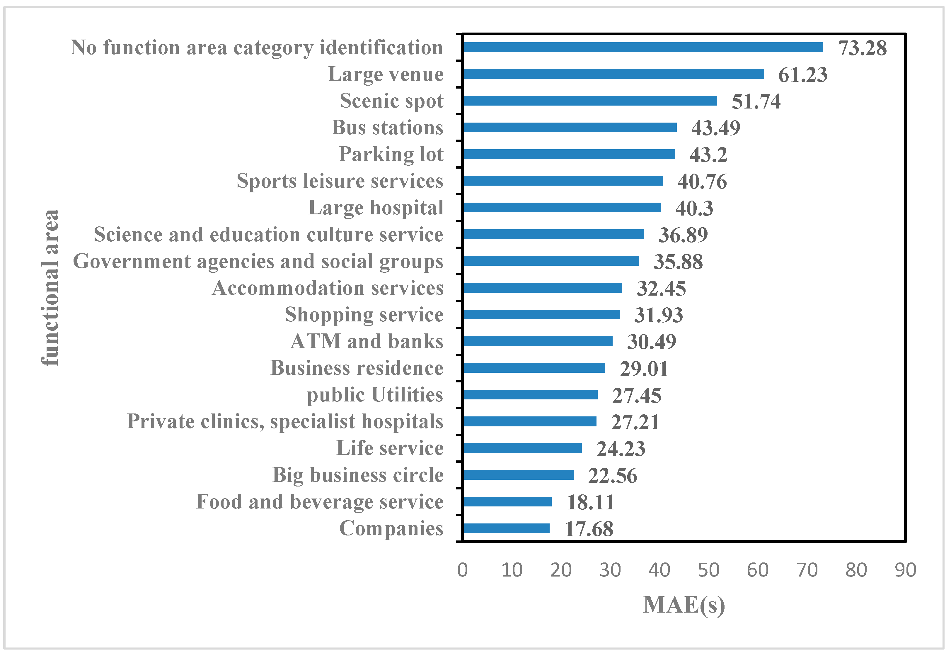
The research developed in this paper introduced an experimental neural network model whose objective is to predict and optimize taxi allocation times to passenger demands in an urban environment. The approach is based on a close integration of multi-dimensional data, from historical taxi trajectories, to a spatio-temporal distribution of human behaviors in the city according to different functional, temporal constraints and weathers. The applicability, accuracy and effectiveness of the proposed model are primarily compared with actual historical taxi trajectory data and a spatio-temporal behavioral model of urban residents. Lastly, the whole neural network approach is compared to a few alternative modelling approaches. We conducted experiments with 70 days of taxi trajectory data in Wuhan. The experimental results show that under the weather at any time and place, the MAE value of the prediction result of this model is less than 73.27, and the RSME value is less than 7.33. The results also show that our modelling approach performs relatively well in terms of accuracy and efficiency.

The advantage of this modelling approach is twofold: it can help taxi drivers to reduce the no-load rate while reducing waste of energy resources, and it can improve the balance between the supply and demand of taxis and passengers to some extent this being a key issue in taxi demand allocation tasks [40]. For passengers, predicting the waiting time in advance can also improve the success rate of taking a taxi and help passengers arrange their journey appropriately.

Although the research has made some preliminary progress, additional issues need to be further developed. Subsequent work will continue around the following three points: first by further optimizing the time–space modeling, such as different holidays and area without function category identification. Secondly, based on predicted taxi waiting times, the optimization of allocation pickup points might be still explored with further algorithmic approaches. Third, the generalization performance will be in consideration.

References

1. Tang, T.; Liu, R.; Choudhury, C. Incorporating weather conditions and travel history in estimating the alighting bus stops from smart card data. Sustain. Cities Soc. 2020, 53, 101927. [Google Scholar] [CrossRef]
2. Shi, J.; Mao, J.; Jin, C. Travel time prediction for urban road based on spatial-temporal dependency. J. Syst. Simul. 2017, 29, 2309. [Google Scholar]
3. Wang, Y.; Shan, X.; Meng, Y. Inter-regional accessibility evaluation model of urban based on taxi GPS big data. Comput. Sci. E 2019, 46, 278–284. [Google Scholar]
4. Zheng, Y. Overview of urban computing. Geomat. Inf. Sci. Wuhan Univ. 2015, 40, 1–13. [Google Scholar]
5. Deng, C.; Ong, H.; Ang, B.; Goh, T.N. A Modelling study of a taxi service operation. Int. J. Oper. Prod. Man. 1992, 12, 65–78. [Google Scholar] [CrossRef]
6. Yang, H.; Wong, S.; Wong, K.I. Demand-supply equilibrium of taxi services in a network under competition and regulation. Transport. Res. B Meth. 2002, 36, 799–819. [Google Scholar] [CrossRef]
7. Alam, F.; Mehmood, R.; Katib, I.; Albogami, N.N.; Albeshri, A. Data Fusion and IoT for Smart Ubiquitous Environments: A Survey. IEEE Access 2017, 5, 9533–9554. [Google Scholar] [CrossRef]
8. Haydari, A.; Yilmaz, Y. Deep Reinforcement Learning for Intelligent Transportation Systems: A Survey. arXiv 2020, arXiv:2005.00935. [Google Scholar]
9. Luis, M.; Joao, G.; Michel, F.; João, M.; Luis, D. On predicting the taxi-passenger demand: A real-time approach. Encontro. Port. Inteligência Artif. 2013, 54–65. [Google Scholar]
10. Veres, M.; Moussa, M. Deep Learning for Intelligent Transportation Systems: A Survey of Emerging Trends. IEEE Trans. Intell. Transp. Syst. 2019, 21, 3152–3168. [Google Scholar] [CrossRef]
11. Guo, X. Prediction of Taxi Demand Based on CNN-BiLSTM-Attention Neural Network. Int. Conf. Neural Inf. Process. 2020, 12534, 331–342. [Google Scholar]
12. Xie, P.; Li, T.; Liu, J.; Du, S.; Yang, X.; Zhang, J. Urban flows prediction from spatial-temporal data using machine learning: A survey. arXiv 2019, arXiv:1908.10218. [Google Scholar]
13. Liu, T.; Wu, W.; Zhu, Y.; Tong, W. Predicting taxi demands via an attention-based convolutional recurrent neural network. Knowl. Based Syst. 2020, 206, 106294. [Google Scholar] [CrossRef]
14. Ma, J.; Chan, J.; Ristanoski, G.; Rajasegarar, S.; Leckie, C. Bus travel time prediction with real-time traffic information. Transp. Res. Part C Emerg. Technol. 2019, 105, 536–549. [Google Scholar] [CrossRef]
15. Petersen, N.C.; Rodrigues, F.; Pereira, F.C. Multi-output Deep Learning for Bus Arrival Time Predictions. Transp. Res. Procedia 2019, 41, 138–145. [Google Scholar] [CrossRef]
16. Wang, Z.Y.; Li, T.R.; Cheng, R.; Wang, Y.; Yi, X.W. Prediction of probability of hitting vacant taxi and waiting time based on empirical distribution. Comput. Eng. Appl. 2015, 51, 254–259. [Google Scholar]
17. Zhu, D. Research on routing protocol and route-decision model of vehicular ad-hoc Networks. Harbin Inst. Technol. 2014, 1, 11–13. [Google Scholar]
18. Kankanamge, K.D.; Witharanage, Y.R.; Withanage, C.S.; Hansini, M.; Lakmal, D.; Thayasivam, U. Taxi Trip Travel Time Prediction with Isolated XGBoost Regression. In Proceedings of the 2019 Moratuwa Engineering Research Conference (MERCon), Moratuwa, Sri Lanka, 3–5 July 2019. [Google Scholar]
19. Rong, H.; Zhang, X.; Li, Z.; Ai, Z. Waiting or Moving? A Crossroad Network-Based Markov Decision Process Approach to Catch Vacant Taxis. IEEE Access 2020, 8, 10528–10542. [Google Scholar] [CrossRef]
20. Sun, S.; Wu, H.; Xiang, L. City-Wide Traffic Flow Forecasting Using a Deep Convolutional Neural Network. Sensors 2020, 20, 421. [Google Scholar] [CrossRef] [PubMed] [Green Version]
21. Nawaz, A.; Zhiqiu, H.; Senzhang, W.; Hussain, Y.; Khan, I.; Khan, Z. Convolutional LSTM based transportation mode learning from raw GPS trajectories. IET Intell. Transp. Syst. 2020, 14, 570–577. [Google Scholar] [CrossRef]
22. Kuang, L.; Hua, C.; Wu, J.; Yin, Y.; Gao, H. Traffic Volume Prediction Based on Multi-Sources GPS Trajectory Data by Temporal Convolutional Network. Mob. Netw. Appl. 2020, 25, 1405–1417. [Google Scholar] [CrossRef]
23. Lam, H.; Diaz-Aviles, E.; Pascale, A.; Gkoufas, Y.; Chen, B. (Blue) Taxi destination and trip time prediction from partial trajectories. In Proceedings of the International Conference on ECML PKDD Discovery Challenge, Porto, Portugal, 7–11 September 2015. [Google Scholar]
24. Ma, X.; Yu, H.; Wang, Y.; Wang, Y. Large-scale transportation network congestion evolution prediction using deep learning theory. PLoS ONE 2015, 10, e0119044. [Google Scholar] [CrossRef] [PubMed]
25. Han, B.; Wang, Z.; Jin, B. An anomaly detection algorithm for taxi based on trajectory data mining and online real-time monitoring. J. USTC 2016, 46, 247–252. [Google Scholar]
26. Fu, X.; Sun, M.; Sun, H. Taxi commute recognition and temporal-spatial characteristics analysis based on GPS data. China J. Highw. Transp. 2017, 30, 134–143. [Google Scholar]
27. Qi, H.X.; Chen, L.Z. Study of temporal and spatial characteristics of students’ behavior in Hangzhou Xiasha higher education eastern park. Geogr. Res.-Aust. 2010, 7, 1281–1290. [Google Scholar]
28. Lee, J. Analysis on the waiting time of empty taxis for the taxi telematics system. In Proceedings of the 3rd International Conference on Convergence and Hybrid Information Technology, Busan, Korea, 11–13 November 2008; Volume 1, pp. 66–69. [Google Scholar]
29. Kang, C.; Liu, X.; Xinyue, X.U.; Qin, K. Impact of Weather Condition on Intra-Urban Travel Behavior: Evidence from Taxi Trajectory Data. J. Geo-Inf. Sci. 2019, 21, 118–127. [Google Scholar]
30. Hranac, R.; Sterzin, E.; Krechmer, D.; Rakha, H.; Farzaneh, M. Empirical Studies on Traffic Flow in Inclement Weather. Floods 2006, 385, 1–107. [Google Scholar]
31. Gong, D.P.; Song, G.H.; Li, M.; Gao, Y.; Yu, L. Impact of Rainfalls on Travel Speed on Urban Roads. J. Transp. Syst. Eng. Inf. Technol. 2015, 15, 218–225. [Google Scholar]
32. Douglas, D.H.; Peucker, T.K. Algorithms for the reduction of the number of points required to represent a digitized line or itscaricature. Can. J. Cardiol. 1973, 10, 112–122. [Google Scholar]
33. Qi, G.D.; Pan, G.; Li, S.J.; Wu, Z.; Zhang, D.; Sun, L.; Yang, L. How long a passenger waits for a vacant taxi-large-scale taxi trace mining for smart cities. In Proceedings of the IEEE International Conference on Green Computing & Communications, Beijing, China, 20–23 August 2013. [Google Scholar]
34. Qi, G.D.; Li, S.J.; Pan, Y.; Pan, G. Human-Machine Environment (HHME 2012) PCC. In Proceedings of the 8th Harmony Conference on Harmony, Guangzhou, China, 29–31 May 2012. [Google Scholar]
35. Sun, R. Real-Time Prediction of Hot Spots Based on Trajectory and POl Data; Jilin University: Jilin, China, 2017. [Google Scholar]
36. Ji, F. Neural Computing Intelligence Foundation; Southwest Jiaotong University Press: Chengdu, China, 2000. [Google Scholar]
37. Kingma, D.P.; Ba, J. Adam: A method for stochastic optimization. arXiv 2014, arXiv:1412.6980. [Google Scholar]
38. Kang, Y.H.; Wang, Y.Y.; Xia, Z.J.; Chi, J.; Jiao, L.M.; Wei, Z.W. Identification and classification of Wuhan Urban Districts based on POI. J. Geomat. 2018, 43, 81–85. [Google Scholar]
39. Jindal, I.; Qin, T.; Chen, X.W.; Nokleby, M.; Ye, J.P. A unified neural network approach for estimating travel time and distance for a taxi trip. arXiv 2017, arXiv:1710.04350. [Google Scholar]
40. Mao, Y.C.; Chen, Y. Uncertain vehicle intersection trajectory prediction. Comput. Sci. 2018, 45, 235–240. [Google Scholar]
Figure 1. Track triangle for checking the drift track points.
Ijgi 10 00703 g001
Figure 2. Mapping grid structure.
Ijgi 10 00703 g002
Figure 3. Multi-source data fusion.
Ijgi 10 00703 g003
Figure 4. Multi-source data fusion method.
Ijgi 10 00703 g004
Figure 5. Time–space feature optimization neural network model principles.
Ijgi 10 00703 g005
Figure 6. Topological structure of the neural network.
Ijgi 10 00703 g006
Figure 7. Spatio-temporal feature optimization neural network flow.
Ijgi 10 00703 g007
Figure 8. Prediction effect of different time segments.
Ijgi 10 00703 g008
Figure 9. Prediction effect of different functional areas.
Ijgi 10 00703 g009
Figure 10. Prediction effect of different weather features.
Ijgi 10 00703 g010
Figure 11. Experimental result graphs of different algorithm models.
Ijgi 10 00703 g011
Figure 12. Software architecture diagram.
Ijgi 10 00703 g012
Figure 13. (a) Application used in front of the university at 12 noon; (b) application used in front of the community at 12 midnight; (c) application used before the mall at 3 pm.
Ijgi 10 00703 g013