Regression and Evaluation on a Forward Interpolated Version of the Great Circle Arcs–Based Distortion Metric of Map Projections

Abstract

We studied the numerical approximation problem of distortion in map projections. Most widely used differential methods calculate area distortion and maximum angular distortion using partial derivatives of forward equations of map projections. However, in certain map projections, partial derivatives are difficult to calculate because of the complicated forms of forward equations, e.g., equations with iterations, integrations, or multi-way branches. As an alternative, the spherical great circle arcs–based metric employs the inverse equations of map projections to transform sample points from the projection plane to the spherical surface, and then calculates a differential-independent distortion metric for the map projections. We introduce a novel forward interpolated version of the previous spherical great circle arcs–based metric, solely dependent on the forward equations of map projections. In our proposed numerical solution, a rational function–based regression is also devised and applied to our metric to obtain an approximate metric of angular distortion. The statistical and graphical results indicate that the errors of the proposed metric are fairly low, and a good numerical estimation with high correlation to the differential-based metric can be achieved.

1. Introduction

A geographic map is a planar symbolic depiction describing natural or social features and characteristics on Earth or other planets [1]. In the process of map making, map projections [2,3,4,5] are fundamental because they represent an accurate transformation between three-dimensional and planar coordinates.

Over the last two thousand years, several map projections have been proposed. Map construction methods involve geometry projections, mathematical constructions [6,7,8,9], transformation and combinations [10,11,12,13,14,15], and approximation and optimization [16,17,18,19]. Modern computer software and libraries are also available for cartography and coordinate transformations, e.g., NASA’s G.Projector and Open Source Geospatial Foundation’s PROJ library [20,21].

As spheres and ellipsoids are not developable surfaces, distortions in map projections are inevitable [22,23]. The measurement and analyses of distortions [24,25] for different types of map projections are critical and still a challenging task for the design [16], categorization, evaluation, comparison, selection [26,27], and optimization [19] of map projections.

Nicolas Tissot devised a visual indicator (i.e., Tissot’s indicatrix or Tissot’s ellipse) to represent linear, angular, and areal distortion in map projections [28,29]. Many authors derived different computational formulae of Tissot’s original theory [28] in the numerical details [24,30]. Among the different forms of equations, area distortion and maximum angular distortion are calculated by the partial derivatives of forward equations (see p. 24 in [2]), and they are used as the reference of our metric.

The singular value decomposition (SVD)-based method [30] employs an algebraic approach. The SVD-based method can alternatively be used to calculate the same results as the maximal and minimal linear scales at a given point. There are also several metrics proposed based on partial derivatives. For example, the large-scale distortions of flexion and skewness are defined as Goldberg–Gott indicatrices [31,32].

Further, there are some global distortion metrics for an overall comparison of map projections [24,25]; e.g., Airy–Kavrayskiy metric [25] and differential-derived Capek Q [33].

However, above the Airy–Kavrayskiy metric, Goldberg-Gott indicatrices, Capek Q, and the SVD-based methods are all dependent on partial derivatives of forward or inverse equations of map projections.

Partial derivatives of forward equations are not always yielded in convenient ways. For example, Mollweide, Boggs Eumorphic, Eckert IV, Nell, and Putniṇš $P_2$ projections do not have the closed-form of forward equations, and they require iterative computations [2,34], such as Newton–Raphson iterations. In addition, certain projections may be interrupted (e.g., Hierarchical Equal Area isoLatitude Pixelisation, or HEALPix [35,36], interrupted Goode homolosine [22,23,37] and icosahedral Snyder equal area [38] projections), derivative discontinuous (e.g., uninterrupted Goode homolosine [14] and Robinson [39] projections), have singularity points (Mercator and Peirce Quincuncial [40] projections), or may have an elliptic integral (Adams World in a Square I and II and Peirce Quincuncial [40] projections) in forward equations. Another complicated example is the Chamberlin trimetric projection [41], which has multiple loops and several if–else branches in forward equations in the implementation of PROJ library. The above projections and similar cases indicate that calculating partial derivatives, as well as the differential metric and its derivatives, for map projections is not always an easy task.

In addition to map projections defined using mathematical formulae, tessellation using direct spherical subdivision (DSS) produces discrete global grids [42,43]. DSS methods are recursive subdivisions; hence, there is no explicit form of transformations between the geographic coordinate system and grid coordinate system. Consequently, the differential methods and its derivatives are not applicable to DSS-based grids [44].

The averaged ratio metric between complementary profiles [44] is based on spherical small circle arcs (SCA). SCA-based metrics and their derived spherical great circle arc (GCA)-based indicators [45] are all differentially independent. These methods sample points on the projection plane and transform sample points from the projection plane to the sphere to calculate SCA- or GCA-based metrics. The primary benefit of SCA- or GCA-based metrics includes independence from differential-based calculation. However, one shortcoming is their dependency on inverse equations of map projections. Nonetheless, certain map projections do not have explicit forms of inverse equations, such as Apian Globular I, Bacon Globular, Ortelius oval, Denoyer semi-elliptical, Ginsburg VIII, Laskowski, and Larrivée projections. Implicit forms of inverse equations for these map projections are also difficult to derive. This is a restriction of SCA- or GCA-based metrics when evaluating map projections without explicit or implicit forms of inverse equations.

In this paper, we extend the inverse equation-dependent GCA-based metric [45] to a forward interpolated form that is solely dependent on the forward equations of map projections. The proposed metric is abbreviated as forward GCA (FWD–GCA) for conciseness. The FWD–GCA approach samples points on the sphere, and transforms these sampled points to a projection plane. Then, the vector interpolation is applied to the sample points on the sphere to obtain a new set of sample points to create the new projected points on the projection plane that satisfies the orthogonal conditions of the GCA-based metric.

Regression between the FWD–GCA metric and differential-based maximum angular distortion was also studied. For achieving a high precision of regression, rational functions with degree one were employed, and the relationship among regression coefficients was studied and determined.

The FWD–GCA metric is derived and implemented for the unit sphere in this paper. Under the assumption of the spherical Earth, one known shortcoming of the FWD–GCA metric is that it is currently unsuitable for ellipsoidal map projections.

The remainder of this paper is organized as follows. Relevant studies related to differential methods and GCA-based metrics are outlined in Section 2. The FWD–GCA metric, and the process of calculation and interpolation are introduced in Section 3. Regressions by employing linear and rational functions are established and presented in Section 4. The experiments and validation are shown in Section 5. In Section 6, selected map projections are evaluated and compared. Finally, Section 7 discusses the results and concludes this paper.

2. Related Work

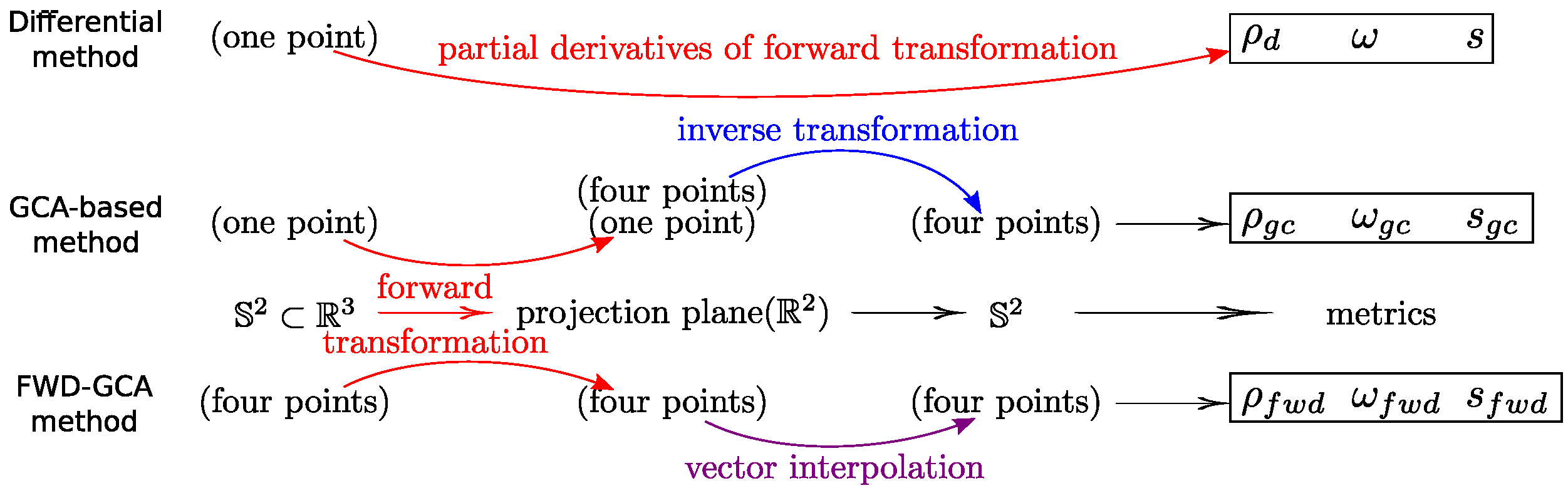
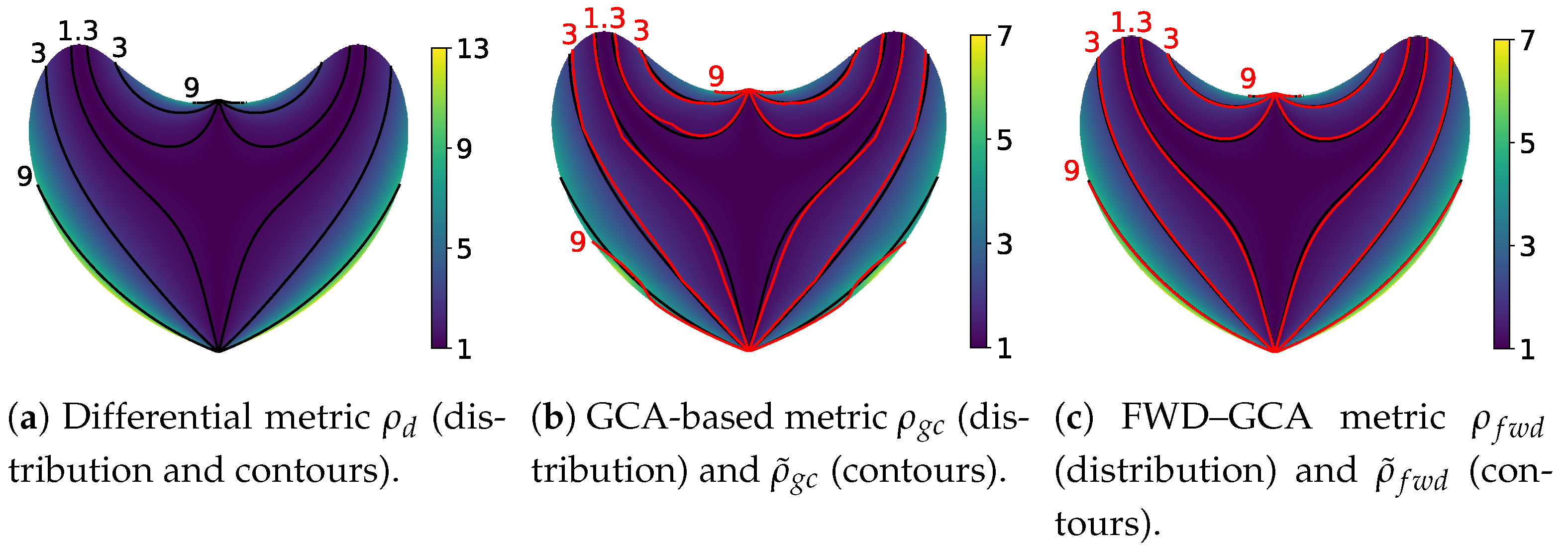
2.1. Differential Metric

Given partially differentiated forward equations $x(\phi ,\lambda )$ and $y(\phi ,\lambda )$ of a map projection, where $\phi$ and $\lambda$ represent the latitude and longitude, respectively, and x and y represent the projected coordinates, the differential metric (see p. 24 in [2]) calculates the maximum angular distortion $\omega$ (see Equation (6)) and area distortion s (see Equation (9)) for the projections on the sphere. Metric $\omega$ represents the greatest deviation from the correct angle in Tissot’s indicatrix. The implementation of the differential metric in Julia is provided in Codes S1 (for map projections with the explicit form of forward equations) and S2 (for map projections with the implicit form of forward equations) in supplementary materials. For the simplicity of presentation, the formulae for the differential metric (see Equations (1)–(9)), GCA-based metric (see Section 2.2), and FWD–GCA metric (see Section 3) are defined on a unit sphere ${\mathbb{S}}^2$ centered at origin O.

$$h=\sqrt{{\left(\frac{\partial x}{\partial \phi }\right)}^2+{\left(\frac{\partial y}{\partial \phi }\right)}^2},$$

(1)

$$k=\frac{1}{cos\phi }\sqrt{{\left(\frac{\partial x}{\partial \lambda }\right)}^2+{\left(\frac{\partial y}{\partial \lambda }\right)}^2},$$

(2)

$$sin{\theta }^{\prime }=\frac{1}{hkcos\phi }\left(\frac{\partial y}{\partial \phi }\frac{\partial x}{\partial \lambda }-\frac{\partial x}{\partial \phi }\frac{\partial y}{\partial \lambda }\right),$$

(3)

$$a^{\prime }=\sqrt{h^2+k^2+2hksin{\theta }^{\prime }},$$

(4)

$$b^{\prime }=\sqrt{h^2+k^2-2hksin{\theta }^{\prime }},$$

(5)

$$\omega =2arcsin\left(\frac{b^{\prime }}{a^{\prime }}\right),$$

(6)

$$a=\frac{a^{\prime }+b^{\prime }}{2},$$

(7)

$$b=\frac{a^{\prime }-b^{\prime }}{2}.$$

(8)

$$s=ab=hksin{\theta }^{\prime },$$

(9)

where h and k represent scale factors along the meridian and the parallel, respectively; a and b represent the maximum and minimum linear scale factors, respectively; $\omega$ denotes the maximum angular distortion; and s represents the areal scale factor [2,25,32].

The maximum angular distortion $\omega$ and area distortion s are used as reference metrics (see Section 4 and Section 5) for evaluating the GCA-based and FWD–GCA metrics in this paper.

Using differential-based metrics is straightforward for map projection with explicit forward equation (see Code S1). However, the Newton–Raphson iteration is needed for map projections with implicit forward equations (see Code S2); the derivation of partial derivatives is also required (see Appendix A).

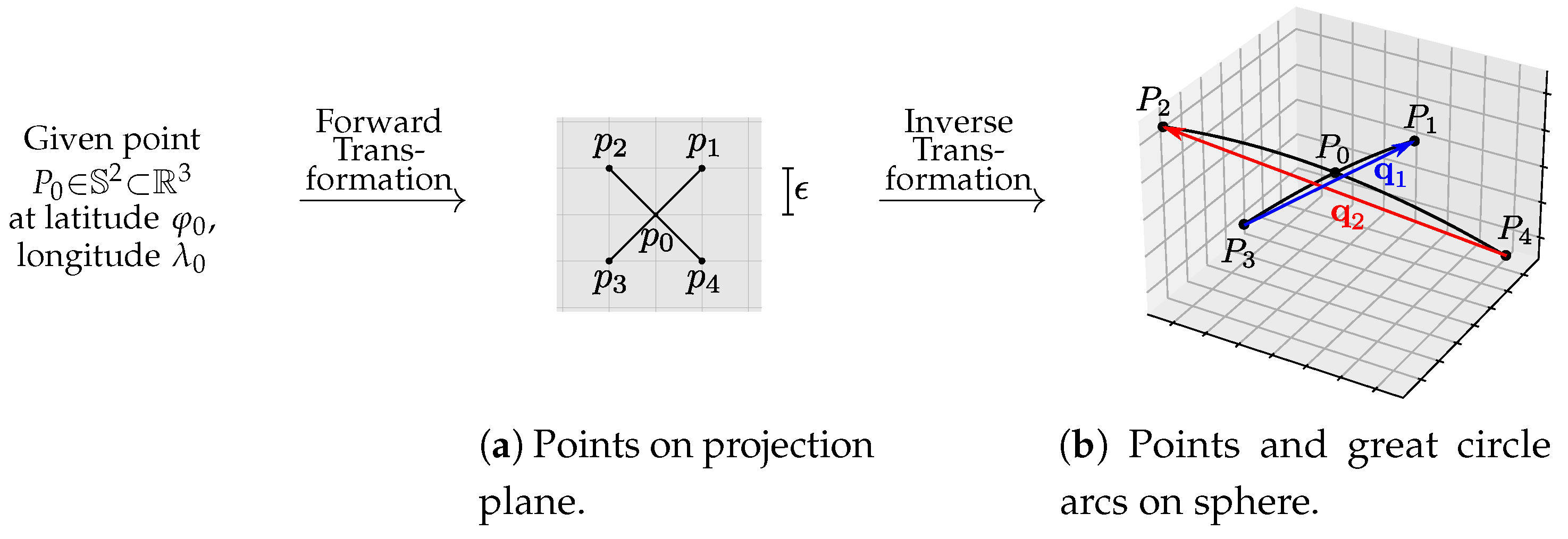
2.2. Gca-Based Metric

The averaged ratio metric between complementary profiles was introduced in [44], and uses small circle arcs on a sphere to evaluate the shape regularity of tessellation grids or map projections. Instead of small circle arcs, the simplified GCA-based metric [45] uses great circle arcs (see black arcs in Figure 1b) to calculate the area distortion $s_{gc}$ (see Equation (22)) and angular distortion ${\rho }_{gc}$ (see Equation (20)). Ref. [45] revealed that the metric ${\rho }_{gc}$ is a linear estimation of the differential-based metric ${\rho }_d$ (see Equation (21)).

The GCA-based metric can be calculated if the inverse equations of map projection are available. Given a map projection, the forward equations are assumed to be $x(\phi ,\lambda )$ and $y(\phi ,\lambda )$, and the inverse equations are assumed to be $\phi (x,y)$ and $\lambda (x,y)$, where $\phi$ and $\lambda$ are latitude and longitude coordinates, respectively, and x and y are planar coordinates on the given two-dimensional projection plane. Consider a point $P_0={\left(X_0,Y_0,Z_0\right)}^{\mathbf{T}}$ on the unit sphere ${\mathbb{S}}^2\subset {\mathbb{R}}^3$, the geographic coordinates of point $P_0$ can be calculated according to:

$$\left[\begin{array}{c}{\phi }_0\\ {\lambda }_0\end{array}\right]=\left[\begin{array}{c}arcsin{Z}_0\\ \arctan 2\left(Y_0,X_0\right)\end{array}\right],$$

(10)

where ${\phi }_0$ and ${\lambda }_0$ represent the latitude and longitude coordinates of point $P_0$, respectively.

The GCA-based metric can be calculated as:

First, calculate the coordinates of the projected point $p_0$ (see Figure 1a) on the projection plane by using the forward equations of map projection.

$$p_0=\left[\begin{array}{c}{x}_0\\ y_0\end{array}\right]=\left[\begin{array}{c}x\left({\phi }_0,{\lambda }_0\right)\\ y\left({\phi }_0,{\lambda }_0\right)\end{array}\right].$$

(11)

Next, calculate the four corner points (see Figure 1a) of an infinitesimal square on the projection plane as:

$$p_i=\left[\begin{array}{c}{x}_i\\ y_i\end{array}\right]=\left[\begin{array}{c}{x}_0\pm ϵ\\ y_0\pm ϵ\end{array}\right],$$

(12)

where $i=1,2,3,4$. We assume here that $p_1$ and $p_3$ are located on one diagonal of the square, $p_2$ and $p_4$ are located on the other diagonal of the square, and $ϵ$ is a sufficiently small value ($ϵ={10}^{-6}$ in this paper) representing half the length of the side of square. Points $p_i$, $i=1,2,3,4$, are located on the corners of a square, which is an undistorted quadrilateral on a plane. The diagonals of the square act as an orthogonal frame on the projection plane for the GCA-based metric. Inspired by the GCA-based method, the proposed FWD–GCA method (see Section 3) uses an orthogonal frame on the projection plane to establish metrics for evaluating the distortions of the map projections.

Now, let us consider the GCA-based method. We calculate the geographic coordinates ${\left({\phi }_i,{\lambda }_i\right)}^{\mathbf{T}}$ for each two-dimensional point $p_i$ using the inverse equations of the map projection as:

$$\left[\begin{array}{c}{\phi }_i\\ {\lambda }_i\end{array}\right]=\left[\begin{array}{c}\phi \left(x_i,y_i\right)\\ \lambda \left(x_i,y_i\right)\end{array}\right],$$

(13)

where $i=1,2,3,4$.

Subsequently, we calculate the Cartesian coordinates (i.e., the earth-centered, earth-fixed (ECEF) Cartesian coordinates) of the three-dimensional points $P_i$ (see Figure 1b) on the unit sphere ${\mathbb{S}}^2$ for each two-dimensional point $p_i$, $i=1,2,3,4$.

$$P_i=\left[\begin{array}{c}cos{\phi }_{i}cos{\lambda }_i\\ cos{\phi }_{i}sin{\lambda }_i\\ sin{\phi }_i\end{array}\right],$$

(14)

where $i=1,2,3,4$.

Now, prepare intermediate three-dimensional vectors ${\mathbf{q}}_i$ ($i=1,2$, see Figure 1b) and normalized three-dimensional vectors ${\widehat{\mathbf{q}}}_i$ ($i=1,2$) for the GCA-based metric, and calculate $r_i$ ($i=1,2$, see Figure 1b), which is the length of the great circle arc connecting points $P_i$ and $P_{i+2}$ on the sphere, where $i=1,2$.

$${\mathbf{q}}_i=P_i-P_{i+2},$$

(15)

$${\widehat{\mathbf{q}}}_i=\mathrm{normalize}\left({\mathbf{q}}_i\right),$$

(16)

$$r_i=2arcsin\frac{\left|{\mathbf{q}}_i\right|}{2},$$

(17)

where i (or $i$ for vectors ${\mathbf{q}}_i$ and ${\widehat{\mathbf{q}}}_i$) $=1,2$.

Next, calculate the length and angle components of the GCA-based metric.

$${\rho }_l=\frac{max\left(r_1,r_2\right)}{min\left(r_1,r_2\right)},$$

(18)

$${\rho }_{\alpha }=cot\left[\frac{1}{2}arccos\left|{\widehat{\mathbf{q}}}_1·{\widehat{\mathbf{q}}}_2\right|\right].$$

(19)

Finally, combine the above components as a GCA-based metric by the arithmetic mean.

$${\rho }_{gc}=\frac{1}{2}\left({\rho }_l+{\rho }_{\alpha }\right).$$

(20)

The GCA-based metric ${\rho }_{gc}$ has a strong (>0.988) linear correlation [44] to a differential-based shape regularity metric ${\rho }_d$.

$${\rho }_d=\frac{a}{b},$$

(21)

where the maximum and minimum linear scale factors a and b are calculated according to Equations (7) and (8).

The reciprocal of ${\rho }_d$ was at first defined as the metric of angular distortion, which is equal to $b/a$ [25,32,46]. The metric ${\rho }_d$ is then adopted in [44,45] to measure the shape distortion of the tessellation.

The area distortion is discussed in [45]. It is defined as the ratio between the area of the infinitesimal region on the projection plane and the area of the corresponding region on the sphere; $s_{gc}$ is introduced as an alternative to the differential-based areal scale factor s in Equation (9).

$$s_{gc}=\frac{8{ϵ}^2}{r_1{r}_{2}sin\left[arccos\left|{\widehat{\mathbf{q}}}_1·{\widehat{\mathbf{q}}}_2\right|\right]},$$

(22)

where $4{ϵ}^2$ is the area of infinitesimal square on the projection plane (see Figure 1a).

3. Forward Interpolated Version of Gca-Based Metric

The calculation of the GCA-based metric is dependent on $\phi (x,y)$ and $\lambda (x,y)$, the inverse equations of the map projection (see Equation (13)). To avoid the influence of inverse equations, the FWD–GCA metric, an interpolated version of the GCA-based metric, is introduced in this section. For a clear and intuitive comparison, Figure 2 summarize the principle of and difference among different methods. The GCA-based method generates four points, around the given point on the projection plane (${\mathbb{R}}^2$), while the proposed FWD–GCA-based method directly generates four points on the unit sphere ${\mathbb{S}}^2\subset {\mathbb{R}}^3$.

The FWD–GCA-based metric has two main steps. In Section 3.1, the sample points on the unit sphere ${\mathbb{S}}^2$ (on red lines in Figure 3a) are generated and converted to the projection plane (on red lines in Figure 3b). In Section 3.2, vector interpolation is applied to sample points on the projection plane to obtain orthogonal vectors (blue lines in Figure 3b), and the points on the orthogonal vectors (blue lines in Figure 3b) on the projection plane are converted to a sphere (denoted as ${\widehat{p}}_i$ on the blue lines in Figure 3c, $i=1,2,3,4$) to calculate the FWD–GCA metric. An implementation of the FWD–GCA metric on the unit sphere ${\mathbb{S}}^2$ in Julia is provided in Code S3 in the supplementary materials.

3.1. Spherical Sampling and Forward Projection

Given a three-dimensional point $P_0={\left(X_0,Y_0,Z_0\right)}^{\mathbf{T}}$ on the unit sphere ${\mathbb{S}}^2$, calculate the geographic coordinates ${\left({\phi }_0,{\lambda }_0\right)}^{\mathbf{T}}$ of point $P_0$ according to Equation (10) and the two-dimensional projection coordinates $p_0={\left(x_0,y_0\right)}^{\mathbf{T}}$ according to Equation (11).

The calculation for the FWD–GCA metric is as described below.

First, let E be a three-dimensional point on ${\mathbb{S}}^2$ and near $P_0$. For the ease of the calculation, E is offset along the z-axis (i.e., on the line between the North and South Poles, with positive values increasing northward) of ECEF Cartesian coordinates, whereas the singularity case is avoided (if $Z_0=\pm 1$) using a sign function of $Z_0$ (see Equation (24)).

$$E=\mathrm{normalize}\left(\left[\begin{array}{c}{X}_0\\ Y_0\\ Z_0-e\end{array}\right]\right),$$

(23)

$$e=\left\{\begin{array}{cc}\mathrm{sgn}\left(Z_0\right)ϵ& Z_0\ne 0\\ 1& Z_0=0\end{array}\right.,$$

(24)

where $ϵ$ is a sufficiently small value, and $ϵ={10}^{-6}$ in this paper.

Next, calculate four unit three-dimensional vectors as ${\mathbf{e}}_1=\mathrm{normalize}\left(E-P_0\right)$ and ${\mathbf{e}}_{i+1}={\mathbf{p}}_0\times {\mathbf{e}}_i$, where $i=1,2,3$; the three-dimensional vector ${\mathbf{p}}_0=P_0-O$ is the vector to $P_0$ in ${\mathbb{R}}^3$; and O denotes the origin of ${\mathbb{S}}^2$.

Now, calculate the four points (see black dots in Figure 3a) along the orthogonal axes (see red lines in Figure 3a) on ${\mathbb{S}}^2$ according to:

$$\left[\begin{array}{c}{X}_i\\ Y_i\\ Z_i\end{array}\right]=\mathrm{normalize}\left(P_0+{\mathbf{e}}_iϵ\right),$$

(25)

where i (or $i$ for vectors ${\mathbf{e}}_i$) $=1,2,3,4$, and $ϵ={10}^{-6}$ in this paper.

Convert the Cartesian coordinates of the sphere (Figure 3a) to the geographic coordinates ${\Phi }_i$ and ${\Lambda }_i$ using Equation (26); calculate four basis points $b_i$ on the projection plane (see Figure 3b) from ${\Phi }_i$ and ${\Lambda }_i$, $i=1,2,3,4$, using the forward equations of map projection (see Equation (27). The uppercase Greek letters $\Phi$ and $\Lambda$ with subscripts in Equations (26) and (27) are used to differentiate them with $\phi$ and $\lambda$ with subscripts in Equations (13) and (14). Figure 4 demonstrates more details and annotation than Figure 3b. In Figure 4, there are different cases of the relative positions of the points $b_i$ depending on the specific map projection and the positions of given geographic coordinates ${\phi }_0$ and ${\lambda }_0$.

$$\left[\begin{array}{c}{\Phi }_i\\ {\Lambda }_i\end{array}\right]=\left[\begin{array}{c}arcsin{Z}_i\\ \arctan 2\left(Y_i,X_i\right)\end{array}\right],$$

(26)

$$b_i=\left[\begin{array}{c}{x}_i\\ y_i\end{array}\right]=\left[\begin{array}{c}x\left({\Phi }_i,{\Lambda }_i\right)\\ y\left({\Phi }_i,{\Lambda }_i\right)\end{array}\right],$$

(27)

where $i=1,2,3,4$.

On the projection plane (see Figure 3b or Figure 4), calculate four two-dimensional basis vectors as:

$${\mathbf{b}}_i=b_i-p_0,$$

(28)

where i (or $i$ for vectors ${\mathbf{b}}_i$) $=1,2,3,4$.

In Figure 4, vectors ${\mathbf{b}}_i$ and ${\mathbf{b}}_{i+2}$ appear to be collinear, where $i=1,2$. However, this pair of vectors is not strictly collinear, as $ϵ$ in Equation (25) is not infinitely small.

Calculate the two normalized two-dimensional basis vectors ${\widehat{\mathbf{b}}}_i$ (marked as blue lines in Figure 4) as:

$${\widehat{\mathbf{b}}}_i=\mathrm{normalize}\left({\mathbf{b}}_i\right),$$

(29)

where $i=1,2$.

Additionally, calculate the angle $\alpha$ shown in Figure 4.

$$\alpha =\frac{1}{2}arccos\left({\widehat{\mathbf{b}}}_1·{\widehat{\mathbf{b}}}_2\right)-\frac{\pi }{4}.$$

(30)

Rotate ${\widehat{\mathbf{b}}}_1$ by angle $\alpha$ (or $-\alpha$) to obtain a normalized two-dimensional target vector $\widehat{\mathbf{t}}$ (see Figure 4) as:

$$\widehat{\mathbf{t}}=\left[\begin{array}{cc}cos\alpha & -sin\alpha \\ sin\alpha & cos\alpha \end{array}\right]{\widehat{\mathbf{b}}}_1.$$

(31)

3.2. Interpolation of Vectors on Sphere

Similar to sample points (see Figure 1a) on the projection plane coinciding with corners of a square in the GCA-based metric, the FWD–GCA-based metric needs to establish sample points on the projection plane to satisfy the relationship of orthogonal diagonals (see blue lines in Figure 3b). In Figure 4, red and yellow lines represent the candidate orthogonal frames for the FWD–GCA-based metric.

Interpolation based on the orthogonal frames is as described below. Firstly, establish and solve a set of equations (see Equations (32)–(35) or (40)–(43)) on the projection plane (see Figure 3b) to obtain the coefficients of interpolation depending on the sign of $\alpha$. Then, the coefficients are used to interpolate the point (see Equations (36)–(39) or (44)–(47)) on the sphere to obtain $P_i^{\prime }$, $i=1,2,3,4$ (see Figure 3c).

If $\alpha \ge 0$ (see Figure 4a), select ${\mathbf{b}}_1$ and ${\mathbf{b}}_2$ as the basis vector to solve Equations (32) and (33) and obtain interpolation coefficients for the two vectors (red lines in Figure 4a), and select ${\mathbf{b}}_3$ and ${\mathbf{b}}_4$ as the basis vector to solve Equations (34) and (35) and obtain interpolation coefficients for the other two vectors (yellow lines in Figure 4a).

$$ϵ\widehat{\mathbf{t}}=s_{11}{\mathbf{b}}_1+s_{21}{\mathbf{b}}_2,$$

(32)

$$\left[\begin{array}{cc}0& -1\\ 1& 0\end{array}\right]ϵ\widehat{\mathbf{t}}=s_{12}{\mathbf{b}}_1+s_{22}{\mathbf{b}}_2,$$

(33)

$$\left[\begin{array}{cc}-1& 0\\ 0& -1\end{array}\right]ϵ\widehat{\mathbf{t}}=s_{33}{\mathbf{b}}_3+s_{43}{\mathbf{b}}_4,$$

(34)

$$\left[\begin{array}{cc}0& 1\\ -1& 0\end{array}\right]ϵ\widehat{\mathbf{t}}=s_{34}{\mathbf{b}}_3+s_{44}{\mathbf{b}}_4.$$

(35)

The coefficient of interpolation $s_{ij}$ is calculated, where $i=1,2,3,4$ and $j=1,2,3,4$; we calculate points on sphere by vector interpolation as:

$$P_1^{\prime }=\mathrm{normalize}\left(P_0+ϵs_{11}{\mathbf{e}}_1+ϵs_{21}{\mathbf{e}}_2\right),$$

(36)

$$P_2^{\prime }=\mathrm{normalize}\left(P_0+ϵs_{12}{\mathbf{e}}_1+ϵs_{22}{\mathbf{e}}_2\right),$$

(37)

$$P_3^{\prime }=\mathrm{normalize}\left(P_0+ϵs_{33}{\mathbf{e}}_3+ϵs_{43}{\mathbf{e}}_4\right),$$

(38)

$$P_4^{\prime }=\mathrm{normalize}\left(P_0+ϵs_{34}{\mathbf{e}}_3+ϵs_{44}{\mathbf{e}}_4\right).$$

(39)

If $\alpha <0$ (Figure 4b), select ${\mathbf{b}}_1$ and ${\mathbf{b}}_4$ as the basis vectors to solve Equations (40) and (43), respectively, and obtain interpolation coefficients for the two vectors (red lines in Figure 4b). Similarly, select ${\mathbf{b}}_2$ and ${\mathbf{b}}_3$ as the basis vector to solve Equations (41) and (42) and obtain interpolation coefficients for the other two vectors (yellow lines in Figure 4b).

$$ϵ\widehat{\mathbf{t}}=s_{11}{\mathbf{b}}_1+s_{41}{\mathbf{b}}_4,$$

(40)

$$\left[\begin{array}{cc}0& -1\\ 1& 0\end{array}\right]ϵ\widehat{\mathbf{t}}=s_{22}{\mathbf{b}}_2+s_{32}{\mathbf{b}}_3,$$

(41)

$$\left[\begin{array}{cc}-1& 0\\ 0& -1\end{array}\right]ϵ\widehat{\mathbf{t}}=s_{23}{\mathbf{b}}_2+s_{33}{\mathbf{b}}_3,$$

(42)

$$\left[\begin{array}{cc}0& 1\\ -1& 0\end{array}\right]ϵ\widehat{\mathbf{t}}=s_{14}{\mathbf{b}}_1+s_{44}{\mathbf{b}}_4.$$

(43)

The coefficient of interpolation $s_{ij}$ is calculated, where $i=1,2,3,4$ and $j=1,2,3,4$; we calculate points on the sphere by vector interpolation as:

$$P_1^{\prime }=\mathrm{normalize}\left(P_0+ϵs_{11}{\mathbf{e}}_1+ϵs_{41}{\mathbf{e}}_4\right),$$

(44)

$$P_2^{\prime }=\mathrm{normalize}\left(P_0+ϵs_{22}{\mathbf{e}}_2+ϵs_{32}{\mathbf{e}}_3\right),$$

(45)

$$P_3^{\prime }=\mathrm{normalize}\left(P_0+ϵs_{23}{\mathbf{e}}_2+ϵs_{33}{\mathbf{e}}_3\right),$$

(46)

$$P_4^{\prime }=\mathrm{normalize}\left(P_0+ϵs_{14}{\mathbf{e}}_1+ϵs_{44}{\mathbf{e}}_4\right).$$

(47)

By substituting three-dimensional points $P_i^{\prime }$ (see Equations (36)–(39) or (44)–(47), and Figure 3c), $i=1,2,3,4$, into the right-hand side of Equation (15), we obtain three-dimensional vectors ${\mathbf{q}}_i$, $i=1,2$. Next, we obtain a forward version of the GCA-based metric (or FWD–GCA metric) according to Equations (16)–(20); it is denoted as ${\rho }_{fwd}$. Area distortion in the FWD–GCA metric can be obtained by rewriting Equation (22) as:

$$s_{fwd}=\frac{4{ϵ}^2}{r_1{r}_{2}sin\left[arccos\left|{\widehat{\mathbf{q}}}_1·{\widehat{\mathbf{q}}}_2\right|\right]},$$

(48)

where $ϵ$ is half the length of the diagonal of an infinitesimal square on the projection plane ($ϵ$ is half the length of side of an infinitesimal square in Equation (22)), and $2{ϵ}^2$ is the area of an infinitesimal square on the projection plane in Equation (48), while $4{ϵ}^2$ is the area of an infinitesimal square on the projection plane in Equation (22).

4. Regression Analysis

4.1. Linear Regression

According to the results in [44,45], the differential-based ${\rho }_d$ and GCA-based metric ${\rho }_{gc}$ are highly correlated (>0.988 for 14 non-conformal map projections [45]); hence, ${\rho }_{gc}$ can be approximately estimated from ${\rho }_d$, and vice versa using the linear regression model of ordinary least squares (OLS). That is,

$${\rho }_d\approx {\rho }_d^{gc}={\beta }_1^{gc}{\rho }_{gc}+{\beta }_0^{gc},$$

(49)

where ${\rho }_d^{gc}$ denotes a metric derived from metric ${\rho }_{gc}$; it is an approximation of metric ${\rho }_d$.

An example of metric distributions of ${\rho }_d$ and ${\rho }_{gc}$ is shown in Figure 5a,b with respective scalar bars for the Bonne projection with first standard parallel ${\phi }_1={30}^{\circ }$. The Pearson product-moment correlation coefficient (PPMCC) between ${\rho }_d$ and ${\rho }_{gc}$ for the Bonne projection is 0.9883, which is almost the worst result among the 14 non-conformal map projections in [45].

The black contours in Figure 5a are derived from the differential metric ${\rho }_d$, and the red contours in Figure 5b are derived from the metric ${\rho }_d^{gc}$ with coefficients ${\beta }_1^{gc}=2.25$ and ${\beta }_0^{gc}=-1.45$, respectively, which are generated via OLS-based regression. Based on the distortions and contours in Figure 5a,b, and the value of PPMCC, the metrics ${\rho }_d$ and ${\rho }_d^{gc}$ are found to be consistent, to a certain extent.

In Section 3, the proposed FWD–GCA metric is constructed from the GCA-based metric using the same mechanism of the GCA-based metric. As in the case of the GCA-based metric, we assume that the proposed FWD–GCA metric should also be a linear approximation of the differential metric ${\rho }_d$, i.e.,

$${\rho }_d\approx {\rho }_d^{fwd}={\beta }_1^{fwd}{\rho }_{fwd}+{\beta }_0^{fwd},$$

(50)

where ${\rho }_d^{fwd}$ denotes a metric derived from the metric ${\rho }_{fwd}$, and it should be an approximation to the metric ${\rho }_d$.

OLS-based regression can be applied to Equation (50) to obtain the coefficients ${\beta }_1^{fwd}$ and ${\beta }_0^{fwd}$. The distribution of the metric ${\rho }_{fwd}$ and contours of the metric ${\rho }_d^{fwd}$ are shown in Figure 5c for the Bonne projection with ${\phi }_1={30}^{\circ }$, where ${\beta }_1^{fwd}=2.00$ and ${\beta }_0^{fwd}=-1.08$. PPMCC between ${\rho }_d$ and ${\rho }_{fwd}$ is 0.9995, which means ${\rho }_d$ and ${\rho }_{fwd}$ are also highly correlated and have similar distributions for the Bonne projection.

4.2. Rational Function Regression

Now, let us consider the maximum angular distortion $\omega$ in Equation (6). Using Equations (6)–(8) and (21), we derive that:

$$\omega =2arcsin\frac{{\rho }_d-1}{{\rho }_d+1}.$$

(51)

As ${\rho }_d^{gc}$ and ${\rho }_d^{fwd}$ are approximations (see Equations (49) and (50)) of ${\rho }_d$ by OLS-based regression, we substitute the right-hand sides of Equations (49) and (50) into Equation (51); we can further assume that:

$$\omega \approx {\omega }_{gc}=2arcsin\frac{{\beta }_1^{gc}{\rho }_{gc}+{\beta }_0^{gc}-1}{{\beta }_1^{gc}{\rho }_{gc}+{\beta }_0^{gc}+1},$$

(52)

$$\omega \approx {\omega }_{fwd}=2arcsin\frac{{\beta }_1^{fwd}{\rho }_{fwd}+{\beta }_0^{fwd}-1}{{\beta }_1^{fwd}{\rho }_{fwd}+{\beta }_0^{fwd}+1},$$

(53)

where coefficients ${\beta }_0^{gc}$, ${\beta }_1^{gc}$, ${\beta }_0^{fwd}$, and ${\beta }_1^{fwd}$ are obtained by OLS-based regression.

As a comparison, metrics $\omega$, ${\omega }_{gc}$, and ${\omega }_{fwd}$ are calculated by linear regression with coefficients ${\beta }_1^{gc}=2.25$, ${\beta }_0^{gc}=-1.45$, ${\beta }_1^{fwd}=2.00$, and ${\beta }_0^{fwd}=-1.08$; the distributions and contours of $\omega$, ${\omega }_{gc}$, and ${\omega }_{fwd}$ are shown in Figure 6. All the above metrics of angular distortions have the same scale. In Section 5, we use the same scalar bar in Figure 6 to represent angular distortions of different map projections that are shown in Figures 9–16.

As shown in Equations (52) and (53), $\omega$ is represented by different forms of rational functions of GCA-based metric ${\rho }_{gc}$ or FWD–GCA-based metric ${\rho }_{fwd}$. Without the loss of generality, we rewrite Equations (52) and (53) and establish a general form for rational functions with degree one (or linear rational functions) for independent variables ${\rho }_{gc}$ or ${\rho }_{fwd}$ using unknown coefficients ${\delta }_i^{gc}$ or ${\delta }_i^{fwd}$, where $i=0,1,2$, as:

$$\omega \approx {\omega }_{gc}=2arcsin\frac{{\delta }_2^{gc}{\rho }_{gc}+{\delta }_1^{gc}}{{\delta }_0^{gc}{\rho }_{gc}+1},$$

(54)

$$\omega \approx {\omega }_{fwd}=2arcsin\frac{{\delta }_2^{fwd}{\rho }_{fwd}+{\delta }_1^{fwd}}{{\delta }_0^{fwd}{\rho }_{fwd}+1}.$$

(55)

4.3. Approach of Estimating Regression Coefficients

Equation (55) is a proposed equation to predict $\omega$ from the FWD–GCA-based metric with unknown coefficients. Therefore, we need to further establish an approach to estimate the value of coefficients, which can covers all different types of map projections, e.g., conformal, equal-area or compromise map projections.

Firstly, we would compare linear regression with the proposed rational function–based regression (see Section 5.2.1) to find out the distribution and characteristic of regression coefficients by considering as many map projections as possible. However, there are hundreds of map projections and their variants; therefore, one cannot enumerate as many of them as possible. That means it is impossible to make a regression for all innumerable existing map projections.

A practical approach is to use a limited number of randomly selected map projections to obtain individual regression coefficients ${\delta }_i^{fwd}$, $i=0,1,2$, for each map projection. Next, these individual regression coefficients are used to obtain synthesized coefficients based on the distribution and characteristic of regression coefficients. As the synthesized coefficients are obtained and validated, we can use Equation (55) to calculate ${\omega }_{fwd}$.

To further eliminate the effect of individual map projection, we can use certain groups of randomly selected map projections (see Section 5.2.2) to obtain individual regression coefficients, for each group of map projections. Then, we can obtain synthesized coefficients from these individual regression coefficients.

As only a limited numbers of map projections are used for regression, it is necessary to study the sensitivity (see Section 5.3.3) of regression coefficients ${\delta }_i^{fwd}$, $i=0,1,2$, yielding different sources of the selected map projections.

Next, we will estimate the coefficients of the above rational functions with degree one in Equation (55), as well as validate the accuracy of the above rational function–based regression method in Section 5.

5. Experiments and Validations of Metrics

5.1. Overview of Implementation and Experiments

More than 80 map projections for small-scale world maps in PROJ library [20] were evaluated in our study on a laptop with 64-bit quad-core of 1.9 GHz CPU, 16 GB memory, and 64-bit Manjaro Linux 21.0.3. Julia [47] is a modern, high-level, high-performance, and dynamic programming language. Differential metric (see Codes S1 and S2 in supplementary materials, and see Appendix A), GCA-based metric, and FWD–GCA metric (see Code S3) were implemented in Julia because of its speed and flexibility [47]. However, certain calculations, analyses, and plots were implemented in Python owing to its simplicity and usability. The versions of Julia and Python used were 1.6.1 and 3.9.4, respectively. Two additional Julia packages, Proj4.jl and ForwardDiff.jl [48], were employed in our implementation. Proj4.jl is a wrapper of PROJ library, which is a coordinate conversion tool. It is used to transform geographic coordinates to projection coordinates, and vice versa. The underlying version of PROJ used in Proj4.jl is 7.2.1. ForwardDiff.jl is used to calculate partial derivatives, which is used in differential methods for comparisons. A few additional Python packages, such as numpy, scipy, healpy, matplotlib, were also used in our experiments.

For all map projections we evaluated, we calculated the differential-based metrics s and ${\rho }_d$, and obtained $\omega$ by using Equation (51). We also calculated the GCA-based metrics $s_{gc}$ and ${\rho }_{gc}$, and the proposed FWD–GCA metrics $s_{fwd}$ and ${\rho }_{fwd}$. Then, ${\omega }_{gc}$ and ${\omega }_{fwd}$ were calculated for validating the approach of the proposed rational function–based regression. Approximately 200k sample points on the sphere were generated using healpy, a wrapper of HEALPix [35] algorithm, to evaluate the metrics $s_{gc}$, ${\rho }_{gc}$, ${\omega }_{gc}$, $s_{fwd}$, ${\rho }_{fwd}$, and ${\omega }_{fwd}$. Parameter $N_{side}=128$ was used in the HEALPix algorithm to generate approximately 200 k ($12\times N_{side}^2$) near-uniformly distributed sample points on the sphere for all map projections to be evaluated. All 200k sample points were shifted by 0.003 radians along the longitudinal direction to avoid $\lambda =\pm \pi$.

5.2. Distribution and Further Regression of Regression Coefficients

5.2.1. Distribution of Regression Coefficients

Firstly, we compared the linear regression and rational function–based regression between the differential metric and FWD–GCA-based metric for more than 80 map projections in the PROJ library.

Figure 7 demonstrates ${\beta }_0^{fwd}$ and ${\beta }_1^{fwd}$, the regression coefficients of linear regression (see Equation (50)) between ${\rho }_d$ and ${\rho }_{fwd}$, which are mentioned in Section 4.1. Although it appears that the regression coefficients ${\beta }_0^{fwd}$ and ${\beta }_1^{fwd}$ for most of the map projections in Figure 7 satisfy an appropriate linear relationship as the blue line, ${\beta }_0^{fwd}$ and ${\beta }_1^{fwd}$ have a fairly large difference for different map projections. It is difficult to select a pair of optimal regression coefficients ${\beta }_0^{fwd}$ and ${\beta }_1^{fwd}$ from Figure 7 for estimating ${\rho }_d$ by ${\rho }_{fwd}$ for all map projections.

As an alternative, rational function–based regression (see Equation (55)) discussed in Section 4.2 was applied to metrics $sin(\omega /2)$ and ${\rho }_{fwd}$. Regression coefficients ${\delta }_i^{fwd}$, $i=0,1,2$, for rational function–based regression are plotted in Figure 8 for each non-conformal map projection we studied. Ranges and correlations of coefficients ${\delta }_i^{fwd}$, $i=0,1,2$, are summarized in

Table 1. Summary of coefficients for rational function–based regression.

	All Non-Conformal Map Projections in Figure 8a	Most ${}^{†}$ Non-Cylindrical, Non-Conic, and Non-Azimuthal Projections in Figure 8b
range of ${\delta }_0^{fwd}$	$(1,\mathrm{approx}.8\times {10}^6)$	$(\mathrm{approx}.1.5,\mathrm{approx}.10.5)$
PPMCC (${\delta }_0^{fwd},{\delta }_1^{fwd}$)	−0.999999999999989	−0.9992
PPMCC (${\delta }_0^{fwd},{\delta }_2^{fwd}$)	0.999999999999992	0.9998

${}^{†}$ Rectangular polyconic (see letter “A” in Figure 8a) is a non-cylindrical, non-conic, and non-azimuthal projection, but it is not in Figure 8b.

.

Letters P to W in Figure 8b represent the same map projections as those marked as Letters A, B, and E-K in Figure 7 for comparison. It can be observed from Figure 7 and Figure 8b that regression coefficients of these map projections deviate from the blue line in Figure 7 but coincide to blue or red lines in Figure 8b. That means that rational function–based regression can produce coefficients satisfying a highly correlated linear relationship (see PPMCC in Table 1).

Although regression coefficients ${\delta }_i^{fwd}$ in Figure 8a,b have a fairly large range, $i=0,1,2$, we assumed that they should have an approximately linear relationship (see Equations (56) and (57)) with additional regression coefficients ${\gamma }_i$, $i=0,1,2,3$, according to the results shown in Figure 8.

$${\delta }_2^{fwd}\approx {\gamma }_3^{fwd}{\delta }_0^{fwd}+{\gamma }_2^{fwd},$$

(56)

$${\delta }_1^{fwd}\approx {\gamma }_1^{fwd}{\delta }_0^{fwd}+{\gamma }_0^{fwd}.$$

(57)

As linear relationships (see Equations (56) and (57)) are intuitively established for the rational function–based regression coefficients, we needed to further study the effectiveness of the above linear relationships as well to obtain definite regression coefficients ${\delta }_i^{fwd}$ (see Equation (55)), $i=0,1,2$, to estimate the maximum angular distortion $\omega$ using Equation (55) from the proposed the FWD–GCA metric ${\rho }_{fwd}$.

5.2.2. Regression Results of Random Selection of Map Projections

First, we studied a limited number of map projections whose rational function–based regression coefficient ${\delta }_0^{fwd}$ is less than 10 (see Figure 8b). We randomly selected 12 groups of 10 map projections from Figure 8b and used these map projections to calculate rational function–based regression coefficients ${\delta }_i^{fwd}$ (see Equation (55)), $i=0,1,2$, for each map projection; we then calculated ${\gamma }_i^{fwd}$, $i=0,1,2,3$, using linear regression (see Equations (56) and (57)), for each group of map projections.

The average of the rational function–based regression coefficient ${\delta }_0^{fwd}$ (i.e., ${\overline{\delta }}_0^{fwd}$), for 10 randomly selected map projections in each group, as well as linear regression results (i.e., ${\gamma }_i^{fwd}$, $i=0,1,2,3$) of rational function–based regression coefficients for each group of map projections are listed in Table S2 in supplementary materials for different selections of map projections. As a comparison, linear regression coefficients ${\beta }_0^{fwd}$ and ${\beta }_1^{fwd}$ between ${\rho }_d$ and ${\rho }_{fwd}$ (see Equation (50)) are also listed in Table S2.

Table 2. Summary of coefficients for 12 groups of randomly selected map projections.

Type of Regression	Coefficients	Range	Mean Value
Linear regression	${\beta }_0^{fwd}$	$(-6.27,-1.43)$	−2.25
	${\beta }_1^{fwd}$	$(2.35,5.40)$	2.84
Rational function–based regression	${\overline{\delta }}_0^{fwd}$	$(3.62,5.48)$	4.82
Linear regression for ${\delta }_0$ and ${\delta }_1$	${\gamma }_0^{fwd}$	$(-0.426,-0.150)$	−0.280
	${\gamma }_1^{fwd}$	$(-1.044,-0.976)$	−1.012
Linear regression for ${\delta }_0$ and ${\delta }_2$	${\gamma }_2^{fwd}$	$(0.281,0.408)$	0.349
	${\gamma }_3^{fwd}$	$(0.976,1.005)$	0.990

summarizes Table S2. Table 2 indicates that the ranges of ${\beta }_0^{fwd}$ and ${\beta }_1^{fwd}$ are consistent with the results in Figure 7, which implies regression coefficients of linear regression are varied for different selections of the map projections. Table 2 indicates that a lower deviation of coefficients ${\gamma }_i^{fwd}$, $i=0,1,2,3$, is obtained using rational function–based regression than ${\beta }_0^{fwd}$ and ${\beta }_1^{fwd}$, and they are obtained by linear regression.

5.3. Sensitivity of Regression Coefficients

5.3.1. Candidate of Regression Coefficients

As rational function–based regression (see Equation (55)) is established, we need definite coefficients (i.e., ${\delta }_i^{fwd}$ in Equation (55), $i=0,1,2$) for the regression. Now, let us select candidates for regression coefficients and study the sensitivity of the regression coefficients.

According to Table 2, we set regression coefficient ${\delta }_0^{fwd}$ as $4.82$ (the average of ${\overline{\delta }}_0^{fwd}$ in Table S2), and use ${\gamma }_i^{fwd}$, $i=0,1,2,3$, for each group of map projections, from Table S2, to calculate candidates of the other two regression coefficients ${\delta }_1^{fwd}$ and ${\delta }_2^{fwd}$ by using Equations (56) and (57). The candidates of regression coefficients are listed in

Table 3. Candidate coefficients for linear and rational function–based regression.

	Linear Regression			Rational Function–Based Regression
Group #	${\mathbf{\beta }}_0^{\mathbf{fwd}}$	${\mathbf{\beta }}_1^{\mathbf{fwd}}$	Used	${\mathbf{\delta }}_0^{\mathbf{fwd}}$	${\mathbf{\delta }}_1^{\mathbf{fwd}}$	${\mathbf{\delta }}_2^{\mathbf{fwd}}$	Used
Group 1				4.82	$-5.17$	5.12
Group 2				4.82	$-5.16$	5.12	✓
Group 3				4.82	$-5.16$	5.12
Group 4				4.82	$-5.14$	5.12
Group 5				4.82	$-5.18$	5.14	✓
Group 6				4.82	$-5.17$	5.13	✓
Group 7				4.82	$-5.15$	5.11	✓
Group 8	$-1.70$	2.48	✓	4.82	$-5.17$	5.12
Group 9	$-6.27$	5.40	✓	4.82	$-5.15$	5.11
Group 10				4.82	$-5.14$	5.11
Group 11				4.82	$-5.18$	5.13
Group 12				4.82	$-5.13$	5.11	✓
manual setting	$-1$	2	✓	4.82	$-5.13$	5.13	✓

. We also chose three pairs of ${\beta }_0^{fwd}$ and ${\beta }_1^{fwd}$ (see Table 3, two of them derived from Table S2 and one manually) for comparisons of linear regression. Rational function–based regression also uses a manual setting of coefficients.

Table 3 reveals that rational function–based regression produces the same or similar coefficients ${\delta }_i^{fwd}$, $i=0,1,2$, which are derived from ${\gamma }_i^{fwd}$ (see Table S2), $i=0,1,2,3$. Any values the same or similar of ${\delta }_i^{fwd}$, $i=0,1,2$ in Table 3, were not selected for further evaluation. Regression coefficients used for further sensitivity analyses of linear regression and rational function–based regression are marked in the fourth and last columns of Table 3, respectively.

5.3.2. Sensitivity of Regression Coefficients for Linear Regression

We used candidates of linear regression coefficients in Table 3 to calculate ${\omega }_{fwd}$ by using Equations (53) and (55). The distributions of ${\omega }_{fwd}$ calculated by different linear regression coefficients, and the corresponding contours of ${\omega }_{fwd}$ (in red) and $\omega$ (in black), are plotted in Fiugre Figure 9 for Putniṇš $P_4$, Winkel Tripel, Eckert II, and Collignon projections. For each map projection shown in Figure 9, we calculate ${\omega }_{fwd}$ and $\omega$ for approximately one million sample points on the projection plane. Contours of the metrics were also generated based on one million sample points.

Due to the symmetry of Putniṇš $P_4$, Winkel Tripel, and Eckert II projections, we only plotted a quarter area ($0\le \phi \le \pi /2$ and $0\le \lambda \le \pi$) on the projection plane in Figure 9a–c. The hemisphere of Collignon projection is plotted in Figure 9d due to the same reason.

PPMCC and root-mean-square error (RMSE) (see Equations (58) and (59)) were used to evaluate the correlation and error between the proposed FWD–GCA metric–based ${\omega }_{fwd}$. We calculated PPMCC and RMSE (see values in Figure 9, Figure 10, Figure 11, Figure 12 and Figure 13) by using approximately 200 k sample points on the sphere, which were generated using the HEALPix algorithm for the sake of consistency of evaluating different map projections.

$$\mathrm{PPMCC}\left(\omega ,{\omega }_{fwd}\right)=\frac{{\sum }_{i=1}^n\left[\left({\omega }^{\left(i\right)}-\overline{\omega }\right)\left({\omega }_{fwd}^{\left(i\right)}-{\overline{\omega }}_{fwd}\right)\right]}{\sqrt{{\sum }_{i=1}^n{\left({\omega }^{\left(i\right)}-\overline{\omega }\right)}^2}\sqrt{{\sum }_{i=1}^n{\left({\omega }_{fwd}^{\left(i\right)}-{\overline{\omega }}_{fwd}\right)}^2}},$$

(58)

$$\mathrm{RMSE}\left(\omega ,{\omega }_{fwd}\right)=\sqrt{\frac{1}{n}{\sum }_{i=1}^n{\left[{\omega }^{\left(i\right)}-{\omega }_{fwd}^{\left(i\right)}\right]}^2},$$

(59)

where n is the number of sample points.

According to the results in Figure 9, linear regression does not achieve a good estimation for all selections of ${\beta }_1^{fwd}$ and ${\beta }_0^{fwd}$, except using ${\beta }_1^{fwd}=2$ and ${\beta }_0^{fwd}=-1$.

5.3.3. Sensitivity of Regression Coefficients for Rational Function–Based Regression

Now, we study the sensitivity of regression coefficients ${\delta }_i^{fwd}$, $i=0,1,2$, for rational function–based regression. Distribution and contours based on the results of rational function–based regression are plotted using approximately one million sample points for Putniṇš $P_4$ (Figure 10), Winkel Tripel (Figure 11), Eckert II (Figure 12), and Collignon (Figure 13) projections, respectively.

According to Figure 10, Figure 11, Figure 12 and Figure 13, using the proposed FWD–GCA metric with rational function–based regression to estimate the maximum angular distortion $\omega$ is insensitive to the selections of reasonable regression coefficients ${\delta }_i^{fwd}$, $i=0,1,2$. By comparing rational function–based regression with multiple selections of regression coefficients and linear regression, we also noticed that rational function–based regression produces higher correlation (considering PPMCC metric and contours) and lower regression errors (considering RMSE metric).

It should be noted that contours are intuitive visual indicators of correlation, while PPMCC and RMSE are statistical indicators of correlation or error. From Figure 11 and Figure 13, Winkel Tripel projection has lower RMSE (about $1.{61}^{\circ }$ at best) between $\omega$ and ${\omega }_{fwd}$ than RMSE for Collignon projection (about $3.{21}^{\circ }$ at best); however, ${\omega }_{fwd}$ for Winkel Tripel projection has more visual deviations from the $\omega$ metric than deviations of the metrics for the Collignon projection.

5.4. Determination and Analysis of Regression Coefficients

5.4.1. Determination of Regression Coefficients

From the above comparison, there are different choices available for rational function–based regression coefficients ${\delta }_i^{fwd}$ (see Table 3), $i=0,1,2$. Furthermore, the proposed rational function–based regression is obviously insensitive to the selection of these reasonable regression coefficients. Now let us determine the rational function–based regression coefficients by considering conformal map projections whose $\omega =0$ or ${\rho }_d=1$.

When we let ${\omega }_{fwd}=0$ and ${\rho }_{fwd}=1$ in Equation (55) for conformal map projections, we can obtain that ${\delta }_2^{fwd}$ should be $-{\delta }_1^{fwd}$. Considering that the coefficients ${\delta }_i^{fwd}$ listed in Table 3 are insensitive, $i=0,1,2$, we selected ${\delta }_0^{fwd}=4.82$, ${\delta }_1^{fwd}=-5.13$, and ${\delta }_2^{fwd}=5.13$ as the preferred coefficients for regression.

5.4.2. Analysis of Cylindrical, Conic, and Azimuthal Projections

Next, we considered map projections whose coefficients ${\delta }_0^{fwd}\ge 10$ (or, precisely speaking, ${\delta }_0^{fwd}>{10}^6\gg 10$). Most such map projections are cylindrical, conic, and azimuthal, as shown in Figure 8a. Although the rational function–based regression produces very large regression coefficients for cylindrical, conic, and azimuthal map projections, the regression coefficients ${\delta }_i^{fwd}$, $i=0,1,2$, for cylindrical, conic, and azimuthal map projections satisfy the linear relationships between ${\delta }_2^{fwd}$ and ${\delta }_0^{fwd}$, and between ${\delta }_1^{fwd}$ and ${\delta }_0^{fwd}$ (see Figure 8a). As ${\delta }_0^{fwd}\gg 10$ and ${\delta }_0^{fwd}\approx -{\delta }_1^{fwd}\approx {\delta }_2^{fwd}$ (see Figure 8a), we can simplify Equation (55) and obtain that:

$$\omega \approx {\omega }_{fwd}=2arcsin\frac{{\rho }_{fwd}-1}{{\rho }_{fwd}}.$$

(60)

Considering Equations (51) and (60), we obtain that Equation (60) is equivalent to ${\rho }_d=2{\rho }_{fwd}-1$. Therefore, we can estimate ${\rho }_d$ from ${\rho }_{fwd}$ by using a linear function with ${\beta }_1=2$ and ${\beta }_0=-1$; then, we calculate $\omega$ using Equation (51) for cylindrical, conic, and azimuthal map projections.

Linear regression with coefficients ${\beta }_1=2$ and ${\beta }_0=-1$ was evaluated for non-cylindrical, non-conic, and non-azimuthal map projections in Figure 9 (see Section 5.3.2). However, for non-cylindrical, non-conic, and non-azimuthal map projections, rational function–based regression (see Figure 10, Figure 11, Figure 12 and Figure 13 in Section 5.3.3) is the preferred choice for calculating FWD–GCA-based ${\omega }_{fwd}$ (see Equation (55)).

5.4.3. Correlation and Error Analysis of Angular Distortion

Rational function–based regression (see Section 4.2) transforms the FWD–GCA-based metric ${\rho }_{fwd}$ (see Section 3) to ${\omega }_{fwd}$, an approximation to differential-based $\omega$; therefore, we calculated $\omega$, ${\omega }_{gc}$, and ${\omega }_{fwd}$ to evaluate the effectiveness of the angular distortion metric ${\omega }_{fwd}$ for all map projections we studied.

Tables S3–S6 in supplementary materials summarize PPMCC and RMSE between $\omega$ and ${\omega }_{gc}$ (or ${\omega }_{fwd}$) for more than 80 map projections that were investigated in this study.

In Table S3, cylindrical, conic, and azimuthal map projections used linear regression with coefficients ${\beta }_1^{fwd}=2$ and ${\beta }_0^{fwd}=-1$. In Table S4, non-cylindrical, non-conic, and non-azimuthal map projections use rational function–based regression with coefficients ${\delta }_0^{fwd}=4.82$, ${\delta }_1^{fwd}=-5.13$, and ${\delta }_2^{fwd}=5.13$. We used the same coefficients for the GCA-based metric (i.e., ${\beta }_i^{gc}={\beta }_i^{fwd}$, $i=0,1$, and ${\delta }_i^{gc}={\delta }_i^{fwd}$, $i=0,1,2$) for linear and rational function–based regression.

The GCA-based metric cannot be calculated for map projections without inverse equations. As PROJ library does not provide inverse equations for all map projections studied, Table S5 provides the FWD–GCA metric only for those map projections whose inverse equations are not provided by PROJ library.

Table S6 lists errors of angular distortion metrics for conformal map projections, where the maximum angular distortion is theoretically $0^{\circ }$.

From Tables S3–S6, it can be inferred that both GCA-based and FWD–GCA metrics have fairly similar results to differential metric. Moreover, the proposed FWD–GCA metric appears to be more consistent with differential-based metrics than GCA-based metrics, although there is no significant difference for both metrics. The results also imply that the proposed FWD–GCA metric is an alternative to the GCA-based metric and that it can be used to calculate the appropriation of the maximum angular distortion metric. The worst statistical cases of the FWD–GCA metric in Tables S3–S6 are Collignon (Figure 13), Tobler–Mercator (Figure 14b), Bacon Globular (Figure 15), Eckert II (Figure 12), Eckert IV, and general sinusoidal series ($m=2$, $n=3$) (Figure 14a) projections. Based on the worst cases of statistical indicators in Figure 12, Figure 13, Figure 14 and Figure 15, it can be deduced that the proposed FWD–GCA metric and rational function–based regression is effective for the angular distortion of map projections.

5.4.4. Correlation and Error Analysis of Area Distortion

Area distortion is also significant for map projections. We calculated PPMCC and RMSE between area distortion metrics s and $s_{gc}$ (see Equation (22), or $s_{fwd}$, see Equation (48)), and the results are listed in Tables S7–S9 in supplementary materials.

Metric $s_{gc}$ can be calculated for map projections with inverse equations; therefore, Table S7 provides the result for such types of map projections.

Metric $s_{gc}$ cannot be calculated for map projections without inverse equations; therefore, metric $s_{fwd}$ for these map projections was calculated and evaluated (see Table S8).

There are many equal area map projections; theoretically, s is equal to 1 for them. We calculated RMSE between metrics for these map projections (see Table S9).

Compared to the angular distortion, the proposed forward version of the area distortion $s_{fwd}$ (see Equation (48)) is highly correlated with the differential-based metric s (see Equation (9), or, precisely speaking, $s_{fwd}$ is almost the same as s).

6. Evaluation and Comparison of Map Projections

As the proposed metric and regression method proved to be valid for distortion evaluation for map projections, we used that metric to compare certain map projections. Figure 15 and Figure 16 demonstrate this comparison. Due to the symmetry, only a quarter area ($0\le \phi \le \pi /2$ and $0\le \lambda \le \pi$) on the projection plane is plotted in Figure 15 and Figure 16. The scalar bar of area distortion is plotted in the right side of Figure 15. Yellow represents no area distortion ($s=1$), warm colors represent deflation of area ($s<1$), and cool colors represent inflation of area ($s>1$).

Certain map projections have the same or similar shapes, but their distortions are dissimilar. A comparison of the distortions of these similar map projections is beneficial in choosing the appropriate map projections for specific applications and controlling distortions under reasonable ranges.

As shown in Figure 15, the Hammer and Aitoff projections have the same shape (2:1 ellipses). From Figure 15a, we can observe that the Aitoff projection has a lower angular distortion than the Hammer projection in high latitude areas. However, the Hammer projection (equal area, not provided in Figure 15a) has a lower area distortion than the Aitoff projection.

From Figure 15b, we observe that the Apian Globular I and Ortelius oval map projections have similar distortions but the shapes of these two map projections are slightly different. In contrast, while Bacon Globular and Ortelius oval projections have very similar shapes, the distortions of these two map projections are obviously different.

It should also be noted that the PROJ library does not provide inverse equations for map projections that are listed in Tables S5 and S8. This means that it fails to calculate GCA-based metrics for these two map projections. In addition, calculating distributions and contours, as shown in Figure 15b and Figure 16, is also inconvenient because one cannot directly establish approximately one million sample points on a projection plane, as shown in the map projections of Figure 9, Figure 10, Figure 11, Figure 12, Figure 13 and Figure 14. As an alternative, we used the HEALPix algorithm to generate approximately three million sample points ($12\times N_{side}^2$, where $N_{side}=512$) on sphere ${\mathbb{S}}^2$, and calculated the metrics ${\rho }_d$, $\omega$, s, ${\rho }_{fwd}$, ${\omega }_{fwd}$, and $s_{fwd}$ for these three million sample points. Then, we used cubic interpolation for the unstructured 2-D grid (i.e., on the two-dimensional projection plane) to calculate the metrics and contours (see Figure 15b and Figure 16) for approximately one million sample points on the projection plane.

7. Discussion and Conclusions

We constructed and validated a forward version of the great circle arcs–based (or FWD–GCA-based) metrics ${\rho }_{fwd}$ and $s_{fwd}$ for evaluating angular and area distortion of map projections. The proposed metric is uniform irrespective of whether inverse equations for map projections exist or not, or the type of forward equations used (e.g., explicit or implicit). Although the differential-based metric also has unified formulae, the differential calculation may be complicated for certain map projections, and Newton–Raphson may be needed for some map projections with implicit equations. The use of ${\rho }_{fwd}$ avoids manual or auto calculation of the derivation, especially for map projections with singularity points of derivation, or implicit, interrupted, or non-differentiable forms of forward equations.

Compared to the differential-based metric and GCA-based metric, this study simplifies the process of calculating the distortions in map projections and expands the evaluation scope of map projections that can be evaluated by distortion metrics. The FWD–GCA-based metric is not dependent on inverse equations of map projections, and the only prerequisite for it is the existence of forward equations of the map projections. This implies that the proposed metric ${\rho }_{fwd}$ has a higher feasibility and usability than the differential metric $\omega$.

Using rational function–based regression and linear regression, we could further estimate the maximum angular distortion ${\omega }_{fwd}$. Experimental results reveal that ${\omega }_{fwd}$, which is derived from ${\rho }_{fwd}$, is a good approximation to $\omega$. For non-cylindrical, non-conic, non-azimuthal, and non-conformal map projections studied in the experiments, the average errors of angular distortion were less than $1.{778}^{\circ }$ (i.e., the average of values in the last column in Tables S4 and S5 in supplementary materials) by employing rational function–based regression with coefficients ${\delta }_0^{fwd}=4.82$, ${\delta }_1^{fwd}=-5.13$, and ${\delta }_2^{fwd}=5.13$. While the average errors of angular distortion were less than $0.{00032}^{\circ }$ (i.e., the average of values in the last column in Tables S3 and S6 in supplementary materials) for cylindrical, conic, and azimuthal map projections by employing linear regression with coefficients $bet{a}_1^{fwd}=2$ and ${\beta }_0^{fwd}=-1$, and for conformal map projections, by employing rational function–based regression.

In addition, there are still certain noticeable errors between FWD–GCA-based metric ${\omega }_{fwd}$ and differential-based metric $\omega$ in areas of lower distortions. However, for areas of higher distortions, which are of significant interest to researchers or mapmakers, ${\omega }_{fwd}$ is more consistent with $\omega$.

A limitation of the proposed metric is the boundary problem on the projection plane. When $\lambda$ approaches $\pm \pi$, four points on the sphere (see Figure 3a) may be located on either side of the prime meridian for several map projections, and the corresponding four points on the projection plane (see $p_i$ in Figure 3b, where $i=1,2,3,4$) may be separated far away due to the projection. The above situation may incur errors in the process of vector interpolation (see Figure 3b,c). Therefore, $\pm \pi$ should be avoided for $\lambda$. In our implementation, approximately 200k sample points, generated by HEALPix, were shifted by 0.003 radian along the longitudinal direction. To calculate the metric of a sample point when $\lambda =\pm \pi$ for several map projections, the sample point can also be slightly shifted (e.g., by $1\times {10}^{-5}$ radian) along the longitudinal direction for an approximate calculation.

Additionally, the existing PROJ library provides coordinate transformation functions; and the proposed FWD–GCA metric employs PROJ to evaluate the distortion of map projections. However, the proposed FWD–GCA metric is not restricted to map projections provided in PROJ library; we can evaluate any map projections with forward equations by the FWD–GCA metric. As PROJ library provides convenience for the calculation of distortions, a practical implication of this study is the use of existing libraries. Apart from PROJ, there are several open or closed source softwares, such as NASA’s G.Projector and Mapthematics LLC’s Geocart. These mapping softwares support a greater number of map projections and provide transformation functions for raster images; however, they do not provide explicit mathematical functions for coordinate transformations. In the future, we will investigate practical numerical approaches to evaluate distortions based on raster images and further improve the differential-independent metric proposed in this study.

References

1. ICA Executive Committee. A Strategic Plan for the International Cartographic Association 2003–2011. Available online: https://icaci.org/files/documents/reference_docs/ICA_Strategic_Plan_2003-2011.pdf (accessed on 26 September 2021).
2. Snyder, J.P. Map Projections: A Working Manual; USGS Publications Warehouse: Washington, DC, USA, 1987; Available online: https://books.google.com/books?id=nPdOAAAAMAAJ (accessed on 10 September 2021).
3. McDonnell, P.W. Map projections. In The Surveying Handbook, 2nd ed.; Springer: Berlin/Heidelberg, Germany, 1995; pp. 435–453. [Google Scholar]
4. Hargitai, H.; Wang, J.; Stooke, P.J.; Karachevtseva, I.; Kereszturi, Á.; Gede, M. Map projections in planetary cartography. In Choosing a Map Projection; Springer: Berlin/Heidelberg, Germany, 2017; pp. 177–202. [Google Scholar] [CrossRef]
5. Iwai, Y.; Murayama, Y. Geographical analysis on the projection and distortion of INŌ’s Tokyo map in 1817. ISPRS Int. J. Geo-Inf. 2019, 8, 452. [Google Scholar] [CrossRef] [Green Version]
6. Roşca, D.; Plonka, G. Uniform spherical grids via equal area projection from the cube to the sphere. J. Comput. Appl. Math. 2011, 236, 1033–1041. [Google Scholar] [CrossRef] [Green Version]
7. Jenny, B.; Šavrič, B.; Patterson, T. A compromise aspect-adaptive cylindrical projection for world maps. Int. J. Geogr. Inf. Sci. 2015, 29, 935–952. [Google Scholar] [CrossRef]
8. Holhoş, A.; Roşca, D. Area preserving maps and volume preserving maps between a class of polyhedrons and a sphere. Adv. Comput. Math. 2017, 43, 677–697. [Google Scholar] [CrossRef] [Green Version]
9. Strebe, D. A bevy of area-preserving transforms for map projection designers. Cartogr. Geogr. Inf. Sci. 2019, 46, 260–276. [Google Scholar] [CrossRef]
10. Šavrič, B.; Jenny, B. A new pseudocylindrical equal-area projection for adaptive composite map projections. Int. J. Geogr. Inf. Sci. 2014, 28, 2373–2389. [Google Scholar] [CrossRef]
11. Strebe, D. An adaptable equal-area pseudoconic map projection. Cartogr. Geogr. Inf. Sci. 2016, 43, 338–345. [Google Scholar] [CrossRef]
12. Strebe, D. An efficient technique for creating a continuum of equal-area map projections. Cartogr. Geogr. Inf. Sci. 2018, 45, 529–538. [Google Scholar] [CrossRef]
13. Jenny, B.; Patterson, T. Blending world map projections with Flex Projector. Cartogr. Geogr. Inf. Sci. 2013, 40, 289–296. [Google Scholar] [CrossRef]
14. Jenny, B.; Šavrič, B. Combining world map projections. In Choosing a Map Projection; Springer: Berlin/Heidelberg, Germany, 2017; pp. 203–211. [Google Scholar] [CrossRef]
15. Jenny, B.; Šavrič, B. Enhancing adaptive composite map projections: Wagner transformation between the Lambert azimuthal and the transverse cylindrical equal-area projections. Cartogr. Geogr. Inf. Sci. 2018, 45, 456–463. [Google Scholar] [CrossRef]
16. Canters, F. Small-Scale Map Projection Design; CRC Press: Boca Raton, FL, USA, 2002. [Google Scholar]
17. Šavrič, B.; Jenny, B.; Patterson, T.; Petrovič, D.; Hurni, L. A polynomial equation for the Natural Earth projection. Cartogr. Geogr. Inf. Sci. 2011, 38, 363–372. [Google Scholar] [CrossRef]
18. Baselga, S. TestGrids: Evaluating and optimizing map projections. J. Surv. Eng. 2019, 145, 04019004. [Google Scholar] [CrossRef]
19. Kunimune, J.H. Minimum-error world map projections defined by polydimensional meshes. Int. J. Cartogr. 2021, 21, 78–99. [Google Scholar] [CrossRef]
20. Evenden, G.I. libproj4: A Comprehensive Library of Cartographic Projection Functions (Preliminary Draft); Technical Report; Falmouth, MA, USA, 2008; Available online: http://citeseerx.ist.psu.edu/viewdoc/summary?doi=10.1.1.620.4554 (accessed on 26 September 2021).
21. Kessler, F.C.; Battersby, S.E.; Finn, M.P.; Clarke, K.C. Map projections and the Internet. In Choosing a Map Projection; Springer: Berlin/Heidelberg, Germany, 2017; pp. 117–148. [Google Scholar] [CrossRef]
22. Robinson, A.H. The Committee on Map Projections. Which map is best? In Choosing a Map Projection; Springer: Berlin/Heidelberg, Germany, 2017; pp. 1–14. [Google Scholar] [CrossRef]
23. Robinson, A.H. The Committee on Map Projections. Choosing a world map. In Choosing a Map Projection; Springer: Berlin/Heidelberg, Germany, 2017; pp. 15–48. [Google Scholar] [CrossRef]
24. Kerkovits, K. Comparing finite and infinitesimal map distortion measures. Int. J. Cartogr. 2019, 5, 3–22. [Google Scholar] [CrossRef]
25. Kerkovits, K. A statistical reinterpretation and assessment of criteria used for measuring map projection distortion. Cartogr. Geogr. Inf. Sci. 2020, 47, 481–491. [Google Scholar] [CrossRef]
26. Kessler, F.C.; Battersby, S.E. Working with Map Projections: A Guide to Their Selection; CRC Press: Boca Raton, FL, USA, 2019. [Google Scholar]
27. Gosling, P.C.; Symeonakis, E. Automated map projection selection for GIS. Cartogr. Geogr. Inf. Sci. 2020, 47, 261–276. [Google Scholar] [CrossRef]
28. Tissot, A. Mémoire sur la Représentation des Surfaces et les Projections des Cartes Géographiques; Gauthier-Villars: Paris, France, 1881. [Google Scholar]
29. Papadopoulos, A. Nicolas-Auguste Tissot: A link between cartography and quasiconformal theory. Arch. Hist. Exact Sci. 2017, 71, 319–336. [Google Scholar] [CrossRef] [Green Version]
30. Laskowski, P.H. The traditional and modern look at Tissot’s Indicatrix. Am. Cartogr. 1989, 16, 123–133. [Google Scholar] [CrossRef]
31. Goldberg, D.M.; Gott, J.R., III. Flexion and skewness in map projections of the earth. Cartogr. Int. J. Geogr. Inf. Geovis. 2007, 42, 297–318. [Google Scholar] [CrossRef] [Green Version]
32. Kerkovits, K. Calculation and visualization of flexion and skewness. Kartogr. Geoinf. 2018, 17, 32–45. [Google Scholar] [CrossRef] [Green Version]
33. Capek, R. Which is the best projection for the world map? In Proceedings of the 20th International Cartographic Conference, Beijing, China, 6–10 August 2001; Volume 5, pp. 3084–3093. Available online: http://citeseerx.ist.psu.edu/viewdoc/summary?doi=10.1.1.468.2289 (accessed on 26 September 2021).
34. Šavrič, B.; Patterson, T.; Jenny, B. The Equal Earth map projection. Int. J. Geogr. Inf. Sci. 2019, 33, 454–465. [Google Scholar] [CrossRef]
35. Górski, K.M.; Hivon, E.; Banday, A.J.; Wandelt, B.D.; Hansen, F.K.; Reinecke, M.; Bartelmann, M. HEALPix: A framework for high-resolution discretization and fast analysis of data distributed on the sphere. Astrophys. J. 2005, 622, 759. [Google Scholar] [CrossRef]
36. Gao, Y.; Du, Z.; Xu, W.; Li, M.; Dong, W. HEALPix-IA: A global registration algorithm for initial alignment. Sensors 2019, 19, 427. [Google Scholar] [CrossRef] [Green Version]
37. Robinson, A.H. The Committee on Map Projections. Matching the map projection to the need. In Choosing a Map Projection; Springer: Berlin/Heidelberg, Germany, 2017; pp. 49–116. [Google Scholar] [CrossRef]
38. Snyder, J.P. An equal-area map projection for polyhedral globes. Cartogr. Int. J. Geogr. Inf. Geovis. 1992, 29, 10–21. [Google Scholar] [CrossRef]
39. Robinson, A.H. A new map projection: Its development and characteristics. Int. Yearb. Cartogr. 1974, 14, 145–155. [Google Scholar]
40. Solanilla, L.; Oostra, A.; Yáñez, J.P. Peirce Quincuncial projection. Rev. Integr. 2016, 34, 23–38. [Google Scholar] [CrossRef] [Green Version]
41. Christensen, A.H. The Chamberlin Trimetric projection. Cartogr. Geogr. Inf. Syst. 1992, 19, 88–100. [Google Scholar] [CrossRef]
42. White, D.; Kimerling, A.J.; Sahr, K.; Song, L. Comparing area and shape distortion on polyhedral-based recursive partitions of the sphere. Int. J. Geogr. Inf. Sci. 1998, 12, 805–827. [Google Scholar] [CrossRef]
43. Sahr, K.; White, D.; Kimerling, A.J. Geodesic discrete global grid systems. Cartogr. Geogr. Inf. Sci. 2003, 30, 121–134. [Google Scholar] [CrossRef] [Green Version]
44. Yan, J.; Song, X.; Gong, G. Averaged ratio between complementary profiles for evaluating shape distortions of map projections and spherical hierarchical tessellations. Comput. Geosci. 2016, 87, 41–55. [Google Scholar] [CrossRef]
45. Yan, J.; Yang, X.; Li, N.; Gong, G. Spherical great circle arcs based indicators for evaluating distortions of map projections. Acta Geod. Cartogr. Sin. 2020, 49, 711–723. [Google Scholar] [CrossRef]
46. Bayeva, Y.Y. Kriterii otsenki dostoinstva kartograficheskikh proyektsiy ispolzuemykh dlya sostavleniya kart mira. Geod. Aerofotosyomka 1987, 3, 109–112. [Google Scholar]
47. Bezanson, J.; Edelman, A.; Karpinski, S.; Shah, V.B. Julia: A fresh approach to numerical computing. SIAM Rev. 2017, 59, 65–98. [Google Scholar] [CrossRef] [Green Version]
48. Revels, J.; Lubin, M.; Papamarkou, T. Forward-mode automatic differentiation in Julia. arXiv 2016, arXiv:1607.07892. [Google Scholar]
Figure 1. Schematic diagram of sample points and spherical arcs for GCA-based metrics. (a) Points on projection plane; (b) Points and great circle arcs on sphere.
Ijgi 10 00649 g001
Figure 2. Comparison of differential, GCA-based, and FWD–GCA-based methods.
Ijgi 10 00649 g002
Figure 3. Schematic diagram of sampling and interpolation for the proposed FWD–GCA-based metrics.
Ijgi 10 00649 g003
Figure 4. Two-dimensional points and vectors on the projection plane under the different conditions of α . (a) α 0 ; (b) α < 0 .
Ijgi 10 00649 g004
Figure 5. Distribution and contours of the differential-based, GCA-based, and FWD–GCA metrics for the Bonne projection.
Ijgi 10 00649 g005
Figure 6. Distribution and contours of the maximum angular distortion for the Bonne projection by linear regression.
Ijgi 10 00649 g006
Figure 7. Regression coefficients (in dots or stars) of linear regression for non-conformal map projections. Capital letters represent Tobler-Mercator (A), Bonne ( φ 1 = 30 ) (B), Lambert equal area conic (C), Albers equal area ( φ 1 = 20 , φ 2 = 60 ) (D), Nell (E), Hatano asymmetrical equal area (F), Eckert II (G), general sinusoidal series ( m = 2 , n = 3 ) (H), Urmaev FPS (I), Urmaev V (J), and Lambert azimuthal equal area (K) projections.
Ijgi 10 00649 g007
Figure 8. Regression coefficients δ i f w d (in black, red, or blue dots), i = 0 , 1 , 2 , of rational function–based regression for non-conformal map projections. Capital letters represent rectangular polyconic (A), Lambert equal area conic (B), Patterson cylindrical (C), compact Miller (D), Miller cylindrical (E), Gall stereographic (F), Lambert azimuthal equal area (G), Plate Carrée (H), Albers equal area ( φ 1 = 20 , φ 2 = 60 ) (I), azimuthal equidistant (J), Lambert conformal conic alternative ( φ 0 = 40 ) (K), equidistant conic ( φ 1 = 20 , φ 2 = 60 ) (L), equal area cylindrical ( φ t s = 0 ) (M), Gall isographic (N), equal area cylindrical ( φ t s = 45 ) (O), Urmaev V (P), Eckert II (Q), general sinusoidal series ( m = 2 , n = 3 ) (R), Urmaev FPS (S), Hatano asymmetrical equal area (T), Nell (U), Tobler–Mercator (V), Bonne ( φ 1 = 30 ) (W), Collignon (X), and Bacon Globular (Y) projections.
Ijgi 10 00649 g008
Figure 9. Distribution and contours (in red) of FWD–GCA metric based on linear regression with different regression coefficients.
Ijgi 10 00649 g009
Figure 10. Distribution and contours (in red) of FWD–GCA metric for evaluating Putniṇš P 4 (Craster Parabolic) projection using rational function–based regression with different regression coefficients.
Ijgi 10 00649 g010
Figure 11. Distribution and contours (in red) of FWD–GCA metric for evaluating Winkel Tripel projection using rational function–based regression with different regression coefficients.
Ijgi 10 00649 g011
Figure 12. Distribution and contours (in red) of FWD–GCA metric for evaluating Eckert II projection using rational function–based regression with different regression coefficients.
Ijgi 10 00649 g012
Figure 13. Distribution and contours (in red) of FWD–GCA metric for evaluating Collignon projection using rational function–based regression with different regression coefficients.
Ijgi 10 00649 g013
Figure 14. Distribution and contours (in red) of FWD–GCA metric for evaluating angular distortions of map projections whose errors are statistically large.
Ijgi 10 00649 g014
Figure 15. Comparison of distributions and contours of the FWD–GCA metric for evaluating similar map projections.
Ijgi 10 00649 g015
Figure 16. Distributions and contours (in red) of the FWD–GCA-based angular metric for evaluating more map projections without inverse equations.
Ijgi 10 00649 g016