Spatial Relations Using High Level Concepts

Abstract

Existing models of spatial relations do not consider that different concepts exist on different levels in a hierarchy and in turn that the spatial relations in a given scene area function of the specific concepts considered. One approach to determining the existence of a particular spatial relation is to compute the corresponding high level concepts explicitly using map generalization before inferring the existence of the spatial relation in question. We explore this idea through the development of a model of the spatial relation “enters” that may exist between a road and a housing estate.

1. Introduction

Murphy [1] defines a concept as the mental representation corresponding to a category. A house is a concept defined by the Merriam-Webster dictionary as a building that serves as living quarters for one or a few families. A housing estate is a higher level concept defined by the Merriam-Webster dictionary as a group of individual dwellings or apartment houses typically of similar design that are usually built and sold or leased by one management. In this work we use the term housing estate to refer to a specific instance of this concept. That is, a housing estate which consists of only detached, semi-detached and terraced residential houses. Housing estates are a commonly occurring structure in many European countries such as Ireland. Most housing estates have one or more corresponding roads which provide access to the houses in questions and are called the access roads for the estate in question. For example consider the scene in Figure 1 which depicts the housing estate Tudor Lawns located in Foxrock Dublin. The grey road corresponds to the access road for the housing estate in question. For a given scene containing a housing estate and a set of roads, the access road for the estate in question may not be stored explicitly but can be derived from implicit information in the scene [2]. For example a visual inspection of Figure 1 suggests that the grey road is the access for the housing estate in question. Deriving certain forms of implicit information from spatial data can be considered a problem of determining the existence of spatial relations. For example the verb enter is commonly used to describe the spatial relation which exists between a housing estate and its corresponding access road. Therefore we say that the grey road enters the housing estate in Figure 1.

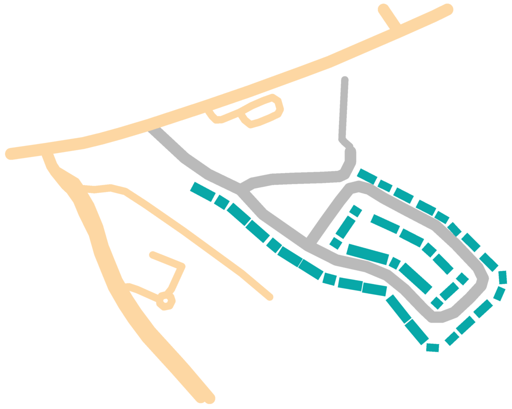
Figure 1. A set of polygons corresponding to houses in a housing estate and a number of lines corresponding to roads are represented. The grey line represents the access road for the housing estate in question. Data taken from OpenStreetMap.

Our cognitive capacity to infer this spatial relation of enters is a consequence of our ability to represent the spatial information using high level concepts before inferring the existence of the spatial relation in question. That is, representing the individual houses as a higher level housing estate concept before inferring the existence of the spatial relation enters. Despite the huge body of work on modeling spatial relations all existing models do not consider that different concepts may exist on different levels in a hierarchy. A number of authors have previously considered the effect splitting or merging of objects has on spatial relations [3,4,5]. However these works do not consider that different concepts exist on different levels in a hierarchy and in turn that the spatial relations in a given scene are a function of the specific concepts considered. In this work we propose that one may determine the existence of a spatial relation by computing the corresponding high level concepts explicitly using map generalization before inferring the existence of the spatial relation in question. We explore this idea through the development of a model of the spatial relation enters which may exist between a road and a housing estate.

The layout of this paper is as follows. In Section 2 we review related works. In Section 3 we present a model of the spatial relation enters. Section 4 evaluates this model and demonstrates it to be a useful tool for classifying housing estate access roads. Finally in Section 5 we draw conclusions and discuss possible future research directions.

2. Related Work

This section is divided into three parts. In Section 2.1 we briefly review existing methods for deriving implicit information from maps with a specific focus on information relating to buildings. In Section 2.2 we review existing models of spatial relations. Section 2.3 discusses the topic of map generalization.

2.1. Implicit Spatial Information

Implicit information derived from spatial data can be used to support many applications such as map generalisation (where this process is known as data enrichment) [6,7], improving the quality of user generated spatial data [8], matching spatial datasets [9] and updating data [10]. Walter and Luo [2] provide a classification of the different forms of implicit information that can be derived from spatial data. These include map type, single objects, complex objects and regions.

As stated by Luscher et al. [11] building objects are rarely attributed richly in spatial datasets. Consequently many authors have proposed methods for deriving implicit information relating to buildings. Regnault [12], Yan et al. [13], Steinhauer et al. [14] and Qi and Li [15] all proposed methods for the grouping of buildings. Zhang et al. [16] proposed a categorization of building patterns which includes collinear, curvilinear, align-along-road, grid-like and unstructured. The detection of collinear building patterns has been extensively studied [17,18]. Zhang et al. [16] proposed algorithms for detecting align-along-road and unstructured building patterns. Luscher et al. [19] demonstrated that higher level semantics, such as terraced house, can be derived from building alignments and other criteria. Haunert [20] proposed a methodology for detecting symmetries in building footprints.

2.2. Spatial Relations

A spatial relation is a means of modeling a particular property of the spatial relationship which exists between two or more objects. Spatial relations may be categorized as topological, metric and order relations [21]. Topological relations model properties which are invariant under consistent topological transformations such as rotation, translation and scaling [22]. Metric relations model properties concerning distance and direction. Order relations model properties concerning the partial and total order of objects as described by prepositions such as in front of, behind, above, and below [23]. Many spatial relations cannot be classified as exclusively topological, metric or order. Such relations include the align-along-road relation existing between a set of buildings and a road. A number of authors have considered the effect splitting and merging objects has on topological relations [3,4,5].

Research on the topic of spatial relations is motivated by a broad spectrum of possible application areas. Spatial relations can be used to describe constraints which specify a subset of spatial objects. For example, one may specify the subset of objects which fall within a given radius of a point using a metric relation [21]. Spatial relations can also be used as a platform for spatial inference and qualitative spatial reasoning [24]. For example if it is specified using spatial relations that an object is contained within an object which in turn is contained within an object , it is straight forward to infer that is contained within . Some spatial relations have a corresponding easily interpretable natural language expression which offers the potential for the linguistic interaction with spatial data [22,25,26]. Other applications of spatial relations include robotics and high-level computer vision [27]. Many sets of spatial relations have been proposed but the most predominant are the intersection models of Egenhofer [28,29] and the Region Connection Calculus (RCC) of Randell et al. [30]. Due to their ubiquitous nature we do not describe these in detail suffice to say that each consists entirely of binary topological relations and both sets are in fact equivalent. A detailed description of both these sets can be found in [31].

As stated by Cohn and Hazarika [24] not all sets of spatial relations are equally useful and the actual set used must be relevant to the task being performed. One of the main goals in the research field of spatial relations is to determine if a single universal set of relations can be defined which is pragmatic with respect to many applications. A promising approach towards achieving this goal proposes to model the aspects of spatial relationships which the human cognition models. This has led to the use of the term cognitively adequate to describe a set of spatial relations which are believed to be an accurate model of these aspects [32,33]. Initial studies focused on the role topological relations play in defining cognitively adequate models. The study of Mark and Egenhofer [34] suggested that topological relations alone, and in particular the intersection models of Egenhofer [28], are sufficient to achieve cognitive adequacy. This lead to the famous expression “topology matters, metric refines” by Egenhofer and Mark [35]. This claim was supported by the works of Clementini et al. [36] and Renz et al. [32] but these authors claimed that a finer level of granularity than the intersection models was necessary to achieve cognitive adequacy. However a study by Shariff et al. [22] suggests that topological relations alone may not be sufficient for cognitive adequacy; the authors propose that a combination of topological and metric relations are necessary. The recent work of Klippel [33] suggests that semantics must also be considered if one wishes to define a set of spatial relations which are cognitively adequate.

Spatial relations may also be categorised as qualitative or non-qualitative relations. Qualitative relations model properties which are of a vague or fuzzy nature and possibly context dependent [37]. Determining the existence of such relations generally requires one to model some aspect of human cognition. Examples of qualitative relations include a relation which indicates if an object is nearly completely contained inside another [27,38] or a relation which indicates if an object is between two others [39,40]. These relations are illustrated in Figure 2(a,b) respectively. The spatial relation indicating if a road entering a housing estate discussed in Section 1 is also a qualitative relation. On the other hand, non-qualitative spatial relations model properties which are not of a vague or fuzzy nature and not context dependent. Such relations have a precise geometrical definition. Examples include binary relations which indicate if two lines intersect or if an object is completely contained inside another [21].

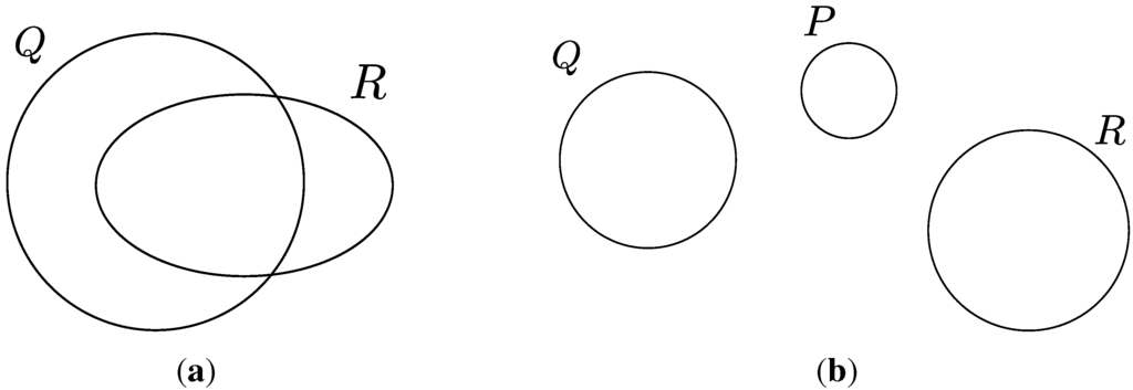
Figure 2. In (a) the object is nearly completely contained inside the object ; In (b) the object is between the objects and .

2.3. Map Generalisation

The International Cartographic Association defined generalisation as “The selection and simplified representation of detail appropriate to the scale and/or purpose of the map” [41]. Generalisation serves a variety of purposes including the creation and maintenance of spatial data at multiple scales, cartographic visualization at variable scales, and data reduction [42]. There exist many conceptual models, or frameworks, of the generalization process in both the manual and digital domains. An in-depth overview of these can be found in [41,43].

The goal of map generalization is to produce a suitable map representation subject to a set of constraints [44]. Weibel [45] identified Gestalt, semantic, metric and topological as four such constraints. A Gestalt constraint maintains important object shape characteristics. For example many authors have proposed aggregation techniques for buildings which maintain the shape characteristics of rectangularity [46,47] and symmetry [20]. Semantic constraints ensure generalization is performed in a manner which is a function of object semantics. Kieler et al. [48] and Haunert and Wolff [49] propose aggregation techniques which ensure that objects merged predominantly belong to the same class. Metric constraints perform generalization in a manner which is a function of an error function. Finally, a topological constraint attempts to ensure that the generalization process preserves topological relations between objects [44,50].

Map generalization is performed through the application of one or a number of generalization operators. Jones [51] identified eight categories of generalization operators. These are elimination, simplification, typification, exaggeration, enhancement, collapse, aggregation and displacement [50]. In this article we only consider the aggregation operator but a detailed discussion of operators which can be applied to buildings is contained in [52]. Aggregation may be defined as the replacement of a set of objects by a single object [53]. Replacing a set of house objects by a single housing estate object, as described in Section 1, is an example of aggregation. Regnauld [53] proposes that aggregation may be performed using one of the following four strategies. Aggregation with displacement displaces the set of objects until they touch or overlap and then subsequently merges these objects [54]. If the objects in question initially touch no displacement is necessary and they can be simply merged [48,49]. Aggregation by flooding replaces the set of objects in question with a single object of greater spatial extent such as the convex hull. Aggregation by sampling replaces the set of objects with a sub-set; this is also known as typification. Finally aggregation by connecting objects [3,46,55] is by far the most commonly used methodology and is the focus of the research presented here. We now describe in detail how this methodology functions.

Aggregation by connecting objects is generally performed in two steps. The first step of object grouping identifies sets of objects which require merging. The second step of object merging defines a set of connectors which connect the objects in each set; all objects and connectors in each set are then merged. For example consider the scene in Figure 3(a) containing the polygons and . In order to merge these objects we define one possible connector to be the polygon which is represented by the grey region in Figure 3(b). The merger of the two polygons is then defined as the union of the polygons and the corresponding connector; the result of which is represented by the polygon in Figure 3(c).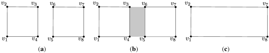

Figure 3. The two polygons in (a) are merged using the connected in (b) to give the result in (c).

Many authors have proposed methodologies which perform both steps of object grouping and merging [13,54,55,56]. Meanwhile some authors propose methodologies which perform a single step. For example Steinhauer et al. [14] and Qi and Li [15] describe techniques for object grouping alone. Methodologies which focus on the task of merging have mainly followed two approaches [53]. The first uses morphological operators (erosion and dilation) and are particularly suited to raster data [57]. The other trend uses the Delaunay triangulation geometrical structure and is suitable for vector data [13,54,55,56]. It should be noted that the aggregation of objects has many applications outside the domain of map generalization such as the generation of a shape, or footprint, from a set of points [58].

3. Proposed Model

As discussed in the introduction existing models of spatial relations do not consider that different concepts exist on different levels in a hierarchy and in turn that the spatial relations in a given scene are a function of the specific concepts considered. We propose that there exists two possible approaches to modeling a particular spatial relation. The first is to model the necessary higher level concepts explicitly using map generalization before inferring the existence of the spatial relation in question. The second approach is to model the necessary higher level concepts implicitly using a set of lower level concepts before inferring the existence of the spatial relation in question. For example, a housing estate may be modeled implicitly by set containing all houses belonging to the estate in question.

In this section we explore the former of these approaches by presenting a model of the spatial relation enters which may exist between a road and a housing estate. The model contains two steps. The first step performs object merging with the goal of creating an object corresponding to a housing estate. This facilitates inference with respect to the spatial relation in question. The second step performs this inference.

3.1. Generalisation Step

The proposed generalisation method performs only the task of object merging and assumes the set of objects which require merging is known a priori. An aggregation by connecting objects approach to merging is used which reduces the task of merging to one of defining a suitable set of connectors between the objects in question. An operator based on the Adapt Merge Operator of Ware et al. [54] is used to define the connectors in question. This choice of operator was motivated by the fact that Ware et al. [54] demonstrated that the Adapt Merge Operator achieves good results when applied to sets of polygons representing buildings. This operator functions as follows.

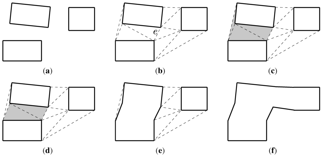
Figure 4. The three polygon in (a) are merged, through steps (b) to (e), to give the result in (f).

Given a set of polygons a constrained Delaunay triangulation is computed and all edges internal to polygons are removed. For example a scene containing three polygons and its corresponding triangulation are displayed in Figure 4(a,b) respectively. Next the shortest edge, denoted , in this triangulation which connects two different polygons is determined; these polygons correspond to the spatially closest in the scene. In Figure 4(b) the edge is labeled. The two polygons adjacent to and the corresponding set of connecting triangles are determined. This set of triangle is entitled . The set corresponding to Figure 4(b) contains three triangles and is represented by the grey region in Figure 4(c). Next a subset of , entitled , is obtained by removing those triangles which are not adjacent to and contain an edge of length greater than times the length of . corresponding to in Figure 4(c) contains two polygons and is represented by the grey region in Figure 4(d). and the two polygons adjacent to are then merged to form a single polygon. The result of applying this step to Figure 4(d) is displayed in Figure 4(e). This process of identifying and merging two polygons is then iterated until a single polygon remains. The result of merging the three polygons in Figure 4(a) is displayed in Figure 4(f).

The above merging operator does not prevent the introduction of intersections between the result of merging and other objects in the scene. For example consider the scene in Figure 5(a) which contains three polygons and a single line. The result of merging the three polygons using this method is displayed in Figure 5(b) where an intersection between the merged polygons and line exists.

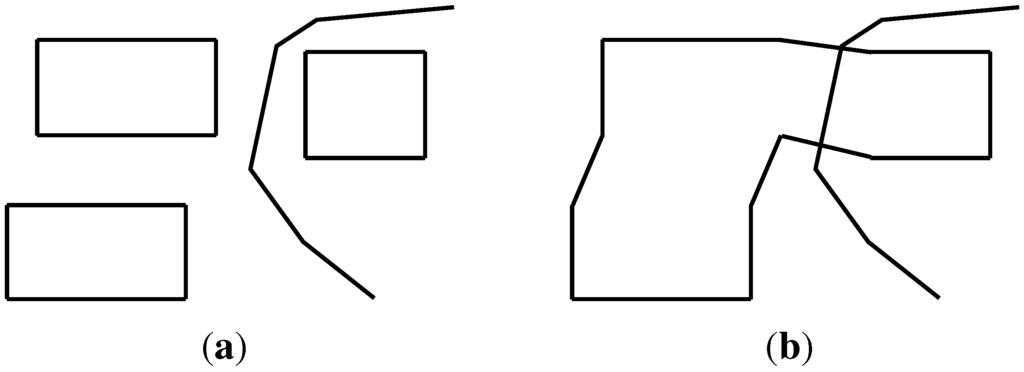
Figure 5. The merging of the polygons in (a) introduces a geometrical intersection with the line as illustrated in (b).

3.2. Inference Step

In this section we describe the function which determines the degree to which a line , corresponding to a road, enters a polygon , corresponding to a housing estate. is leveraged by another function which determines the degree to which a point , which lies on , enters . is a product of the functions and which measure the degree to which is surrounded by and close to the centroid of respectively. Having studied the spatial relation of enters in depth the authors believe both these attributes play a dominant role in its perception.

In order to compute we first generate a set of rays where is a ray with source and direction . For example in Figure 6 the set of rays for each corresponding point where are illustrated. Let be a function which returns a value of if intersects and returns a value of otherwise. is computed using Equation (1).

(1)

takes values in the interval . If lies inside , and is completely surrounded by , will evaluate to ; this is the case for the points in Figure 6(a,c). If does not lie inside , will evaluate to a number less than or equal to indicating the degree to which is surrounded by . This is the case for the point in Figure 6(b) where evaluates to . In our implementation a value of 720 was assigned to the variable which was found to provide a fine enough resolution.

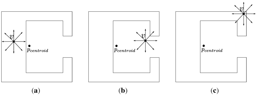
Figure 6. In each figure the set of 8 rays corresponding to a point are represented by arrows. represents the centroid of each polygon.

In order to compute we first compute the centroid, denoted , of . Next we compute the maximum distance, denoted , between and a point lying on the boundary of . This is computed using Equation (2) where is the set of vertices representing .

(2)

Let be the distance between and ; that is, . is computed using Equation (3).

(3)

takes values in the interval . Specifically, if is equal to , will evaluate to . If the distance between and is less than , will evaluate to a number in the interval decreasing with distance from . Otherwise will evaluate to . For example, corresponding to the scene in Figure 6(c) evaluates to a number close to because its distance from is close to . Meanwhile, due to the closer proximity of each to the centroid of , corresponding to the scenes in Figure 6(a) and (b) evaluates to and respectively. Having computed and we finally compute using Equation (4).

(4)

takes values in the interval . approaches the value as both function and approach the value . For example, the values corresponding to the scenes in Figure 6(a–c) are 0.71 ( ), 0.40 ( ) and 0.09 ( ) respectively. We now turn our attention to computing the degree to which a line enters a polygon , that is . Let specify that the point lies on the line . is defined by Equation (5).

(5)

Computing exactly represents a complex optimization problem for which we do not have a closed form solution. To overcome this difficulty we approximate this function using the following approach. We first select a set of points lying on where the distance between two consecutive points and , measured in terms of distance along the line, is constant. In our implementation we assigned equal to the length of measured in meters to give a distance of one meter between consecutive points.

4. Evaluation

In this section we evaluate the model of the spatial relation enters which was presented in Section 3. The remainder of this section is divided into three parts. Section 4.1 describes the data used in the evaluation. Section 4.2 presents a qualitative evaluation of the model. Section 4.3 demonstrates the model may be used to accurately classify housing estate access roads.

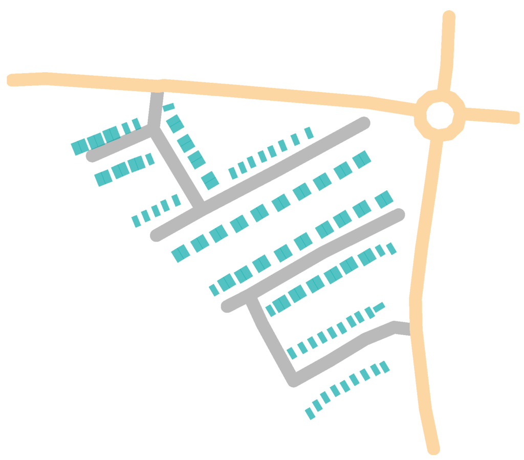
Figure 7. A set of polygons corresponding to houses in a housing estate and a number of lines corresponding to roads are represented. The grey lines represent the access roads for the housing estate in question. Data taken from OpenStreetMap.

4.1. Spatial Data

The data used in this study was taken from OpenStreetMap (OSM) (http://www.openstreetmap.org/). OSM is a form of volunteered geographic information (VGI) [59] which may be defined as the widespread engagement of large numbers of private citizens in the creation of geographical or spatial data. The following set of study areas, each of which is located in Ireland, were selected: Dublin city, Gorey County Wexford, Wexford town, Robertstown Kildare, Kilmeage Kildare, Carlow town. These specific areas were chosen because each is an urban area for which the corresponding OSM representation contains housing estates. A set of sixty scenes containing housing estates were selected. An effort was made to select a set of scenes which contained varied spatial patterns of houses. For each housing estate we identified a corresponding set of access roads and a corresponding set of roads in close proximity to the housing estate. Housing estates and corresponding roads were identified in each scene by visiting the location in question or, if this was not possible, using OSM semantic information and examining the location in question using Google Street View. According to the OSM wiki the correct tag for an access road is highway = residential. Many authors have proposed methods for grouping buildings which could potentially be used to automatically detect housing estates in OSM [12]. Figure 7 displays an example scene contained in our data set. The dataset was randomly divided into twenty scenes which were used for training and forty scenes which were used for testing our model. The result of applying the object merging methodology described in Section 3.1 to the test scenes in Figure 8(a,b) are displayed in Figure 8(c,d) respectively.

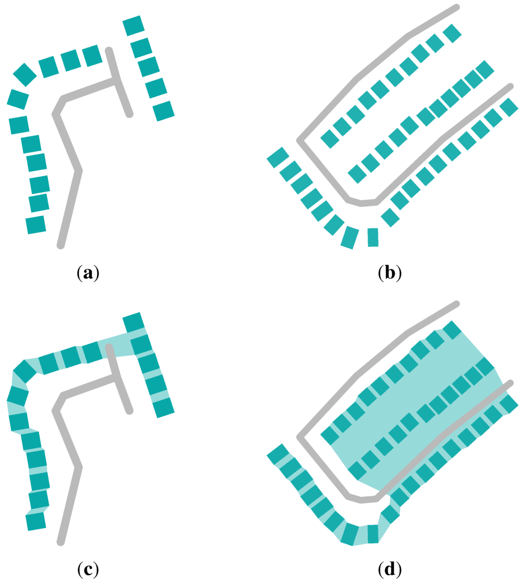
Figure 8. The results of merging the polygons in (a) and (b) are displayed in (c) and (d) respectively.

4.2. Qualitative Evaluation

Figure 9 displays a subset of the OSM test scenes with the corresponding value listed under each sub-figure. This particular subset was chosen to demonstrate the behavior of the model. It is evident from this figure that, in all those scenes where there is a strong perception that the road enters the housing estate, a high value ( ) is assigned. Specifically these are the scenes Figure 9(a,c,e,f,i,k). On the other hand it is evident that all those scenes where there is a strong perception that the road does not enter the housing estate a low value ( ) is assigned. Specifically these are the scenes Figure 9(b,d,g).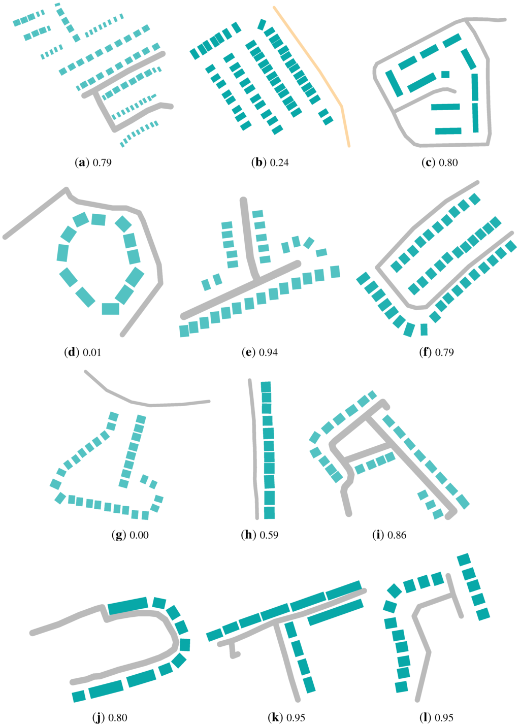

Figure 9. OSM test scenes with the corresponding values.

Examining Figure 9(h,j,l) we see that the relationship which exists between the housing estate and road could be described as both collinear and enters. Despite this fact the proposed model assigned a significantly high value of to each of these scenes. We argue that a scene may exhibit more than a single spatial relation.

Like all qualitative relations, enters may be present with varying degrees. It is unclear whether the proposed model of enters accurately captures the degree to which this spatial relation is present. For example consider the scenes in Figure 9(f,l) which have values of and respectively. Despite a significantly higher value of being assigned to Figure 9(l) relative to Figure 9(f), it is not evident that the relation of enters exists to a greater degree in Figure 9(l). This argument could also be applied to Figure 9(b,d). Determining how accurately the proposed model captures the degree to which the relation enters is present in a given scene would require a large scale behavioral study involving human subjects. As such, it is beyond the scope of this paper.

4.3. Access Road Classification

To demonstrate the usefulness of the proposed model we computed the accuracy with which it could classify the roads in the test scenes as access or non-access roads. Classification was performed using a threshold of which was determined using the training set. That is, a road was classified as an access road if the corresponding value was greater than ; otherwise it was classified as a non-access road. On the test set classification accuracy was achieved. To demonstrate that divides access and non-access roads into statistical significant groups an unbalanced analysis of variance (ANOVA) was performed [60]. It was found that the groups are statistical significant with .

5. Conclusions

This work represents the first attempt to model spatial relations in the presence of concepts which exist on different levels in a hierarchy. As such we believe it points the direction for future research in this area. Some possible future research directions include the following. Firstly it would be beneficial to consider other spatial relations, besides enters, which are a function of concepts which exist on different levels. As discussed in Section 4.2 modeling the spatial relation of collinear would be useful. The fusion of multiple relations may also require the application of techniques for recognizing spatial patterns so that the correct relation may be applied in a given case [61]. For future work it would be interesting to examine how other generalization operators, besides object merging, can play a role in modeling spatial relations. It would also be interesting to consider spatial relations between other spatial objects besides houses and roads. For example railway stations and railway lines.

In this work we proposed to model higher level concepts by explicitly computing the concepts in question using map generalization. However, as discussed in Section 3, higher level concepts may also be modeled implicitly as a set of lower level concepts. For example, a housing estate may be modeled implicitly by a set containing the corresponding set of houses without explicitly computing their merger. In future work we hope to explore the use of such implicit modeling of higher level concepts. It may be possible that some higher level concepts are more effectively modeled explicitly while others are more effectively modeled implicitly.

References

- Murphy, G. The Big Book of Concepts; MIT Press: Boston, MA, USA, 2002. [Google Scholar]
- Walter, V.; Luo, F. Automatic interpretation of digital maps. ISPRS J. Photogramm. 2011, 66, 519–528. [Google Scholar] [CrossRef]
- Tryfona, N.; Egenhofer, M.J. Consistency among parts and aggregates: A computational model. Trans. GIS 1997, 1, 1–3. [Google Scholar]
- Price, R.; Tryfona, N.; Jensen, C.S. Modeling Topological Constraints in Spatial Part-Whole Relationships. In Proceedings of the 20th International Conference on Conceptual Modeling: Conceptual Modeling, Yokohama, Japan, 27–30 November 2001; pp. 27–40.
- Egenhofer, M.; Wilmsen, D. Changes in Topological Relations when Splitting and Merging Regions. In Proceedings of the 12th International Symposium on Spatial Data Handling, Vienna, Austria, 12–14 July 2006.
- Mackaness, W.; Edwards, G. The Importance of Modelling Pattern and Structure in Automated Map Generalization. In Proceedings of Joint Workshop on Multi-Scale Representations of Spatial Data, Ottawa, ON, Canada, 7–8 July 2002.
- Touya, G. A road network selection process based on data enrichment and structure detection. Trans. GIS 2010, 14, 595–614. [Google Scholar] [CrossRef]
- Werder, S.; Kieler, B.; Sester, M. Semi-Automatic Interpretation of Buildings and Settlement Areas in User-Generated Spatial Data. In Proceedings of the 18th SIGSPATIAL International Conference on Advances in Geographic Information Systems, San Jose, CA, USA, 2–5 November 2010; pp. 330–339.
- Butenuth, M.; Gösseln, G.; Tiedge, M.; Heipke, C.; Lipeck, U.; Sester, M. Integration of heterogeneous geospatial data in a federated database. ISPRS J. Photogramm. 2007, 62, 328–346. [Google Scholar] [CrossRef]
- Anders, K.; Fritsch, D. Automatics interpretation of digital maps for data revision. Int. Arch. Photogramm. Remote Sens. 1996, 31, 90–94. [Google Scholar]
- Lüscher, P.; Weibel, R.; Mackaness, W. Where is the Terraced House? On the Use of Ontologies for Recognition of Urban Concepts in Cartographic Databases. In Headway in Spatial Data Handling; Ruas, A., Gold, C., Eds.; Springer: Berlin, Germany, 2008; pp. 449–466. [Google Scholar]
- Regnault, N. Recognition of Building Clusters for Generalization. In Proceedings of the 7th International Symposium on Spatial Data Handling, Delft, The Netherlands, 12–16 August 1996; pp. 185–198.
- Yan, H.; Weibel, R.; Yang, B. A multi-parameter approach to automated building grouping and generalization. Geoinformatica 2008, 12, 73–89. [Google Scholar]
- Steinhauer, J.H.; Wiese, T.; Freksa, C.; Barkowsky, T. Recognition of Abstract Regions in Cartographic Maps. In Proceedings of the International Conference on Spatial Information Theory: Foundations of Geographic Information Science, Morro Bay, CA, USA, 19–23 September 2001; pp. 306–321.
- Qi, H.B.; Li, Z.L. An approach to building grouping based on hierarchical constraints. Int. Arch. Photogramm. Remote Sens. Spatial Inf. Sci. 2008, XXXVII, 449–454. [Google Scholar]
- Zhang, X.; Ai, T.; Stoter, J. Characterization and Detection of Building Patterns in Cartographic Data: Two Algorithms. In Advances in Spatial Data Handling and GIS; Shi, W., Yeh, A., Leung, Y., Zhou, C., Eds.; Springer: Berlin, Germany, 2012; pp. 93–107. [Google Scholar]
- Christophe, S.; Ruas, A. Detecting Building Alignments for Generalisation Purposes. In Advances in Spatial Data Handling; Richardson, D., van Oosterom, P., Eds.; Springer: Berlin, Germany, 2002; pp. 419–432. [Google Scholar]
- Mao, B.; Harrie, L.; Ban, Y. Detection and typification of linear structures for dynamic visualization of 3D city models. Comput. Environ. Urban Syst. 2012, 36, 233–244. [Google Scholar] [CrossRef]
- Luscher, P.; Weibel, R.; Burghardt, D. Integrating ontological modelling and Bayesian inference for pattern classification in topographic vector data. Comput. Environ. Urban Syst. 2009, 33, 363–374. [Google Scholar] [CrossRef]
- Haunert, J. Detecting Symmetries in Building Footprints by String Matching. In Advancing Geoinformation Science for a Changing World; Geertman, S., Reinhardt, W., Toppen, F., Eds.; Springer: Berlin, Germany, 2011; pp. 319–336. [Google Scholar]
- Egenhoger, M.J.; Franzosa, R.D. Point-set topological spatial relations. Int. J. Geogr. Inf. Syst. 1991, 5, 161–174. [Google Scholar] [CrossRef]
- Shariff, A.; Egenhofer, M.; Mark, D. Natural-language spatial relations between linear and areal objects: The topology and metric of english-language terms. Int. J. Geogr. Inf. Sci. 1998, 12, 215–246. [Google Scholar]
- Hernandez, D. Qualitative Representation of Spatial Knowledge; Springer: Berlin, Germany, 1994. [Google Scholar]
- Cohn, A.G.; Hazarika, S.M. Qualitative spatial representation and reasoning: An overview. Fundam. Inform. 2001, 46, 1–29. [Google Scholar]
- Riedemann, C. Matching Names and Definitions of Topological Operators. In Spatial Information Theory; Cohn, A., Mark, D., Eds.; Springer: Berlin, Germany, 2005; Volume 3693, pp. 165–181. [Google Scholar]
- Cai, G.; Wang, H.; MacEachren, A.; Fuhrmann, S. Natural conversational interfaces to geospatial databases. Trans. GIS 2005, 9, 199–221. [Google Scholar] [CrossRef]
- Sjoo, K.; Jensfelt, P. Functional Topological Relations for Qualitative Spatial Representation. In Proceedings of the International Conference on Advanced Robotics, Montevideo, Uruguay, 20–23 June 2011.
- Egenhofer, M. Reasoning about Binary Topological Relations. In Proceedings of the Second International Symposium on Advances in Spatial Databases, Zurich, Switzerland, 28–30 August 1991; pp. 143–160.
- Egenhofer, M. A Reference System for Topological Relations between Compound Spatial Objects. In Advances in Conceptual Modeling—Challenging Perspectives; Heuser, C., Pernul, G., Eds.; Springer: Berlin, Germany, 2009; Volume 5833, pp. 307–316. [Google Scholar]
- Randell, D.; Cui, Z.; Cohn, A. A Spatial Logic based on Regions and Connection. In Proceedings of the International Conference on Knowledge Representation and Reasoning, Cambridge, MA, USA, 16–29 October 1992; 92, pp. 165–176.
- Knauff, M.; Rauh, R.; Renz, J. A Cognitive Assessment of Topological Spatial Relations: Results from an Empirical Investigation. In Spatial Information Theory A Theoretical Basis for GIS; Hirtle, S., Frank, A., Eds.; Springer: Berlin, Germany, 1997; Volume 1329, pp. 193–206. [Google Scholar]
- Renz, J.; Rauh, R.; Knauff, M. Towards Cognitive Adequacy of Topological Spatial Relations. In Spatial Cognition II, Integrating Abstract Theories, Empirical Studies, Formal Methods, and Practical Applications; Springer-Verlag: London, UK, 2000; pp. 184–197. [Google Scholar]
- Klippel, A. Spatial information theory meets spatial thinking—Is topology the Rosetta Stone of spatial cognition? Ann. Assoc. Am. Geogr. 2012. [Google Scholar] [CrossRef]
- Mark, D.; Egenhofer, M. Modeling spatial relations between lines and regions: Combining formal mathematical models and human subjects testing. Cartogr. Geogr. Inf. Syst. 1994, 21, 195–212. [Google Scholar]
- Egenhofer, M.; Mark, D. Naive Geography. In Spatial Information Theory A Theoretical Basis for GIS; Frank, A., Kuhn, W., Eds.; Springer: Berlin, Germany, 1995; Volume 988, pp. 1–15. [Google Scholar]
- Clementini, E.; di Felice, P.; van Oosterom, P. A Small Set of Formal Topological Relationships Suitable for End-User Interaction. In Advances in Spatial Databases; Abel, D., Chin Ooi, B., Eds.; Springer: Berlin, Germany, 1993; Volume 692, pp. 277–295. [Google Scholar]
- Cai, G.; Wang, H.; MacEachren, A. Communicating Vague Spatial Concepts in Human-GIS Interactions: A Collaborative Dialogue Approach. In Spatial Information Theory. Foundations of Geographic Information Science; Kuhn, W., Worboys, M., Timpf, S., Eds.; Springer: Berlin, Germany, 2003. [Google Scholar]
- Zhan, F.B. A Fuzzy Set Model of Approximate Linguistic Terms in Descriptions of Binary Topological Relations between Simple Regions. In Applying Soft Computing in Defining Spatial Relations; Matsakis, P., Sztandera, L.M., Eds.; Physica-Verlag GmbH: Heidelberg, Germany, 2002; pp. 179–202. [Google Scholar]
- Bloch, I.; Colliot, O.; Cesar, R.M., Jr. On the ternary spatial relation “between”. IEEE Trans. Syst. Man Cybern. B Cybern. 2006, 36, 312–327. [Google Scholar] [CrossRef]
- Raubal, M. Cognitive engineering for geographic information science. Geogr. Compass 2009, 3, 1087–1104. [Google Scholar] [CrossRef]
- Sarjakoski, L. Chapter 2 Conceptual Models of Generalisation and Multiple Representation. In Generalisation of Geographic Information; Mackaness, W., Ruas, A., Sarjakoski, L., Eds.; Elsevier Science B.V.: Amsterdam, The Netherlands, 2007; pp. 11–35. [Google Scholar]
- Weibel, R. Generalization of Spatial Data: Principles and Selected Algorithms. In Algorithmic Foundations of Geographic Information Systems; van Kreveld, M., Nievergelt, J., Roos, T., Widmayer, P., Eds.; Springer: Berlin, Germany, 1997; Volume 1340, pp. 99–152. [Google Scholar]
- Mackaness, W.A. Generalisation of Geographic Information: Cartographic Modelling and Applications; Mackaness, W.A., Ruas, A., Sarjakoski, L.T., Eds.; Elsevier Science B.V.: Amsterdam, The Netherlands, 2007. [Google Scholar]
- Jones, C.B.; Ware, J.M. Map generalization in the Web age. Int. J. Geogr. Inf. Sci. 2005, 19, 859–870. [Google Scholar] [CrossRef]
- Weibel, R. A Typology of Constraints to Line Simplification. In Proceedings of 7th International Symposium on Spatial Data Handling, Delft, The Netherlands, 12–16 August 1996; pp. 533–546.
- Regnauld, N.; Revell, P. Automatic amalgamation of buildings for producing ordnance survey 1:50,000 scale maps. Cartogr. J. 2007, 44, 239–250. [Google Scholar] [CrossRef]
- Haunert, J.; Wolff, A. Optimal and Topologically Safe Simplification of Building Footprints. In Proceedings of the 18th SIGSPATIAL International Conference on Advances in Geographic Information Systems, San Jose, CA, USA, 2–5 November 2010; pp. 192–201.
- Kieler, B.; Haunert, J.; Sester, M. Deriving scale-transition matrices from map samples for simulated annealing-based aggregation. Ann. GIS 2009, 15, 107–116. [Google Scholar] [CrossRef]
- Haunert, J.; Wolff, A. Area aggregation in map generalisation by mixed-integer programming. Int. J. Geogr. Inf. Sci. 2010, 24, 1871–1897. [Google Scholar] [CrossRef]
- Corcoran, P.; Mooney, P.; Winstanley, A.C. Planar and non-planar topologically consistent vector map simplification. Int. J. Geogr. Inf. Sci. 2011, 25, 1659–1680. [Google Scholar] [CrossRef]
- Jones, C.B. Geographical Information Systems and Computer Cartography; Prentice Hall: Upper Saddle River, NJ, USA, 1997. [Google Scholar]
- Regnauld, N.; McMaster, R. A Synoptic View of Generalisation Operators. In Generalisation of Geographic Information; Mackaness, W., Ruas, A., Sarjakoski, L., Eds.; Elsevier Science B.V.: Amsterdam, The Netherlands, 2007; pp. 37–66. [Google Scholar]
- Regnauld, N. Algorithms for the Amalgamation of Topographic Data. In Proceedings of the 21st International Cartographic Conference, Durban, South Africa, 10–16 August 2003.
- Ware, J.; Jones, C.; Bundy, G. A Triangulated Spatial Model for Cartographic Generalisation of Areal Objects. In Spatial Information Theory A Theoretical Basis for GIS; Frank, A., Kuhn, W., Eds.; Springer-Verlag: Berlin, Germany, 1995; Volume 988, pp. 173–192. [Google Scholar]
- Yang, L.; Zhang, L.; Ma, J.; Xie, J.; Liu, L. Interactive visualization of multi-resolution urban building models considering spatial cognition. Int. J. Geogr. Inf. Sci. 2011, 25, 5–24. [Google Scholar] [CrossRef]
- Li, Z.; Yan, H.; Ai, T.; Chen, J. Automated building generalization based on urban morphology and Gestalt theory. Int. J. Geogr. Inf. Sci. 2004, 18, 513–534. [Google Scholar] [CrossRef]
- Damen, J.; van Kreveld, M.; Spaan, B. High Quality Building Generalization by Extending the Morphological Operators. In Proceedings of the ICA Workshop on Generalization, Montpellier, France, 20–21 June 2008.
- Dupenois, M.; Galton, A. Assigning Footprints to Dot Sets: An Analytical Survey. In Spatial Information Theory; Hornsby, K., Claramunt, C., Denis, M., Ligozat, G., Eds.; Springer: Berlin, Germany, 2009; Volume 5756, pp. 227–244. [Google Scholar]
- Goodchild, M. Citizens as sensors: The world of volunteered geography. GeoJournal 2007, 69, 211–221. [Google Scholar] [CrossRef]
- DeGroot, M.; Schervish, M. Probability and Statistics, 4th ed; Pearson: London, UK, 2011. [Google Scholar]
- Zhang, X.; Ai, T.; Stoter, J.; Kraak, M.; Molenaar, M. Building pattern recognition in topographic data: Examples on collinear and curvilinear alignments. GeoInformatica 2013, in press. [Google Scholar]
© 2012 by the authors; licensee MDPI, Basel, Switzerland. This article is an open-access article distributed under the terms and conditions of the Creative Commons Attribution license (http://creativecommons.org/licenses/by/3.0/).