Article

Adjustable and Adaptive Control for an Unstable Mobile Robot Using Imitation Learning with Trajectory Optimization

Automatic Control, Technical University of Munich, 80333 Munich, Germany
*
Author to whom correspondence should be addressed.
Robotics 2020, 9(2), 29; https://doi.org/10.3390/robotics9020029
Submission received: 21 February 2020 / Revised: 16 April 2020 / Accepted: 22 April 2020 / Published: 25 April 2020

Abstract

:
In this contribution, we develop a feedback controller in the form of a parametric function for a mobile inverted pendulum. The control both stabilizes the system and drives it to target positions with target orientations. A design of the controller based only on a cost function is difficult for this task, which is why we choose to train the controller using imitation learning on optimized trajectories. In contrast to popular approaches like policy gradient methods, this approach allows us to shape the behavior of the system by including equality constraints. When transferring the parametric controller from simulation to the real mobile inverted pendulum, the control performance is degraded due to the reality gap. A robust control design can reduce the degradation. However, for the framework of imitation learning on optimized trajectories, methods that explicitly consider robustness do not yet exist to the knowledge of the authors. We tackle this research gap by presenting a method to design a robust controller in the form of a recurrent neural network, to improve the transferability of the trained controller to the real system. As a last step, we make the behavior of the parametric controller adjustable to allow for the fine tuning of the behavior of the real system. We design the controller for our system and show in the application that the recurrent neural network has increased performance compared to a static neural network without robustness considerations.

1. Introduction

The control of mobile and unstable systems is, in most cases, divided into a stabilizing and a maneuvering part, e.g., [1]. This breakdown of the problem into two separate tasks makes analytic control designs manageable, however, the final performance of the system will be limited compared to holistic approaches. General holistic approaches are difficult to derive analytically for nonlinear systems. Thus, methods based on optimization and learning come into play that train a control law in the form of a parametric function based on a cost function. Most notably, methods emerged from the field of reinforcement learning, e.g., policy gradient methods like PPO [2], are used, as well as methods from the field of gradient-free optimization. For systems with relatively slow dynamics, nonlinear model predictive control can be used [3], which is, however, not suited for fast systems due to the continuous online optimization with non-deterministic computing time. In this work, we design a parametric controller for the position and orientation control of a mobile inverted pendulum (MIP), without the need to compute trajectories online.
The control laws derived based on the aforementioned approaches are generally trained in a simulation environment and often do not transfer well to the real system due to model inaccuracies, also called the reality gap. In order to overcome this challenge, different approaches have been developed. Some methods update or learn a highly precise model online, in order to reduce the reality gap [4,5]. Other approaches use adversarial attacks during the training of the controller in order to enforce robustness [6,7]. Other works focused on training a controller that is trained on a multitude of varying model dynamics, also called model ensembles [8,9,10]. The current research on overcoming the reality for this type of control law is mostly focused on methods of the domain of reinforcement learning. In this work, we tackle the reality gap problem for a less common class of design methods.
We use a method that is related to imitation learning [11] and has been referred to as a form of explicit model predictive control [12]. The method was also mentioned in [13], where a more complex and expensive optimization problem was then derived. In a second step, we extend the method to adapt online to model uncertainties by using a dynamic control law in the form of a recurrent neural network and by randomizing model parameters during training. Different from Peng et al. [9] who also use a dynamic control law, our method is based on the imitation learning framework instead of reinforcement learning, which allows us to shape the behavior of the system using equality constraints. With the objective of the application on the real system, we also make the behavior of the final control law adjustable by an external user via a trivial extension of the method.

2. Related Work

This section gives an overview of methods and research in two different areas related to our approach. The first area deals with the learning of parametric controllers that have a similar control performance in simulation and in the application on a real system. The second area is concerned with learning parametric controllers, based on a combination of imitation learning and trajectory optimization.

2.1. Training Robust Parametric Controllers

Most parametric controllers are trained in simulation due to the high cost of real-world data. The gap between the simulation model and reality can lead to poor performance or even failure of the controller when applied to the real system. Many articles have been published that either tackle the problem of reducing the reality gap or train a controller that can perform well despite the reality gap.
In order to improve the accuracy of the simulation model and as such reduce the reality gap, data concerning interactions with the real system have to be considered. Abbeel et al. [14] use an iteratively updated model to compute an improvement direction for the control parameters using a policy-gradient method. The step-size of the update is, however, determined on the real system. This is beneficial, as determining a good step size requires less interaction with the real system than estimating a gradient direction. The model is retrained after each update of the control parameters with new data. In Deisenroth and Rasmussen [4] a model in the form of a Gaussian Process is iteratively updated and a control improvement is done offline after each update, using gradient descent on the accumulated costs. In Golemo et al. [5], the model error is approximated using a recurrent neural network, trained on data from the real system, and a controller is then derived in simulation using the policy-gradient algorithm PPO [2].
Recently, more and more works focus on designing controllers that are robust with regards to model errors, rather than further increase the model accuracy. The methods can be roughly classified in methods that use a multitude of model parameters for training and methods that use a disturbing entity, called the adversary. A set of different model parameters is used in Mordatch et al. [15] to compute robust trajectories for a humanoid robot. As such, this work does not fall completely in the scope of robust parametric control, but rather robust trajectory generation. A non-parametric controller was used to deal with small system deviations online. Rajeswaran et al. [8] propose to train robust controllers using randomizing model parameters and a policy-gradient algorithm, while using only a subset of the worst trajectories to approximate the policy-gradient. This can be seen as a relaxation of a min-max formulation, common in nonlinear robust control [16]. An adversarial approach is introduced in Pinto et al. [7] to train a robust controller. Both the controller and the adversary are parametric functions that are trained using a policy-gradient algorithm. The approach also approximates the min-max problem, with the robust controller minimizing the total costs, and the adversary maximizing them again through bounded adversary actions. A different approach is presented in Yu et al. [17]. Instead of approximating a min-max solution, the parametric controller is trained with uncertain model parameters as additional inputs using the policy-gradient algorithm TRPO [18]. As the parameters of the real system are unknown during the application, an estimator/observer is trained in a second step, and the union of both estimator and controller are able to adapt to the real dynamics by guessing the current system parameters during application. Pattanaik et al. [6] fool the policy during training by perturbing the perceived state. In this case, the perturbations, or adversary attacks, do not result from a second controller but are either sampled randomly or computed based on the action-value function. Muratore et al. [10,19] use randomized model parameters to estimate the simulation optimization bias and prevent the learned policy from overfitting to the simulator. While the focus of Bousmalis et al. [20] lies on their vision component, the model parameters of the simulated robot arm are also randomized in order to improve the robustness. Peng et al. [9] train a recurrent neural network using reinforcement learning, while randomizing the model parameters. While the recurrent neural network only sees the current states and needs to learn a hidden state representation, the critic, i.e., the action value function, is omniscient in the sense that it has the model parameters as additional input. Chebotar et al. [21] also randomize model parameters, but focus their contribution on adapting the distribution of the model parameters iteratively by also including interactions of the real system. The policy is again learned using the policy-gradient algorithm PPO [2].
When looking at existing literature in this field, it is noticeable that the parametric controllers are solely trained using policy-gradient algorithms. In the present time, the most widely used methods to train a parametric controller stem from the field of reinforcement learning. However, alternatives exist and every method has its own strengths and weaknesses. Some methods from the field of gradient-free optimization, most notably evolution strategies, have proven to be competitive or even superior in certain cases [22,23]. Reinforcement learning algorithms learn by exploring in action-space and by increasing the probability of better than average actions, while evolution strategies explore in parameter space and increase the probability of better than average parameters [24]. Yet another class of algorithms to learn parametric controllers, which is in the focus of our contribution, is a combination of trajectory optimization and supervised learning. This can be seen as a special case of imitation learning. This last class of algorithms proved to be the best suited for the task at hand for reasons mentioned later, but methods focusing on robustness and transferability have to date not been investigated upon to the best of our knowledge.

2.2. Imitation Learning with Trajectory Optimization

As the name imitation learning suggests, the field is concerned with learning a parametric control law that imitates the behavior of a teacher, based on demonstrations on how to solve the task. In most of the current literature concerned with imitation learning, the expert is considered to be a human. A survey on applied methods with a human expert can be found in [11]. Since we will not have a human expert, we only consider, with a few exceptions, related works where the teacher is not a human but an optimizer. The approach of training a controller by combining trajectory optimization with supervised learning is far from new, yet no umbrella name for these methods has been established in literature. In this paper, we refer to these methods as imitation learning with trajectory optimization. The following literature contains works from both the control and machine learning communities.
An early application of this method is found in [25], where a neural network is trained as a controller for a wheeled robot. The task is to follow a desired path while avoiding obstacles with results also shown in the real application. An implementation with results in simulation for a chemical process can be found in Åkesson et al. [26]. An application for the control of a semi-active suspension system of the same method is shown in [12] where the authors report improved control performance with regards to their previous analytic control design.
Ross et al. [27] tackle a fundamental problem of imitation learning: the states visited by the expert during the demonstration and later used for supervised learning and the states that the controller will visit during execution are not distributed equally. Therefore, they propose an iterative approach where the controller samples states during execution and the expert provides actions for those states, rather than showing his own solution to the task. The training data obtained in this way is aggregated in a growing data-set. The method, called DAGGER for data-set aggregation, was proposed for use with human experts. He et al. [28] use DAGGER with an artificial expert. In each iteration their expert generates actions that are suboptimal, yet close to the current controller, with the intention of creating actions that can be learned faster than the optimal action. They show small improvements with regards to an expert that always generates optimal actions. Laskey et al. [29] propose adding noise to an artificial expert’s demonstrations with the aim of learning a policy that is able to recover from errors. The power of the noise is optimized such that the distribution of expert trajectories approaches the distribution of trajectories produced by the parametric controller in the loop. The approach is called DART for “disturbances for augmenting robot trajectories”.
Mordatch and Todorov [13] combine the trajectory optimization step with the supervised learning step by combining their objectives into a single optimization problem: minimizing costs of states and actions (trajectory optimization) and learning a parametric controller that can reproduce similar actions (supervised learning step). They then solve the optimization problem by iterating between regularized trajectory optimization and supervised learning. On simulation tasks, they show a decrease in the expected costs for their method, compared to a separation of trajectory optimization and supervised learning. In a later work [30], Mordatch et al. show the performance for more complex simulations and add a small number of recurrent states as well as sampled noise to their optimization setting.
Levine and Koltun [31,32] formulate a similar idea as a stochastic optimization problem by minimizing the Kullback-Leibler divergence between the distribution of actions produced by the controller and the actions of a distribution with high probability of low costs. They name their approach guided policy search. Guided policy search is also used by Zhang et al. [33] for the obstacle avoidance of a simulated quadrotor. However, they use a simulation of a model predictive controller (MPC) instead of optimizing the trajectory as a whole, and the supervised learning step uses only a subset of the states that the MPC was allowed to use. They extend their algorithm for the simulated quadrotor problem in Kahn et al. [34] to use an adaptive MPC during data generation and call their approach PLATO. As such, the final controller works on states that are available during real flights instead of the augmented state representation available to the MPC. Guided policy search also allows Levine et al. [35] to learn a convolutional neural network controller for a physical robot arm, using only pixel data as control inputs.
We refrain from using the previously mentioned methods, coupling supervised learning and trajectory optimization into a single objective, due to the increase in computation time and complexity and our focus on transferability to the physical system.

3. Design of an Adaptive and Adjustable Controller Using Imitation Learning

In this section, we present a new approach for training a parametric controller offline that is robust to model uncertainties by adapting to the system’s behavior during execution. The approach uses randomized dynamics and a controller with internal states, e.g., a recurrent neural network. The idea has similarities to [9], however, we use imitation learning with trajectory optimization instead of reinforcement learning. Different from [9], the approach that is introduced in this section can use time-dependent cost functions and equality constraints to define the behavior of the system. The inclusion of equality constraints is essential for the control design of our system, as is explained later in Section 5.1. While the final controller has recurrent states to account for model uncertainties similar to [9], the training method and therefore the admissible problem setting differ fundamentally. Moreover, the presented approach consists of a sequence of well established and understood sub-problems, whereas the success of reinforcement learning algorithms depends on hyper-parameters that can be difficult to tune [36].
Training a controller using supervised learning on optimized trajectories does not work for controllers with recurrent states. We leverage the problem by using ideas similar to DAGGER [27] and DART [29]. The approach uses an intermediate policy with model parameters as input, similar to the universal policy in [17], which is necessary to reduce computation time to an acceptable level. The intermediate policy is called the oracle network and acts as a teacher for the final recurrent controller. The oracle network itself can only be used in simulation, whereas the recurrent controller is suitable for both simulation and application.
The approach is divided into three consecutive optimizations and does not require the real system in the loop. The three main parts are
  • Trajectory optimization with randomized model parameters.
  • Training an intermediate oracle network.
  • Training of a controller with internal states.
We also show a trivial extension of the approach, in order to make the final controller adjustable by the operator. In the case of, e.g., a neural network controller, the parameters of the controller are not interpretable as is the case, e.g., for PID controllers. By making the controller adjustable, we do not have to repeat the whole optimization if only a small change in the behavior is required.
In the following we assume a dynamics model that is discretized in time and continuous in the state and action space. We denote the system state at time t by x t R n and the control signal, or action u t R m . We also assume for simplicity that the dynamics model is deterministic, as is most often the case for models that are derived from laws of physics. The dynamics also depend on constant but possibly uncertain parameters p , e.g., friction coefficients, moments of inertia. The nonlinear state space model is of the form
x t + 1 = f ( x t , u t ; p ) .

3.1. Trajectory Optimization

The first part of our method consists of creating and storing optimal trajectories starting from relevant initial states. We also limit ourselves to trajectories over a fixed time horizon T. A distribution D x 0 ( x ) over relevant starting states x 0 is defined by the control engineer. If a policy is directly derived using supervised learning on the trajectories, it is necessary to include starting states in D x 0 ( x ) with velocities that are diverging from the desired state or trajectory. Otherwise, the learned policy will not be able to recover once diverging, e.g., because of a perturbation or simply because of modeling errors. In order to have a robust policy at the end, we also want to define a distribution over uncertain model parameters D p ( p ) . Moreover, the control engineer has to define the time horizon T over which the trajectories are optimized and provide a cost function c ( x t , u t ) and end costs c T ( x T ) defining the behavior and goal of the control.
Let X = [ x 0 , x 1 , , x T ] and U = [ u 0 , u 1 , , u T 1 ] be the states and control inputs of a trajectory. An optimal trajectory for a given starting state x 0 D x 0 ( x ) and parameter set p D p ( p ) is calculated by solving:
( X * , U * ) = arg min X , U t = 0 T 1 c ( x t , u t ) + c T ( x T )
s . t . x t + 1 = f ( x t , u t ; p )
x t = 0 = x 0
eq ( X , U ) = 0
ieq ( X , U ) 0 .
Equations (2d) and (2e) represent equality and inequality constraints, which can be used to consider e.g., bounded control inputs or to enforce convergence to a specific terminal state x T , ref . If the control signals are not smooth, the inequalities can also be used to enforce smooth signals. This is advised as the control will be approximated by a smooth function approximator later.
The problem in Equation (2a) can be solved by either indirect or direct methods [37]. We choose a direct method called multiple shooting [38], as the method works naturally with discretized dynamics and direct methods are known to converge better than indirect methods for initializations that are far from the optimal solution. On the other hand, direct methods are known to produce less accurate solutions. For direct multiple shooting, all equality constraints, i.e., Equations (2b) and (2d) are handled using Lagrange multipliers. Either sequential quadratic programming or interior point methods, also called barrier methods, can be used to solve the problem including inequality constraints [39]. We use an open-source solver IPOPT [40], which implements an interior point solver.
It is important to note that the optimal action u * for a state x can be ambiguous due to the finite optimization horizon T, as well as the constraints (2d)–(2e). The finite horizon and the optimization constraints can cause the optimal u * to not only depend on a state x but also on the time t, i.e., whether the state x was visited early or late in the trajectory. As an example, consider the problem
( X * , U * ) = arg min X , U t = 0 3 x 2
s . t . x t + 1 = x t + u t
x 0 = 1 ; x 3 = 1
where the constraint x 3 = 1 forces the trajectory to return to a region of high costs. The solution to the problem is X * = [ 1 , 0 , 0 , 1 ] and U * = [ 1 , 0 , 1 ] . In this artificial example, the state x = 0 is visited at t 1 , 2 , and the optimal actions are u 1 = 0 , u 2 = 1 .
Thus, in order to provide unambiguous training targets, only the first optimal state-action pair ( x 0 * , u 0 * ) would have to be used. That would however be computationally very expensive, which is why we will use all state-action pairs ( X * , U * ) during training. We believe that for any problems with non-neglectable optimization time, the trade-of of introducing ambiguous state-action targets by using all state-action pairs of the trajectories can be justified by the reduction in computation time.
The optimization in Equation (2) is performed multiple times for different x 0 D x 0 ( x ) , p D p ( p ) until a sufficient coverage of the distributions is achieved. The N optimal trajectories, together with the corresponding model parameters p are stored for later use as tuples ( X k * , U k * , p k ) ; k { 1 , , N } .

3.2. Oracle Training

After a multitude of optimal trajectories has been obtained, we train a controller that uses both the state x t and model parameters p as inputs, similar to Yu et al. [17]. This controller can only be used in simulation when the model parameters are known. However, it would be problematic to guess good parameters when applying the control to the real system. Therefore, this controller is only an intermediate result and will be used as a teacher for the recurrent controller.
The control law is represented by a parametric function u t = g ( x t , p ; Θ ) . Our intermediate controller is learned using supervised learning on state-action pairs of the optimal trajectories. This is a simple regression problem and optimal parameters can be found by solving a regression problem:
Θ * = arg min Θ κ k = 1 N t = 0 T 1 u t , k g ( x t , k , p k ; Θ ) 2
with κ = 1 N · ( T 1 ) .
In order to avoid overfitting onto the data, it is generally advised to use cross-validation, i.e., to split the data into a dataset for training and a dataset to test the model performance.
The best way to solve (4) depends on the parametrization of g ( ) . We use fully connected neural networks in this paper and solve Equation (4) using stochastic gradient descent with the optimizer Adam [41]. We call this intermediate parametric controller the oracle, as it is provided with the full model information to generate its output.

3.3. Training a Robust Recurrent Network

As previously mentioned, the control law obtained in Section 3.2 is not suited for use on a physical system, as it requires knowledge of the underlying parameters, which we assume uncertain. We circumvent this problem by learning a control law that adapts to the dynamics of the system. As in Peng et al. [9], the new control law will use the history of past states and actions to generate the new control signal:
u t = g ( x t , u t 1 , x t 1 , , u 0 , x 0 ; Θ ) .
as the state transitions and thus the history ( x t , u t 1 , x t 1 , , u 0 , x 0 ) are different for each parameter set p , a control law in the form of (5) can produce different control outputs for different p .
The parametrization of a function in the form of (5) would be inefficient, therefore a common approach is to learn a representation of the past history as an internal state h t , also called hidden state. A recurrent neural network is an example for such a representation. The general structure of recurrent neural networks is:
h t = r 1 ( x t , h t 1 ; Θ 1 )
u t = r 2 ( h t ; Θ 2 ) .
We mostly use a shorter notation with Θ = [ Θ 1 T , Θ 2 T ] T , combining (6a) and (6b) into a single function. The shorter notation for a recurrent network is then
[ u t T , h t T ] T = r ( x t , h t 1 ; Θ ) .
Unlike the system state x t , the learned hidden state is generally not interpretable as a physical quantity.
The training of the parameters Θ for recurrent neural networks using supervised learning is usually done using backpropagation through time. A loss between training inputs and training outputs is defined and a gradient is computed over a sequence of data. For regression problems, the mean squared error is used.
[ Θ 1 * , Θ 2 * ] = arg min Θ 1 , Θ 2 κ k = 1 N t = 0 T 1 u t , k r 2 ( h t , k ; Θ 2 ) 2
s . t . h t , k = r 1 ( x t , k , h t 1 , k ; Θ 1 )
h ( 1 ) , k = 0 .
Training recurrent neural networks is computationally more expensive, as the gradient is computed by backpropagating through a sequence, which is similar to backpropagating through a deep neural network with the depth growing according to the sequence length. For long sequences, it is common to accept a bias in the gradient direction by truncating long sequences into smaller chunks [42]. Computing the loss gradient over truncated sequences is called truncated backpropagation through time (TBPTT).
A naive training of a recurrent neural network on sequences generated during the trajectory optimization will not lead to a good control law in the closed loop. This is due to the fact that sequences in the training data and the sequences seen during execution of the controller stem from different distributions. All training sequences are sequences included in optimal trajectories. Once the controller deviates from those trajectories, no training data is available. To leverage the problem, we use a mixture of ideas from DAGGER [27] and DART [29] together with our artificial expert trained according to Section 3.2. We train our recurrent neural network on sequences seen during execution of the recurrent neural network, but with actions recommended by the oracle network. Our small changes to DAGGER are the fact that we do not accumulate datasets, but learn for a limited number of iterations on the last data-set only. This is motivated by the fact that data generation using our artificial expert is cheap and early trajectories will not be relevant for the sequences that the final controller will produce. Early trajectories can thus be discarded for reasons of efficiency. Similar to DART we also add a small noise to the data gathering to have more variance in the sequences, especially close to convergence. However, we add our noise to the learning controller instead of to the expert. That way the distribution of sampled trajectories is always close to trajectories of the learning controller and we do not have to minimize the Kullback-Leibler divergence between two distributions, as is done in DART. Pseudo-code for generating training data for the recurrent neural network is give in Algorithm 1. Pseudo-code of our DAGGER and DART combination, which we abbreviate in the following as disturbed oracle imitation (DOI), is shown in Algorithm 2.
A visual comparison of the three algorithms DAGGER, DART and DOI is given in Figure 1. DAGGER generates training data on the trajectory created by the controller in the loop and accumulates all data. DART generates data for a distribution of trajectories generated by an expert, with the distribution variance adapted to the trajectories of the controller. DOI generates data on trajectories close to trajectories of the controller in the loop, but does not accumulate past data.
Algorithm 1 Generating training data for the recurrent neural network
Inputs: g , D x 0 , D p 0 , ϵ
x 0 D x 0 ( x ) , p D p 0 ( p ) , h ( 1 ) = 0
for t = 0 to T do
      u ^ t = g ( x t , p )
      u t , h t = r ( x t , h t 1 ; Θ )
      x t + 1 = f ( x t , u t ; p ) + N ( 0 , ϵ 2 I )
end for
return X = [ x 0 , , x t 1 ] , U ^ = [ u ^ 0 , , u ^ t 1 ]

▹ Evaluate oracle
▹ Evaluate controller
▹ Disturbed dynamics
Algorithm 2 Disturbed Oracle Imitation (DOI)
for epoch = 1 to N e p o c h do
      D
     for traj = 1 to N t r a j do
          sample sequence X traj , U ^ traj
           D D X traj , U ^ traj
     end for
     for gd = 1 to N g d do
          Update Θ using TBPTT.
     end for
end for
At this point, the reason for the oracle network has to be clarified, since it is a reasonable assumption that one could just solve the optimization problem in Equation (2) to generate the training targets u ^ t for each x t in Algorithm 1. The reason is again the computational burden, as only the first action of the optimized trajectory would be used. Solving this many trajectory optimizations would only be feasible for small problems. Also, problems occur when a state is visited by the recurrent controller in early iterations where the trajectory optimization is unfeasible due to constraints. By creating the intermediate network, all T 1 actions in the optimized trajectories can be used.
For the problem in this paper presented in Section 4, the trajectory optimization is the most expensive part and T = 500 . A direct use of the optimizer to create training targets u ^ t had to be interrupted due to the extremely slow progress.

3.4. Adding Adjustable Behavior

The training of parametric controllers can require a lot of computation time. If the controller does not perform in the desired manner on the real system, the lengthy procedure needs to be repeated and time is lost. By a trivial extension of the presented method, we show how we can make the behavior of the controller adjustable. In the case of simple controllers, e.g., PID controllers, it is common practice to tune the final behavior in the closed loop with the real system [43]. For parametric controllers, however, simply tuning the parameters is not appropriate, as the influence of the change cannot be predicted and the number of parameters is usually high.
The behavior of the controller in our approach is defined by the cost function in Equation (2a). In a similar fashion as we design a controller to work on multiple models, we can design a controller to work on multiple cost functions.
In an initial step, the cost function is augmented to depend on an additional parameter λ in a bounded range, e.g., λ [ 1 , 1 ] . The influence of the parameter can be, e.g., to shift between penalizing large control signals and penalizing the state costs. The optimal trajectories are then initialized with random initial states and model parameters as well as a cost function parameter sampled from a uniform distribution covering the range. This can also be interpreted as augmenting the state x t with an additional state λ , with dynamics λ t + 1 = λ .
The oracle network g λ ( x t , p , λ ; Θ ) is then trained using supervised learning on the optimal trajectories. The recurrent controller has the state x and λ as inputs:
[ u t T , h t T ] T = r λ ( x t , λ , h t 1 ; Θ ) .
The parameter λ is constant during execution and set by the control engineer. It can be used to adjust the behavior without training a new controller.

4. Task and Model Description

In this section, the mobile inverted pendulum is shortly presented and the control task is clarified. The mathematical model that is used to create the controller is also provided.

4.1. System and Task

The mobile inverted pendulum (MIP) is an unstable system with a non-holonomic contraint, described by a nonlinear model. A schematic and a picture of the hardware are shown in Figure 2. The wheels are accelerated by two DC motors. The sensors include a gyroscope, an accelerometer and encoders attached to the motors. The actuation signal for the motors and the sensor signals are handled by a microcontroller, which also communicates with a Raspberry Pi. The Raspberry Pi is used to evaluate the control law, as memory and computing power of the microcontroller are insufficient for the evaluation of our neural network.
Because of the challenging system properties of the MIP, it has been extensively studied in the control community. Control laws for the mobile inverted pendulum are often designed around a linearized model and the system is only operated within small tilt angles and target positions in close proximity of the MIP. Controllers based on linearized models can be found, e.g., in [44,45]. An example of a control design based on a nonlinear model is given in Ha et al. [46], however results are only given in simulation.
The task considered in this work is to design a controller for the MIP allowing it to autonomously drive to a desired position, not necessarily in close proximity, and take a desired orientation. The controller furthermore has to stabilize the tilt angle while driving and it has to be computationally cheap enough to be evaluated in real time ( δ t = 0.01 s ) on the Raspberry Pi.
Let x and y be the position coordinates in an inertial coordinate system I and γ the yaw angle of the MIP. While we want to drive to any position x r , y r and orientation γ r in the inertial coordinate system later, it is sufficient to learn a controller that can drive to a single point and orientation e.g., [ x r , y r , γ r ] = 0 . A coordinate transform in Equation (10) allows us to place any reference point different from 0 in the inertial coordinate system I into the origin of a second coordinate system B, and we can then use x B , y B and γ B for control.
[ δ x , δ y ] T = [ x x r , y y r ] T
x B y B = cos ( γ r ) sin ( γ r ) sin ( γ r ) cos ( γ r ) δ x δ y
γ B = γ γ r .

4.2. Mathematical Model

The mathematical model of the MIP consists of the body dynamics and the electric drive model. We adopt the model presented in Pathak et al. [47] for our rigid body dynamics. The model has seven states: x = [ x , y , γ , α , α ˙ , v , γ ˙ ] T . The state variables consist of the position in the inertial coordinates x , y , the yaw angle γ and its time derivative γ ˙ , the tilt angle α with time derivative α ˙ and the forward velocity v. The equations of the body dynamics model are derived in [47] are repeated in the Appendix A.
The electric drive model consists of a standard model for DC motors found, e.g., in [48], with parameters determined through identification using measurement data. We neglect the current dynamics in our motor model, as they are much faster than the rest of the system’s dynamics. We also add a heuristic friction model with four parameters c fric , 1 - 4 . We combine the motor torque constant k 2 with the resistance, to reduce the number of parameters to identify, since we are only interested in the input-output relationship and not real physical values. Our friction and drive model are given in Equation (11).
τ fric = c fric , 1 · tanh ( c fric , 2 · ω ) · e c fric , 3 · ω 2 + c fric , 4 · ω
τ = k 2 · ( u k 1 · ω ) τ fric
The identified and measured parameters for drive, friction and body dynamics are given in Table 1. The parameters c z , I y y and c fric , 1 are assumed uncertain for the control design and are depicted as a range, since they are hard to determine with high precision and the model dynamics are sensitive to changes in their value.

5. Application and Results

In this section, we first provide the settings and details of the approach presented in Section 3 for our application on the MIP. Then, a short analysis of training properties and results on the robustness are given both in simulation and on the real system. Our final recurrent controller of the form in Equation (9) is compared with different static controllers and the oracle controllers in terms of different robustness metrics. The oracle controllers are given only as a reference in the simulation results as a baseline for the performance of the recurrent controllers, however, as mentioned earlier, the oracle controllers cannot be used in the real application.

5.1. Control Design Details

The first part of our approach consists of the trajectory optimization. We optimize N = 10,000 trajectories for each controller. We show, however, that the task can be solved using less trajectories. The large number of trajectories reduces the influence of random sampling for our results. We sample three data sets. The first data-set, which is used to train a reference controller, has varying initial states with constant model parameters and a constant cost function. The second data-set has varying initial states and model parameters, with a constant cost function. The third data-set includes varying initial states, model parameters and the cost function parameter.
The initial states are sampled from uniform distributions. All entries of the initial state vector x are perturbed, which is important to include starting states of a falling MIP and thus to receive trajectories of the MIP recovering from falling. The initial positions are sampled in a radius of 1.1 m around the origin of the inertial coordinate system. The maximum range we consider for the control later is 1 m; all target points outside of this range are projected back onto the radius.
The optimization horizon is 501 steps from t = 0 to t = T = 500 , with a discrete step size of δ t = 0.01 s . Each trajectory is thus 5 s long. For the first two data-sets, we minimize the accumulated costs in Equation (12) with the cost functions specified in Equation (13).
( X * , U * ) = arg min X , U t = 0 T 1 c ( x t , u t ) = arg min X , U t = 0 T 1 c x ( x t ) + c u ( u t )
c x ( x t ) = x t 2 + y t 2 + 0.5 · ( 1 cos ( γ t ) ) + α t 2 + 2 α t · α ˙ t + 0.05 · α ˙ t + 0.1 · v t 2 + 0.1 · γ ˙ t 2
c u ( u t ) = u 1 , t 2 + u 2 , t 2
Our cost function penalizes states that are far from the origin with the term x t 2 + y t 2 as well as high motor voltages using c u ( u t ) . We also penalize large angular velocities α ˙ t and γ ˙ t and the driving velocity v t . The cross term α t · α ˙ t penalizes a falling motion, but rewards rising motions. The constant coefficients weight the importance of the different control goals against each other and were hand tuned by trial and error to produce a subjectively appealing behavior of the MIP.
For the described task, however, we were unable to design a cost function describing the desired behavior on its own, which is why we had to add end constraints. The end constraints force our trajectories to end in the origin x T = 0 at step T = 500 . Moreover, adding end constraints increased the convergence speed of the optimization in our case.
The necessity of including end constraints for this problem is in fact the main reason we chose the approach of imitation learning with trajectory optimization learning over reinforcement learning approaches. Equality constraints are not possible with reinforcement learning approaches, which are based on probabilistic reasoning. Recent progress in that area has been made to include inequality constraints only [49]. For our problem, the equality and inequality constraints, previously Equations (2d) and (2e), are summarized in Equation (14).
[ x T , y T , 1 cos ( γ T ) , α T , α ˙ T , v T , γ ˙ T , u 1 , T 1 , u 1 , T 1 ] = 0 T
1 u 1 , t 1
1 u 2 , t 1
0.002 u 1 , t 1 2 · u 1 , t + u 1 , t + 1 0.002
0.002 u 2 , t 1 2 · u 2 , t + u 2 , t + 1 0.002
As was mentioned earlier, we use equality constraints in Equation (14a) to force convergence of the trajectories to the desired state in finite time. The inequalities (14b) and (14c) are required since the maximum voltage that can be provided to the motors is restricted. The inequalities (14d) and (14e) are used to prohibit non-continuous control signals that would lead to larger training errors during the approximation with a smooth function approximator. The constraints restrict the second derivative of the control signals, expressed as a finite difference scheme.
After two data-sets of 10,000 trajectories are created, two controllers are trained on this data using supervised learning. The first controller g ( x ) is trained on the dataset with constant model parameters and only takes the state as input. The second controller is our oracle controller g ( x , p ) and is trained on the dataset with randomized model parameters as explained in Section 3.2. We use fully connected neural networks with two hidden layers of 128 neurons each. The hidden layers include tanh nonlinearities and a linear output layer. We use a random portion of 80 % of the data as our training-set and the remaining data as our test set. We train the neural networks using a GPU over 10,000 epochs. We did not observe overfitting on the data during supervised learning, even when training on as few as 20 trajectories.
The recurrent neural network r ( x , h ) uses three hidden layers: a recurrent tanh layer with 32 neurons, a static tanh layer with 64 neurons and a static tanh layer with 32 neurons. The output layer is again linear. For the data generation in Algorithm 1, we again use the trajectory length T = 500 and add a noise with standard deviation ϵ = 0.001 . We chose the amplitude of the noise in simulation by aiming for a disturbance that leads to trajectories that are subjectively not too far from the undisturbed case, yet the amplitude should not be so small that the noise is not visible. During each epoch, N t r a j = 500 trajectories are sampled according to Algorithm 1. The training of the recurrent neural network was performed on truncated sequences of 50 time steps, and we performed N g d = 50 parameter updates per epoch using Adam [41]. We ran Algorithm 2 for N e p o c h = 500 epochs.
In order to adjust the behavior on the real system later, we use our third data-set to train a second recurrent controller with an additional input r λ ( x , λ , h ) , as presented in Section 3.4. For this controller, the optimal trajectories are generated using a modified cost function with the adjusting parameter λ [ 1 , 1 ] :
c x ( x t , λ ) = 10 λ x t 2 + y t 2 + 0.5 · ( 1 cos ( γ t ) ) + α t 2 + 2 · 10 λ ( α t · α ˙ t + 0.05 · α ˙ t + 0.1 · v t 2 + 0.1 · γ ˙ t 2 ) .
This cost function is equal to (13) for λ = 0 . For λ [ 0 , 1 ] , the velocities are penalized less and the position error is stronger penalized, which leads to faster transition behavior. For λ [ 1 , 0 ] , velocities are penalized stronger, leading to a slower transition behavior.

5.2. Results in Simulation

For the following analyses and comparisons, we create a new test-set by optimizing 2000 trajectories that were not included in any training data previously. This set of trajectories contains initial states around 1 m of the origin and random model parameters sampled from the same distribution D p ( p ) as for the supervised training.
To assess the robustness of a controller, we evaluate two metrics. The first metric is the mean of the accumulated costs over the initial states and model parameters in the test-set
J E , c = E [ t = 0 T c ( x t , u t ) | x 0 D x 0 ( x ) , p D p ( p ) ] .
The cost function c ( x t , u t ) is the same that was used for the trajectory optimization. A lower value for J E , c means that the controller is closer to the optimal trajectories.
The second metric is the highest accumulated costs subtracted from the optimal accumulated costs with initial states and model parameters from the test-set.
J max , c = max t = 0 T c ( x t , u t ) t = 0 T c ( x t * , u t * )
The metric J max , c is used to compare the worst case performance of the controllers. Again, smaller values are better.
In order to also quantify the violation of the end constraint, we define the cost function
c T ( x ) = x 2 + y 2 + ( 1 c o s ( ϕ ) ) 2 + α 2 + α ˙ 2 + v 2 + ϕ ˙ 2 .
The cost function c T ( x ) is only evaluated using the final state at t = T . We use c T ( x ) for two metrics that quantify the mean and highest c T ( x ) of all simulations with the respective controllers.
J E , c T = E [ c T ( x T ) | x 0 D x 0 ( x ) , p D p ( p ) ]
J max , c T = max c T ( x T ) .
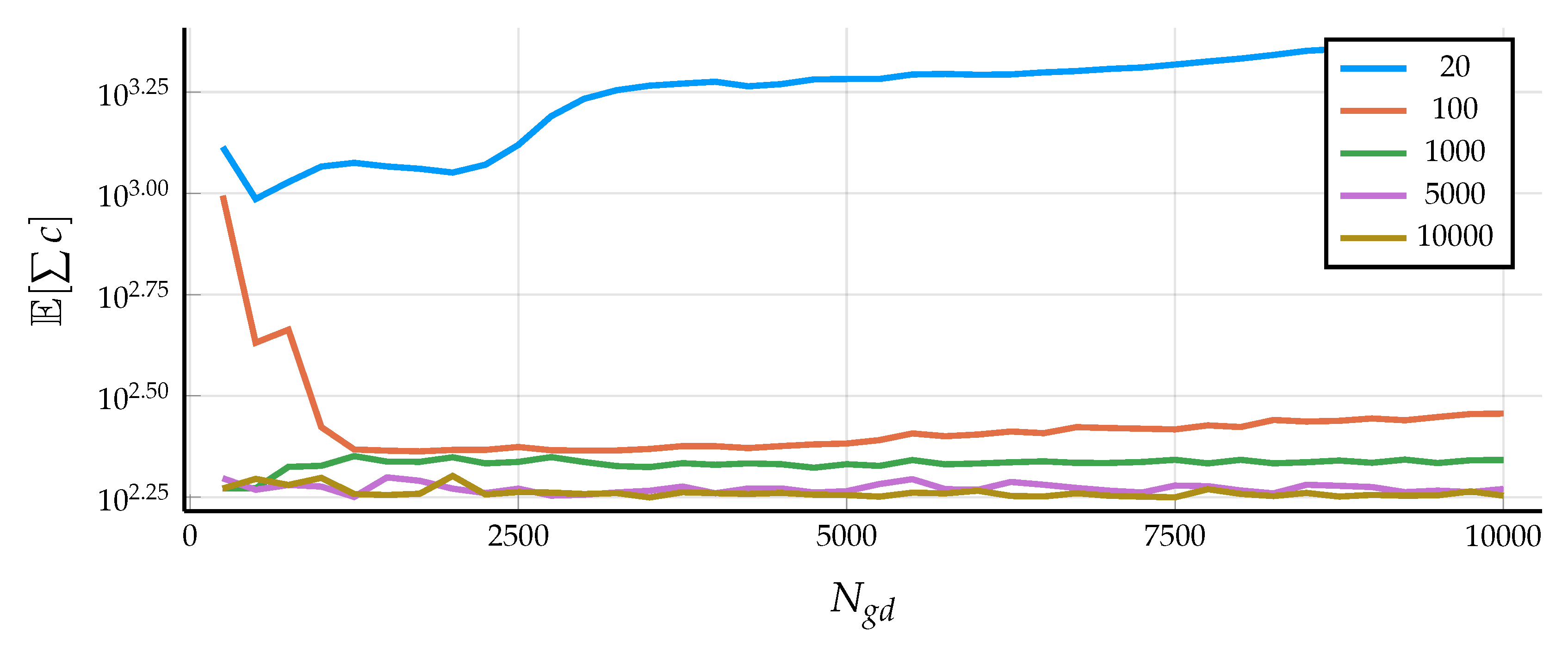
As a first analysis, the influence of the number of trajectories and the number of training epochs on the performance on the oracle network is analyzed. Figure 3 shows the expected value of accumulated costs J E , c of oracle controllers, trained by supervised learning on a different number of trajectories N for different numbers of epochs N g d . For a small number of trajectories N, the best control performance is reached after a few epochs of supervised learning and the performance starts degrading with more training. Thus, a decrease in the error during supervised learning does not necessarily lead to an increase in the closed-loop performance. Including more trajectories leads to an increased performance in the closed loop. Including more than 5000 trajectories, however, did not lead to a noticeable increase in the closed loop performance for our case. The only case that produced a controller unable to stabilize the system was with as low as 20 trajectories.
We use the oracle controller that uses all 10000 trajectories to train our recurrent controller r ( x , h ) using DOI. The mean simulation costs of the recurrent controller is depicted in Figure 4, computed every 5 training episodes. The costs are decreasing exponentially with the number of training episodes in our case.
For each type of controller, i.e., static, oracle, recurrent and adaptive recurrent controllers, we extract the controllers with the best average closed loop performance that we obtained in the training on 10,000 trajectories for the following comparison. We evaluate the metrics in Equations (16)–(19b) on the test-set of 2000 initial states and model parameters. The values for each controller are shown in Table 2. The oracle network slightly outperforms the simple controller without parameter information in terms of mean costs and maximum above optimal costs. The recurrent controller performs better even than the oracle network in terms of both mean costs and maximal above optimal costs. For the mean accumulated costs this is unexpected, as the recurrent controller did not have a direct access to the cost function during its training. For the maximum above optimal accumulated costs, we believe that the recurrent layer is able to average out poor actions in individual states by acting on the past history instead of only acting on the current state. The adjustable controllers do not perform as well as the non-adjustable controllers in terms of mean costs for the case λ = 0 . Also, for the adjustable case the recurrent controller outperforms the static controller with regards to J max , c .

5.3. Control Performance in the Application

The controllers, trained in simulation, are transferred unchanged to the real system. To evaluate the control performance, we record measurements of each controller for a test trajectory and evaluate the costs in Equation (13). Our test trajectory is 220 s long and contains 10 random target locations. Every 10 s, the target location changes from the origin to one of the target locations and then back to the origin after another 10 s. The accumulated costs over our test trajectory, i.e., t c x ( x t ) and t c u ( u t ) , for different controllers are given in Table 3 with lower values indicating a better control performance. The recurrent controllers r ( x , h ) and r λ ( x , 0 , h ) , trained on various model dynamics, achieve a better performance than the static controller with accumulated costs reduced by 20 % and 22.7 % . The controller r λ ( x , 0.3 , h ) is also represented in the table, and performs slightly worse than r λ ( x , 0 , h ) . This is expected as the cost functions (13a) that is used for the evaluation of the values in Table 3 is different from the costs in Equation (15) for λ 0 .
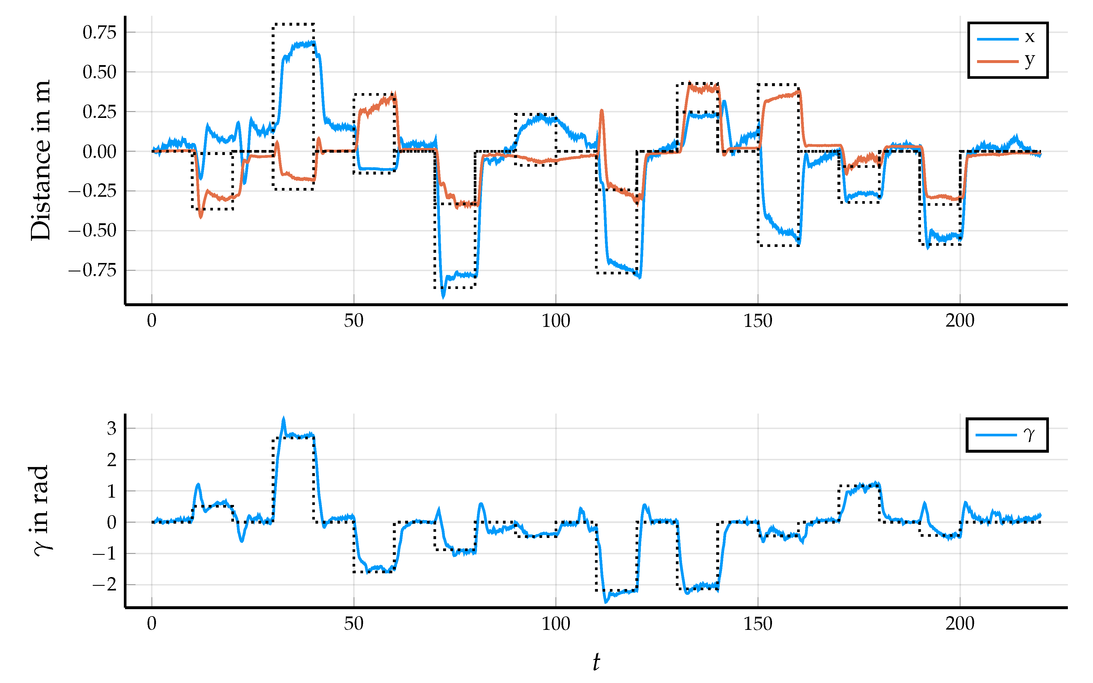
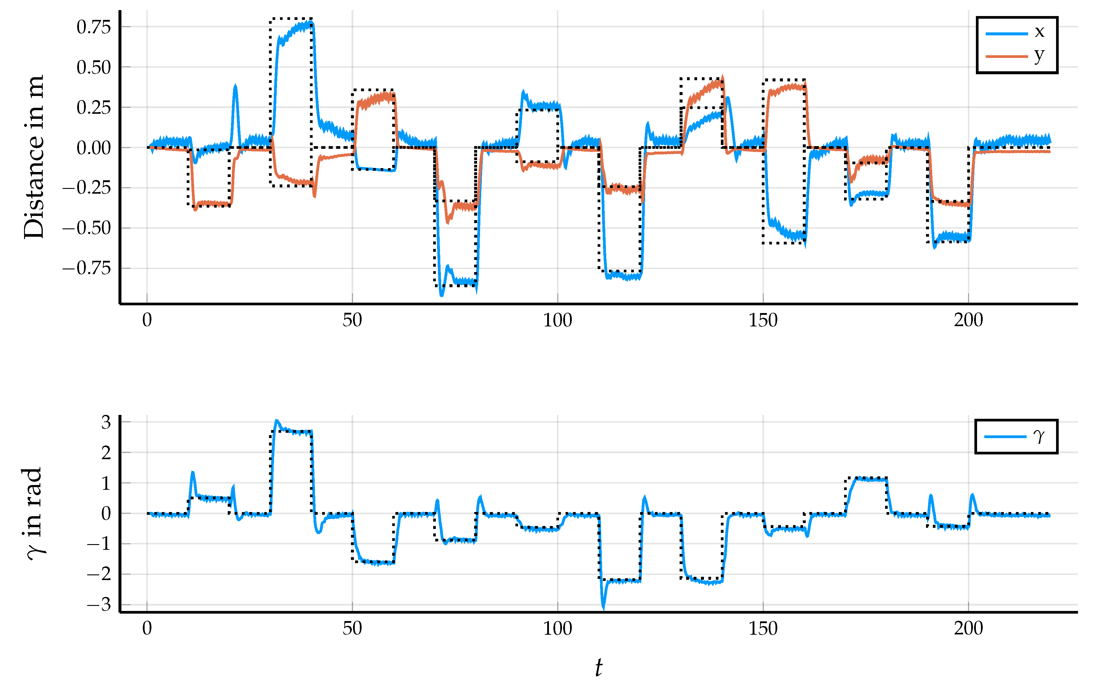
Measurement data for the test trajectory for the static controller g ( x ) , the recurrent controller r ( x , h ) and the adjusted controller r λ ( x , 0.3 , h ) are shown in Figure 5, Figure 6 and Figure 7, respectively. In the application, the approaching of the target position is slower than in simulation due to oscillations in the tilt angle at low velocities. The remaining position error is most pronounced for the static controller in Figure 5, e.g., when approaching the new target position after 30 s. The position error is visibly reduced using a recurrent controller r ( x , h ) as can be seen comparing Figure 6 with Figure 5. The performance increase is also reflected in a reduced value for t c x in Table 3. However, even after 10 s the target location is not reliably reached for the static and the recurrent controller, as the controllers try to reduce the angular velocity of the tilt angle rather than drive towards the target position. We therefore use the adjustable controller r λ ( x , λ , h ) and increase the adjusting parameter λ to give more weight to the position and less weight to velocities. As can be seen in Table 3, this leads to an increase in the accumulated costs compared to the controller r ( x , h ) according to the cost function in Equation (13), caused by higher velocities and control signals. However, the behavior is subjectively better due to faster and more accurate approaching of the target location as is seen in Figure 7. Increasing λ also increases the speed of convergence and accuracy of the yaw angle, as can be seen by comparing Figure 7 with Figure 5 and Figure 6 respectively.
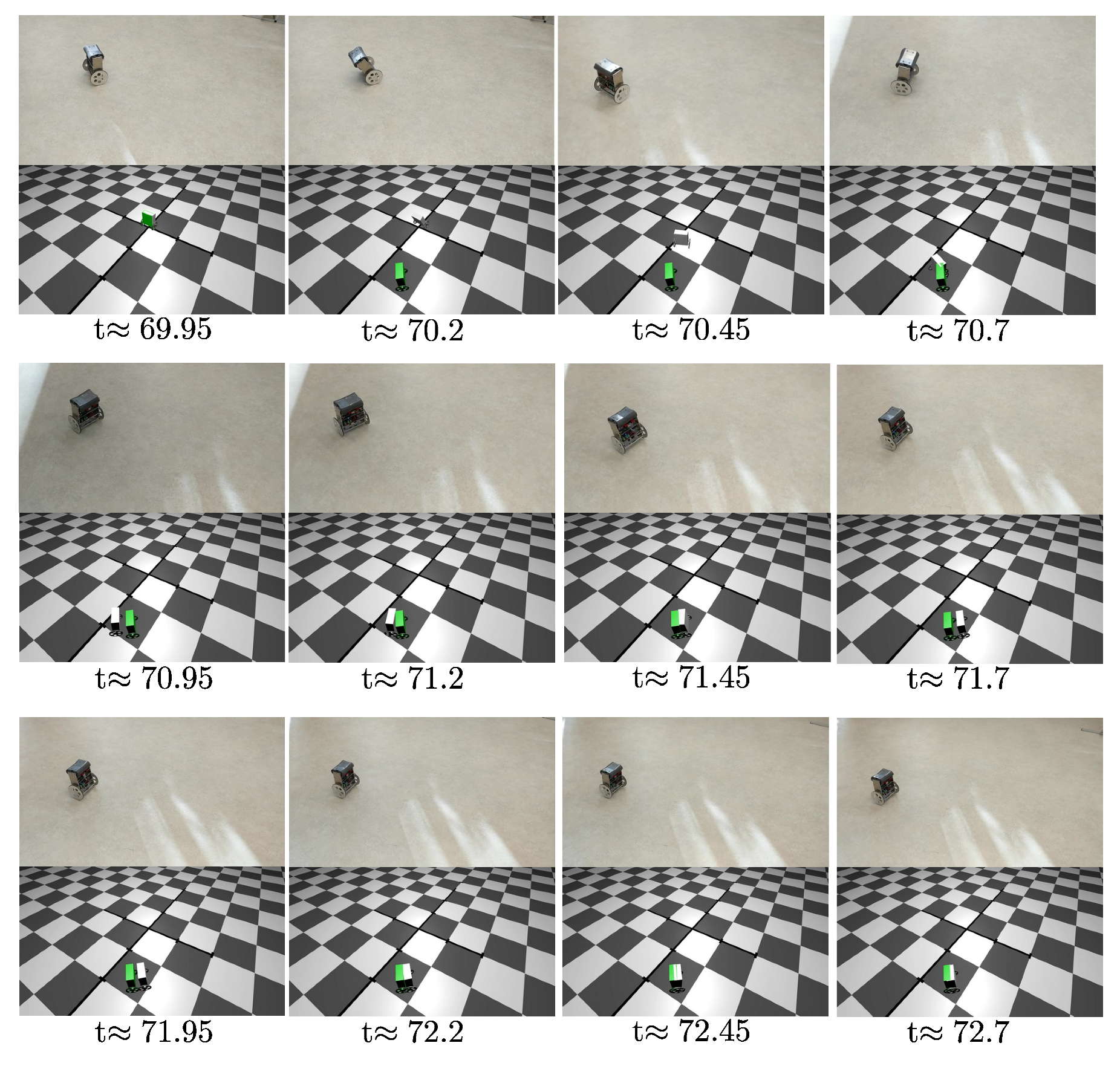
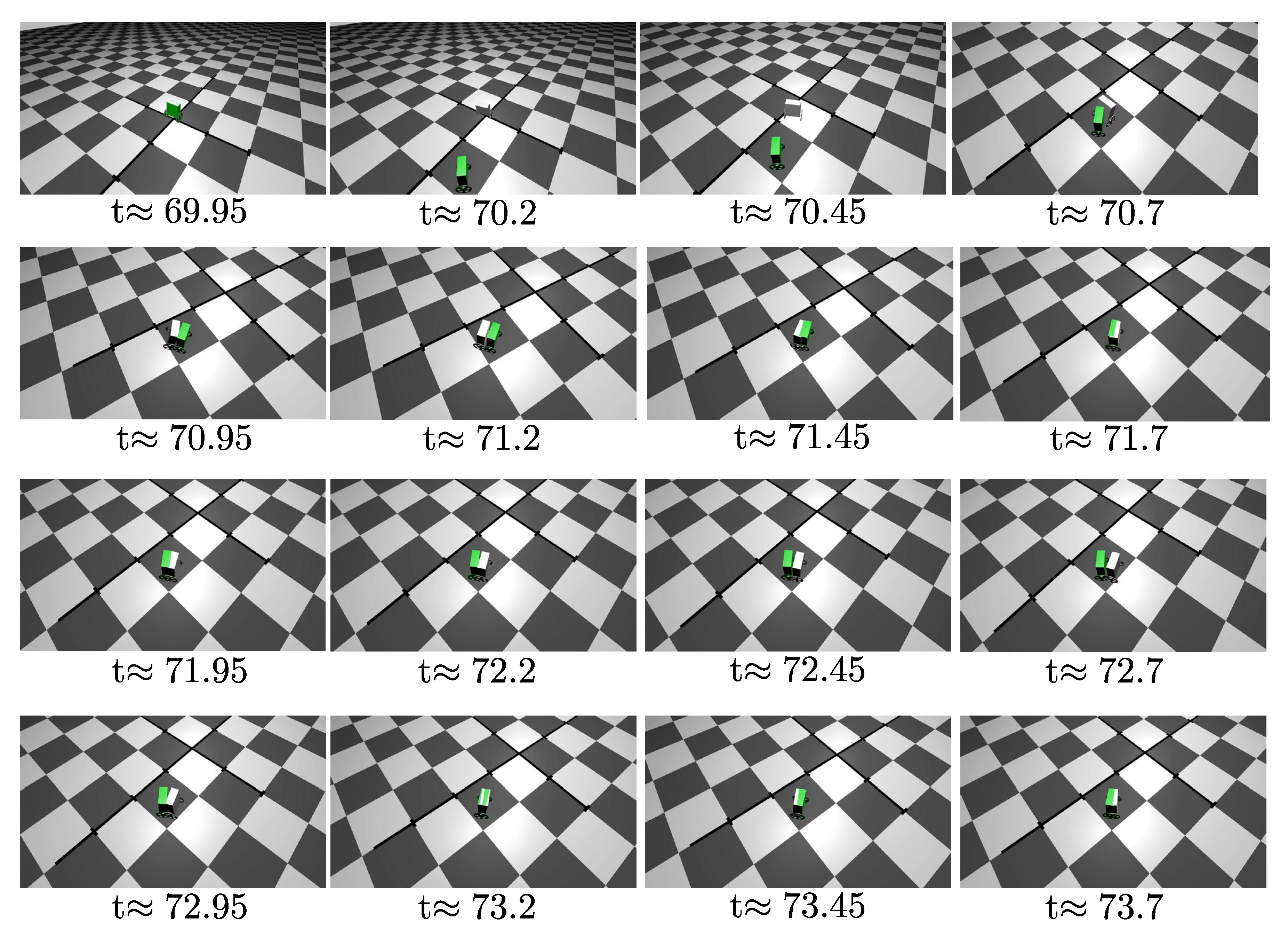
For a qualitative impression of the control performance of the final controller r λ ( x , λ , h ) with λ = 0.3 , a sequence of images of the MIP during the test trajectory is shown in Figure 8 for the real application and in Figure 9 for the same controller in the simulation. For the real application, a visualisation of the recorded measurement data is provided for each timestep as well, with the target position depicted as a static green MIP. The time delay between each image is 0.25 s. Comparing both, we see that the dynamic manoeuvre is performed almost identically with the largest differences close to the position of rest. For a further qualitative impression, a video of the MIP using the adjustable controller is accessible at https://youtu.be/MwVZgRJSnXg.

5.4. Outlook of Application Specific Variations

Our controller was trained to drive the MIP towards static target positions and orientations. By continuously shifting the target position, a trajectory or a moving target can be followed by this type of controller as well. An application suited for this type of controller is, e.g., driving after a person based on an on-board camera. However, the MIP will be driving slightly behind the target position in the case of a moving target, as it was trained to reach targets with zero velocity. This effect can be seen in the video at https://youtu.be/MwVZgRJSnXg. If a more precise trajectory tracking is required, one has to include training data of trajectories that were optimized to follow non stationary targets. Other tasks, e.g., ascending slopes or avoiding collisions, also require the addition of optimized trajectories specific for that task.

6. Conclusions

We developed a parametric feedback controller for the mobile inverted pendulum using imitation learning with optimized trajectories. The controller is able to stabilize the system and drive to target positions within a certain radius without the need to compute trajectories online. The optimal trajectories used in the training were generated using varying model parameters in simulation and the controller used a recurrent structure in order to adapt its behavior to the real system. In order to train a recurrent controller using imitation learning, it is necessary to have training targets on state sequences generated by the recurrent controller itself. We therefore trained an intermediate oracle controller with full information of the model parameters that acts as a teacher to the recurrent controller. We show an improvement of the robustness of the controller both in simulation and in the real application by comparing it to a controller without the recurrent structure. Finally, an additional input allows us to easily adjust the behavior of the recurrent controller in the application.

Author Contributions

Conceptualization, methodology, software, validation, formal analysis, investigation, data curation, writing—original draft preparation, visualization: C.D.; resources, writing—review and editing, supervision, project administration, funding acquisition: B.L. All authors have read and agreed to the published version of the manuscript.

Funding

This research was partially funded by the German Research Foundation DFG, SFB768.

Conflicts of Interest

The authors declare no conflict of interest.

Abbreviations

The following abbreviations are used in this manuscript:
DAGGERDataset aggregation
DARTDisturbances for augmenting robot trajectories
DOIDisturbed oracle imitation
MIPMobile inverted pendulum
MPCModel Predictive Control
TBPTTTruncated backpropagation through time

Appendix A. Rigid Body Dynamics Model

The rigid body dynamics model of a MIP that is derived in Pathak et al. [47] is repeated in the following. The input is a vector of torques applied to the right and left wheels τ = [ τ r , τ l ] . The model parameters with description are depicted in Table 1. The state space model is
x ˙ = cos ( α ) · v
y ˙ = sin ( α ) · v
γ ˙ = γ ˙
α ˙ = α ˙
α ¨ = f 5 ( x ) + g 5 ( x ) ( τ r + τ l )
v ˙ = f 6 ( x ) + g 6 ( x ) ( τ r + τ l )
γ ¨ = f 7 ( x ) + g 7 ( x ) ( τ r τ l )
with the abbreviations
D ( α ) = M b 2 cos 2 ( α ) c z R 2 + ( M b 2 2 M w M b ) c z 2 2 I y y M w I y y M b R 2 2 M b c z 2 I w a 2 I y y I w a
G ( α ) = ( M b c z 2 + I z z I x x ) R 2 cos 2 ( α ) + ( M b c z 2 + I x x + 2 I w d + 2 b 2 M w ) R 2 + 2 b 2 I w a
K ( α ) = M b R 2 c z sin ( α ) 4 I y y 3 M b c z 2 + I x x I z z + M b R 2 c z sin ( 3 α ) I x x I z z + M b c z 2
H = 1 2 M b R 2 + M w R 2 + I w a ( I z z I x x ) M b c z 2 ( M w R 2 + I w a )
f 5 ( x ) = sin ( 2 α ) γ ˙ 2 H M b c z g sin ( α ) M b R 2 + 2 ( I w a + M w R 2 ) D ( α ) + M b 2 c z 2 R 2 sin ( 2 α ) α ˙ 2 2 D ( α )
f 6 ( x ) = K ( α ) γ ˙ 2 + M b 2 c z 2 R 2 g sin ( 2 α ) 2 sin ( α ) α ˙ 2 M b R 2 c z I y y + M b c z 2 2 D ( α )
f 7 ( x ) = R 2 γ ˙ G ( α ) sin ( 2 α ) α ˙ ( I x x I z z + M b c z 2 ) + sin ( α ) M b c z v
g 5 ( x ) = M b R 2 + 2 M w R 2 + 2 I w a + M b cos ( α ) c z R D ( α )
g 6 ( x ) = R M b cos ( α ) c z R + I y y + M b c z 2 D ( α )
g 7 ( x ) = R b G ( α ) .

References

  1. Yang, C.; Li, Z.; Li, J. Trajectory planning and optimized adaptive control for a class of wheeled inverted pendulum vehicle models. IEEE Trans. Cybern. 2012, 43, 24–36. [Google Scholar] [CrossRef] [PubMed] [Green Version]
  2. Schulman, J.; Wolski, F.; Dhariwal, P.; Radford, A.; Klimov, O. Proximal Policy Optimization Algorithms. arXiv 2017, arXiv:1707.06347. [Google Scholar]
  3. Faulwasser, T.; Weber, T.; Zometa, P.; Findeisen, R. Implementation of nonlinear model predictive path-following control for an industrial robot. IEEE Trans. Control Syst. Technol. 2016, 25, 1505–1511. [Google Scholar] [CrossRef] [Green Version]
  4. Deisenroth, M.; Rasmussen, C.E. PILCO: A model-based and data-efficient approach to policy search. In Proceedings of the 28th International Conference on Machine Learning (ICML-11), Bellevue, WA, USA, 28 June–2 July 2011; pp. 465–472. [Google Scholar]
  5. Golemo, F.; Taiga, A.A.; Courville, A.; Oudeyer, P.Y. Sim-to-Real Transfer with Neural-Augmented Robot Simulation. In Proceedings of the Conference on Robot Learning, Zurich, Switzerland, 29–31 October 2018; pp. 817–828. [Google Scholar]
  6. Pattanaik, A.; Tang, Z.; Liu, S.; Bommannan, G.; Chowdhary, G. Robust deep reinforcement learning with adversarial attacks. In Proceedings of the 17th International Conference on Autonomous Agents and MultiAgent Systems, Stockholm, Sweden, 10–15 July 2018; pp. 2040–2042. [Google Scholar]
  7. Pinto, L.; Davidson, J.; Sukthankar, R.; Gupta, A. Robust adversarial reinforcement learning. arXiv 2017, arXiv:1703.02702. [Google Scholar]
  8. Rajeswaran, A.; Ghotra, S.; Ravindran, B.; Levine, S. Epopt: Learning robust neural network policies using model ensembles. arXiv 2016, arXiv:1610.01283. [Google Scholar]
  9. Peng, X.B.; Andrychowicz, M.; Zaremba, W.; Abbeel, P. Sim-to-real transfer of robotic control with dynamics randomization. In Proceedings of the 2018 IEEE International Conference on Robotics and Automation (ICRA), Brisbane, Australia, 21–25 May 2018; pp. 1–8. [Google Scholar]
  10. Muratore, F.; Treede, F.; Gienger, M.; Peters, J. Domain randomization for simulation-based policy optimization with transferability assessment. In Proceedings of the Conference on Robot Learning, Zurich, Switzerland, 29–31 October 2018; pp. 700–713. [Google Scholar]
  11. Hussein, A.; Gaber, M.M.; Elyan, E.; Jayne, C. Imitation learning: A survey of learning methods. ACM Comput. Surv. (CSUR) 2017, 50, 21. [Google Scholar] [CrossRef]
  12. Dessort, R.; Chucholowski, C. Explicit model predictive control of semi-active suspension systems using Artificial Neural Networks (ANN). In 8th International Munich Chassis Symposium 2017; Pfeffer, P.E., Ed.; Springer Fachmedien Wiesbaden: Wiesbaden, Germany, 2017; pp. 207–228. [Google Scholar]
  13. Mordatch, I.; Todorov, E. Combining the benefits of function approximation and trajectory optimization. Robot. Sci. Syst. 2014, 4, 5–32. [Google Scholar]
  14. Abbeel, P.; Quigley, M.; Ng, A.Y. Using inaccurate models in reinforcement learning. In Proceedings of the 23rd International Conference on Machine Learning, Pittsburgh, PA, USA, 25–29 June 2006; pp. 1–8. [Google Scholar]
  15. Mordatch, I.; Lowrey, K.; Todorov, E. Ensemble-CIO: Full-body dynamic motion planning that transfers to physical humanoids. In Proceedings of the 2015 IEEE/RSJ International Conference on Intelligent Robots and Systems (IROS), Hamburg, Germany, 28 September–2 October 2015; pp. 5307–5314. [Google Scholar]
  16. Liu, C.; Li, H.; Gao, J.; Xu, D. Robust self-triggered min–max model predictive control for discrete-time nonlinear systems. Automatica 2018, 89, 333–339. [Google Scholar] [CrossRef]
  17. Yu, W.; Liu, C.K.; Turk, G. Preparing for the Unknown: Learning a Universal Policy with Online System Identification. arXiv 2017, arXiv:1702.02453. [Google Scholar]
  18. Schulman, J.; Levine, S.; Moritz, P.; Jordan, M.I.; Abbeel, P. Trust Region Policy Optimization. arXiv 2015, arXiv:1502.05477. [Google Scholar]
  19. Muratore, F.; Gienger, M.; Peters, J. Assessing Transferability from Simulation to Reality for Reinforcement Learning. IEEE Trans. Pattern Anal. Mach. Intell. 2019. [Google Scholar] [CrossRef] [Green Version]
  20. Bousmalis, K.; Irpan, A.; Wohlhart, P.; Bai, Y.; Kelcey, M.; Kalakrishnan, M.; Downs, L.; Ibarz, J.; Pastor, P.; Konolige, K.; et al. Using simulation and domain adaptation to improve efficiency of deep robotic grasping. In Proceedings of the 2018 IEEE International Conference on Robotics and Automation (ICRA), Brisbane, Australia, 21–25 May 2018; pp. 4243–4250. [Google Scholar]
  21. Chebotar, Y.; Handa, A.; Makoviychuk, V.; Macklin, M.; Issac, J.; Ratliff, N.; Fox, D. Closing the sim-to-real loop: Adapting simulation randomization with real world experience. In Proceedings of the 2019 International Conference on Robotics and Automation (ICRA), Montreal, QC, Canada, 20–24 May 2019; pp. 8973–8979. [Google Scholar]
  22. Salimans, T.; Ho, J.; Chen, X.; Sutskever, I. Evolution strategies as a scalable alternative to reinforcement learning. arXiv 2017, arXiv:1703.03864. [Google Scholar]
  23. Chrabaszcz, P.; Loshchilov, I.; Hutter, F. Back to Basics: Benchmarking Canonical Evolution Strategies for Playing Atari. arXiv 2018, arXiv:1802.08842. [Google Scholar]
  24. Rückstieß, T.; Sehnke, F.; Schaul, T.; Wierstra, D.; Sun, Y.; Schmidhuber, J. Exploring parameter space in reinforcement learning. Paladyn 2010, 1, 14–24. [Google Scholar] [CrossRef]
  25. Ortega, J.G.; Camacho, E. Mobile robot navigation in a partially structured static environment, using neural predictive control. Control Eng. Pract. 1996, 4, 1669–1679. [Google Scholar] [CrossRef]
  26. Åkesson, B.M.; Toivonen, H.T.; Waller, J.B.; Nyström, R.H. Neural network approximation of a nonlinear model predictive controller applied to a pH neutralization process. Comput. Chem. Eng. 2005, 29, 323–335. [Google Scholar] [CrossRef]
  27. Ross, S.; Gordon, G.; Bagnell, D. A reduction of imitation learning and structured prediction to no-regret online learning. In Proceedings of the Fourteenth International Conference on Artificial Intelligence and Statistics, Ft. Lauderdale, FL, USA, 11–13 April 2011; pp. 627–635. [Google Scholar]
  28. He, H.; Eisner, J.; Daume, H. Imitation learning by coaching. In Advances in Neural Information Processing Systems; Curran Associates, Inc.: Red Hook, NY, USA, 2012; pp. 3149–3157. [Google Scholar]
  29. Laskey, M.; Lee, J.; Fox, R.; Dragan, A.; Goldberg, K. Dart: Noise injection for robust imitation learning. arXiv 2017, arXiv:1703.09327. [Google Scholar]
  30. Mordatch, I.; Lowrey, K.; Andrew, G.; Popovic, Z.; Todorov, E.V. Interactive control of diverse complex characters with neural networks. In Advances in Neural Information Processing Systems; Curran Associates, Inc.: Red Hook, NY, USA, 2015; pp. 3132–3140. [Google Scholar]
  31. Levine, S.; Koltun, V. Guided policy search. In Proceedings of the 30th International Conference on Machine Learning (ICML-13), Atlanta, GA, USA, 16–21 June 2013; pp. 1–9. [Google Scholar]
  32. Levine, S.; Koltun, V. Learning complex neural network policies with trajectory optimization. In Proceedings of the International Conference on Machine Learning, Bejing, China, 22–24 June 2014; pp. 829–837. [Google Scholar]
  33. Zhang, T.; Kahn, G.; Levine, S.; Abbeel, P. Learning deep control policies for autonomous aerial vehicles with mpc-guided policy search. In Proceedings of the 2016 IEEE international conference on robotics and automation (ICRA), Stockholm, Sweden, 16–21 May 2016; pp. 528–535. [Google Scholar]
  34. Kahn, G.; Zhang, T.; Levine, S.; Abbeel, P. PLATO: Policy Learning using Adaptive Trajectory Optimization. In Proceedings of the 2017 IEEE International Conference on Robotics and Automation (ICRA), Singapore, 29 May–3 June 2017. [Google Scholar]
  35. Levine, S.; Finn, C.; Darrell, T.; Abbeel, P. End-to-end training of deep visuomotor policies. J. Mach. Learn. Res. 2016, 17, 1334–1373. [Google Scholar]
  36. Paul, S.; Kurin, V.; Whiteson, S. Fast Efficient Hyperparameter Tuning for Policy Gradient Methods. In Advances in Neural Information Processing Systems; Curran Associates, Inc.: Red Hook, NY, USA, 2019; pp. 4618–4628. [Google Scholar]
  37. Von Stryk, O.; Bulirsch, R. Direct and indirect methods for trajectory optimization. Ann. Oper. Res. 1992, 37, 357–373. [Google Scholar] [CrossRef]
  38. Bock, H.G.; Plitt, K.J. A multiple shooting algorithm for direct solution of optimal control problems. IFAC Proc. Vol. 1984, 17, 1603–1608. [Google Scholar] [CrossRef]
  39. Biegler, L.T. Nonlinear Programming: Concepts, Algorithms, and Applications to Chemical Processes; SIAM: Philadelphia, PA, USA, 2010; Volume 10. [Google Scholar]
  40. Wächter, A. An Interior Point Algorithm for Large-Scale Nonlinear Optimization with Applications in Process Engineering. Ph.D. Thesis, Carnegie Mellon University, Pittsburgh, PA, USA, 2002. [Google Scholar]
  41. Kingma, D.P.; Ba, J. Adam: A Method for Stochastic Optimization. arXiv 2014, arXiv:1412.6980. [Google Scholar]
  42. Tallec, C.; Ollivier, Y. Unbiasing Truncated Backpropagation Through Time. arXiv 2017, arXiv:1705.08209. [Google Scholar]
  43. Ang, K.H.; Chong, G.; Li, Y. PID control system analysis, design, and technology. IEEE Trans. Control Syst. Technol. 2005, 13, 559–576. [Google Scholar]
  44. Muralidharan, V.; Mahindrakar, A.D. Position Stabilization and Waypoint Tracking Control of Mobile Inverted Pendulum Robot. IEEE Trans. Control Syst. Technol. 2014, 22, 2360–2367. [Google Scholar] [CrossRef]
  45. Dini, N.; Majd, V.J. Model predictive control of a wheeled inverted pendulum robot. In Proceedings of the 2015 3rd RSI International Conference on Robotics and Mechatronics (ICROM), Tehran, Iran, 7–9 October 2015; pp. 152–157. [Google Scholar] [CrossRef]
  46. Ha, J.; Lee, J. Position control of mobile two wheeled inverted pendulum robot by sliding mode control. In Proceedings of the 2012 12th International Conference on Control, Automation and Systems, JeJu Island, Korea, 17–21 October 2012; pp. 715–719. [Google Scholar]
  47. Pathak, K.; Franch, J.; Agrawal, S.K. Velocity and position control of a wheeled inverted pendulum by partial feedback linearization. IEEE Trans. Robot. 2005, 21, 505–513. [Google Scholar] [CrossRef]
  48. Kara, T.; Eker, I. Nonlinear modeling and identification of a DC motor for bidirectional operation with real time experiments. Energy Convers. Manag. 2004, 45, 1087–1106. [Google Scholar] [CrossRef]
  49. Achiam, J.; Held, D.; Tamar, A.; Abbeel, P. Constrained Policy Optimization. In Proceedings of the 34th International Conference on Machine Learning, Sydney, Australia, 6–11 August 2017. [Google Scholar]
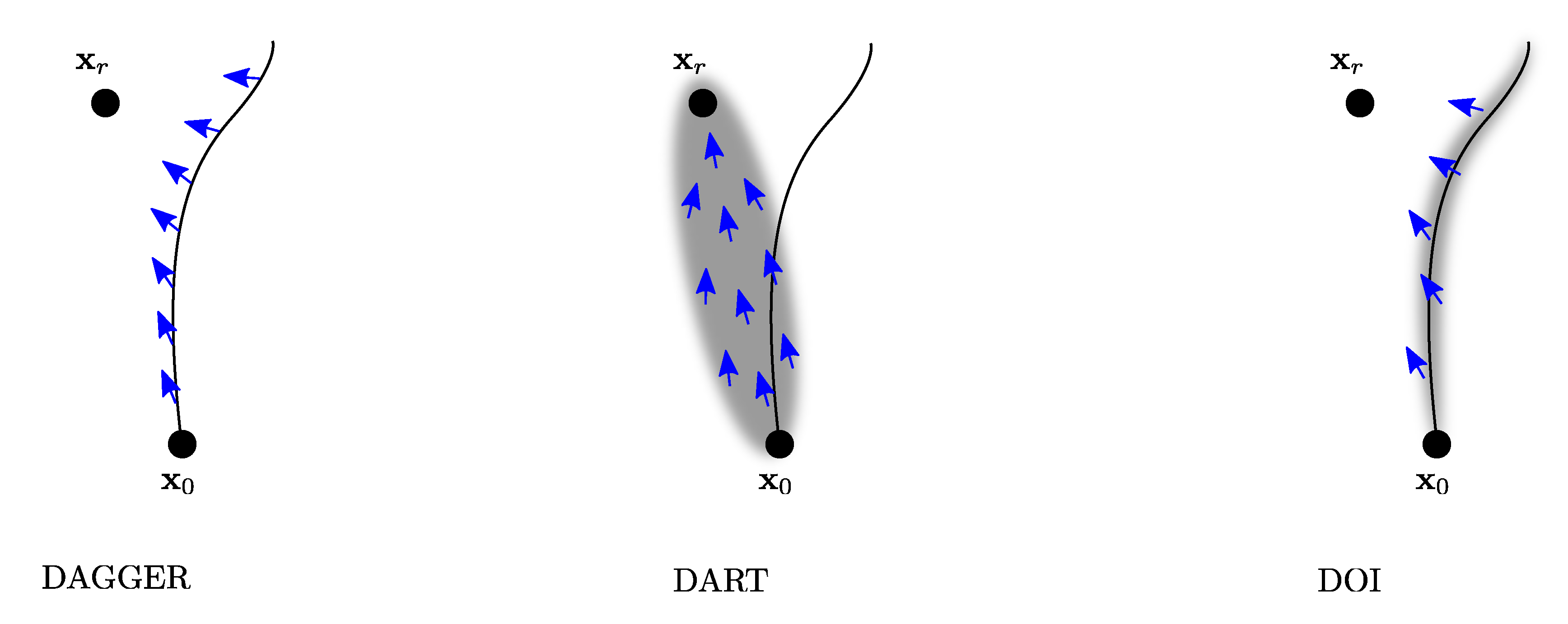
Figure 1. Visual comparison of DAGGER, DART and DOI. x 0 inidicates the intial state and x r a reference state with low costs. The black line indicates a trajectory sampled using the parametric controller in the loop. Blue arrows indicate the training data created for each approach, possibly generated for a distribution of trajectories, indicated by a blurred area.
Robotics 09 00029 g001
Figure 2. The mobile inverted pendulum (MIP).
Robotics 09 00029 g002
Figure 3. Mean accumulated costs of oracle controllers g ( x , p ) trained on different numbers of trajectories over N e p o c h epochs. The number of trajectories used during training is given in the line label.
Robotics 09 00029 g003
Figure 4. Mean accumulated costs of the recurrent controller r ( x , h ) trained using DOI over the number of epochs N e p o c h .
Robotics 09 00029 g004
Figure 5. Measurement data for an application of a static neural network controller g ( x ) . Units are in meters for the position coordinates x and y (top plot) and radian for γ (bottom plot).
Robotics 09 00029 g005
Figure 6. Measurement data for an application of a recurrent neural network controller r ( x , h ) . Units are in meters for the position coordinates x and y (top plot) and radian for γ (bottom plot).
Robotics 09 00029 g006
Figure 7. Measurement data for an application of an adjustable recurrent neural network controller r λ ( x , λ , h ) with λ = 0.3 . Units are in meters for the position coordinates x and y (top plot) and radian for γ (bottom plot).
Robotics 09 00029 g007
Figure 8. Image sequence showing a manoeuvre of the real MIP using the recurrent control structure r λ ( x , λ , h ) with λ = 0.3 . The top image shows the real system and attached below is a visualization of the measurement data (gray MIP), also showing the target position as a green MIP.
Robotics 09 00029 g008
Figure 9. Image sequence showing a manoeuvre of the MIP in simulation using the recurrent control structure r λ ( x , λ , h ) with λ = 0.3 . The target position is shown as a green MIP.
Robotics 09 00029 g009
Table 1. Model parameters of the mobile inverted pendulum.
VariableValueUnitDescription
M b 1.76 kg Mass of the body
M w 0.147 kg Mass of a wheel
R0.07 m Radius of the wheels
c z 0.07 ± 20 % m Height of the center of mass above wheel axis
b0.09925 m Half length between wheels
I x x 0.0191 k g   m 2 Moment of inertia, x-axis
I y y 0.0158 ± 20 % k g   m 2 Moment of inertia, y-axis
I z z 0.0048 k g   m 2 Moment of inertia, z-axis
I w a 3.6 · 10 4 k g   m 2 Moment of inertia. Wheel, y-axis
I w d 1.45 · 10 3 k g   m 2 Moment of inertia. Wheel, z-axis
k 1 0.018 V s Motor constant
k 2 0.61 N   m   A 1 Motor constant
c fric , 1 0.24 ± 20 % N   m 1 Friction model constant
c fric , 2 2.0/Friction model constant
c fric , 3 0.4/Friction model constant
c fric , 4 8 · 10 4 N   s   m 1 Friction model constant
Table 2. Mean and maximal accumulated costs for different controllers in simulation. Controllers with gray font can not be used in practice and are only given as a reference.
g ( x ) g ( x , p ) r ( x , h ) g λ ( x , 0 , p ) r λ ( x , 0 , h ) opt.
J E , c 181.47178.33176.58185.81185.75155.163
J max , c 712.03520.95121.38494.27182.670
J E , c T 0.1330.1020.0900.0700.0510
J max , c T 1.102.131.341.0920.5240
Table 3. Accumulated costs for different controllers on a test trajectory in the real application .
g ( x ) r ( x , h ) r λ ( x , 0 , h ) r λ ( x , 0.3 , h )
c x 5221.863957.264062.044131.76
c u 1674.851566.881265.351431.55
c 6896.715524.145327.395563.31