A Novel Design and Implementation of Autonomous Robotic Car Based on ROS in Indoor Scenario

Abstract

Pervasive deployment of autonomous vehicle all over the world is an undisputed trend in the future. Autonomous vehicle will inevitably play an essential role in decreasing traffic jams, reducing threats from driving while intoxicated (DWI), and assisting the handicapped to get around. At the same time, the new energy vehicles (NEV) especially the electromobile is gradually adopted by several governments like Germany, USA and China as compulsive transportation tools from the standpoint of environmental friendliness. Taking these two crucial trends into consideration, this article proposes a scheme of autonomous robotic car based on robot operation system (ROS) in electromobile-like car which can be easily transplanted to commercial electromobile. In this article, the design and implementation of robotic car are demonstrated in detail which involves overall architecture of functional modules, hardware design, obstacle avoidance, localization and mapping, land detection and tracking, velocity control and indoor navigation. All software modules and hardware are integrated in NVIDIA Jetson TX1 and TRAXXAS car.

1. Introduction

1.1. Background

According to the report from World Health Organization (WHO), around 1.25 million fatalities and 20–50 million injuries each year worldwide were generated due to motor vehicle crashes from 2013 to 2018. In motor vehicle accidents, the 1997 Tri-Level Study of the Causes of Traffic Accidents found that human errors were a definite or probable cause in 90–93% of incidents examined [1]. Statistical data demonstrates that motor vehicle accidents with human error poses a huge threat to human safety. Considering the security, connectivity and convenience of autonomous technology, autonomous techniques are widely studied and deployed worldwide to reduce or even eliminate human errors.

According to the definition of National Highway Traffic Safety Administration (NHTSA) from the US, levels of autonomous vehicle are divided into five stages which respectively are No Automation (Level 0), Function-specific Automation (Level 1), Combined Function Automation (Level 2), Limited Self-Driving Automation (Level 3) and Full Self-Driving Automation (Level 4) [2]. For example, floor mopping robotics belong to Level 1 because they can use the light detection and ranging (liDAR)-based simultaneously localization and mapping (SLAM) algorithm only to navigate themselves and fulfill tasks. Multi-sensor data fusion algorithms can be used in Level-2 robotics, therefore they can combine various sensors and algorithms and fulfill tasks in a robust and accurate way. Multi-sensor data fusion algorithms and other advanced algorithms like reinforcement learning enable robotics to move freely in city scenarios, therefore, these robotics like Tesla Model X belongs to Level 3. The best autonomous robotics up to now belong to Level 3–Level 4. That means that these robotics have been successfully deployed in specific scenarios like city roads, and are expected to be deployed in other complex scenarios. For example, some outstanding companies, such as Tesla, Google and Baidu, have successfully deployed autonomous cars in cities, and these cars are expected to be deployed in suburbs of city or rural areas. On top of achievements from leading corporations, numerous autonomous vehicle schemes from universities or individuals, either motor-based schemes [3,4,5,6,7,8,9,10,11] or electronic-based schemes [12,13,14,15,16,17,18,19], are also extraordinary and have decent performance in various of situations.

1.2. Objectives behind this Article

At the end of 20th century, Japan and USA started to be typical countries in developing the new energy vehicles (NEV)-based automatic industry. Since the early 21st century, the government of Germany, France and China took part in the NEV-based automatic industry and introduced numerous policies to accelerate the development of techniques [20]. Environmental impact and climate change urge governments across the border to prioritize to the development of NEV-based autonomous driving, thereby gradually pushing NEV-based autonomous driving become a prevalent and pervasive trend of future.

Given relevant laws and trends of future in field of autonomous vehicle, this article proposes an electronic-based autonomous vehicle scheme which features the multi-sensor fusion method in obstacle avoidance using convolutional neural network (CNN) and liDAR-based image processing approach. In contrast with traditional approaches, fused approach using deep learning algorithm and liDAR is more precise and robust once sufficient and high-quality dataset are given. Techniques like simultaneously localization and mapping (SLAM), lane detection and tracking, path planning, navigation, data recording and velocity control are also included and successfully tested in the indoor scenario. An intelligent car-like robot is shown in the Figure 1. The Figure 2 represents its test environment in simulated and real-world scenarios respectively.

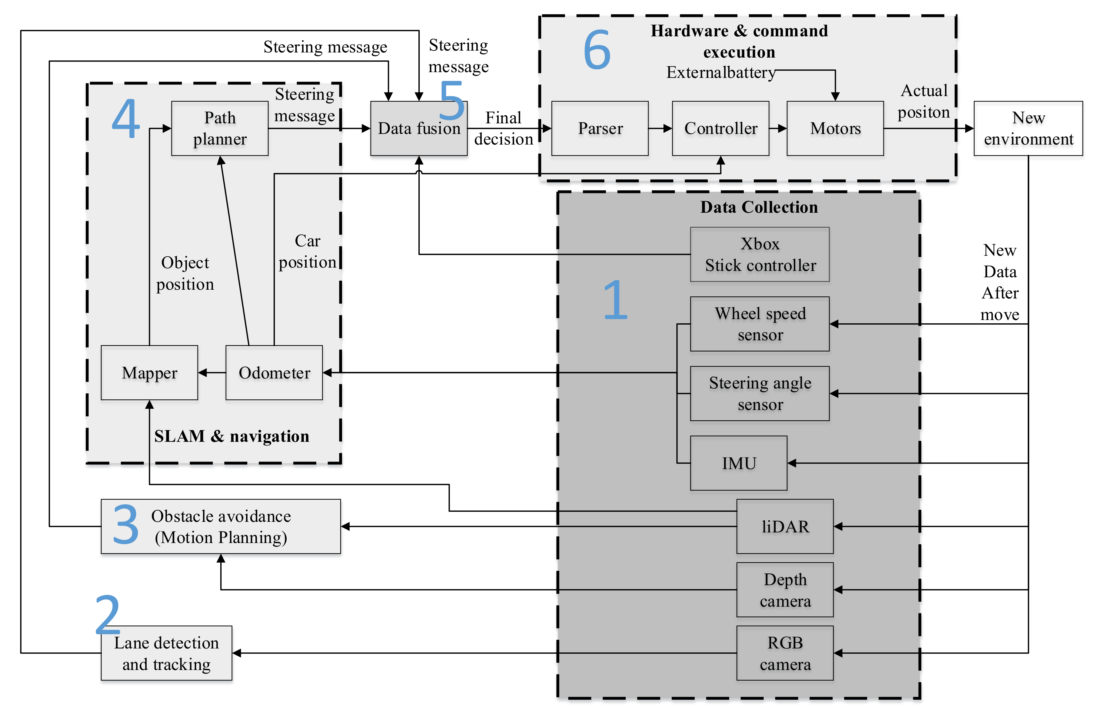
2. Control Loop of Intelligent Autonomous Robotic Car

The architecture of control loop of robotic car can be theoretically divided into six components including sensors (Part 1 in the Figure 3), obstacle avoidance (Part 3 in the Figure 3), lane detection and tracking (Part 2 in the Figure 3), SLAM and navigation (Part 4 in the Figure 3), data fusion (Part 5 in the Figure 3), and command transformation (Part 6 in the Figure 3). The overall control loop of robotic car is demonstrated in the Figure 3.

Various types of raw messages are generated by sensors which include Xbox stick controller, wheel speed sensor, steering angle sensor, inertial measurement unit (IMU), liDAR, depth camera and red-green-blue (RGB) camera. These messages are then sent to the following modules for further processing. To be exact, messages from Xbox stick controller are sent to data fusion module for steering data fusion. Messages generated by wheel speed sensor, steering angle sensor, IMU and liDAR are converted to SLAM and navigation module for pose estimation, path planning and navigation. Depth camera and liDAR provide messages for obstacle avoidance module, while RGB camera generates messages for lane detection and tracking module. In SLAM and navigation module, path planner sub-module receives messages from the mapper where grid-maps are generated using messages from liDAR and odometer, in which messages are from the wheel speed sensor, steering angle sensor and IMU. Eventually, path planner generates steering messages which can be used to generate the steering angle of car. In data fusion module, decision-level data fusion method is adopted to generate ROS-based final decision messages. In command transformation module, ROS-based final decision messages are transformed in parser sub-module to hardware messages that can be recognized and executed by hardware of car in Controller sub-module. Finally, controller processes messages from the parser and odometer to generate final steering angle and speed messages, and drives the car to required positions. New data is then collected from new positions and transmitted to other modules, therefore marking the end of one loop and the start of another loop.

3. Function Modules Design

3.1. Intelligent Obstacle Avoidance System

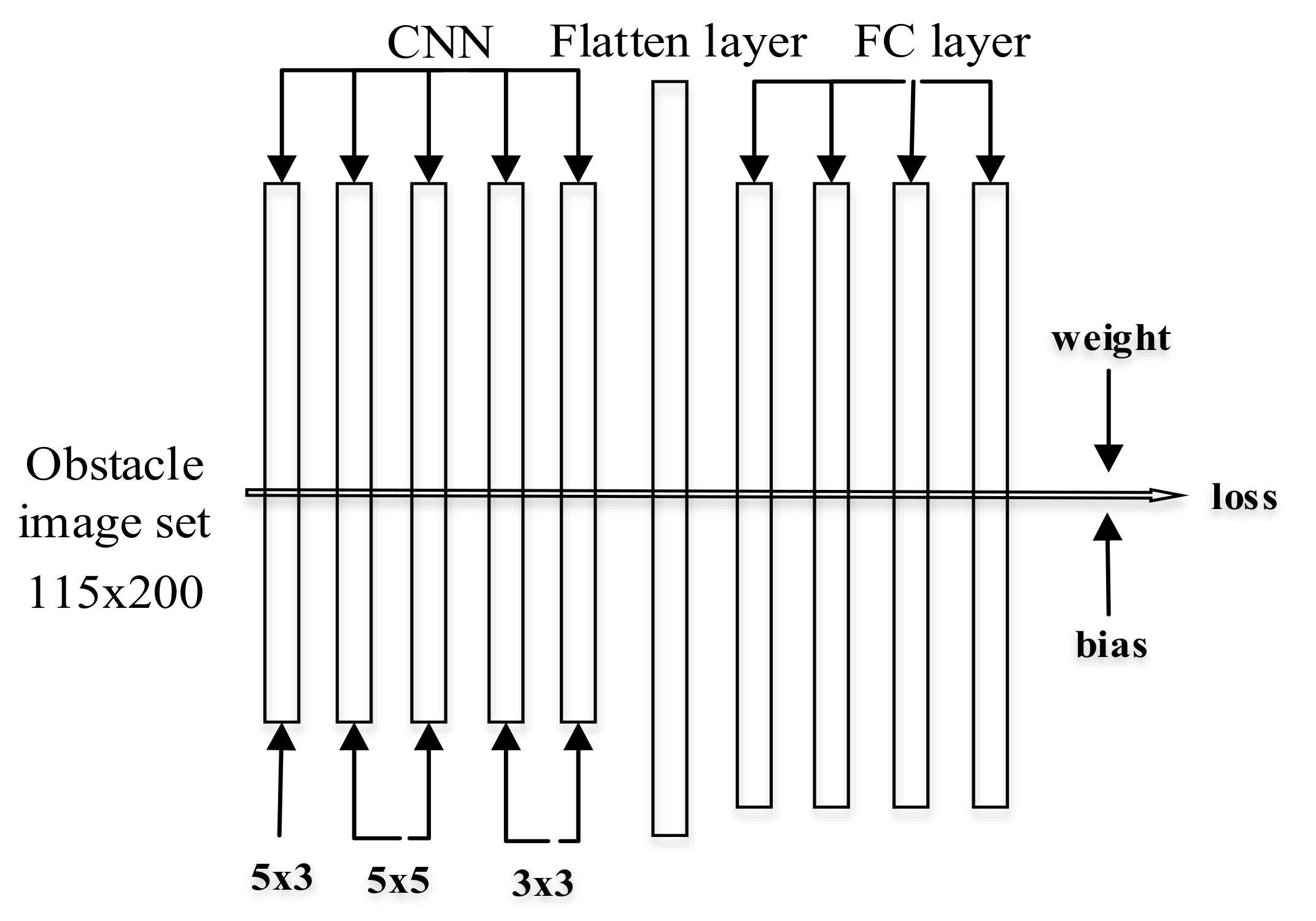
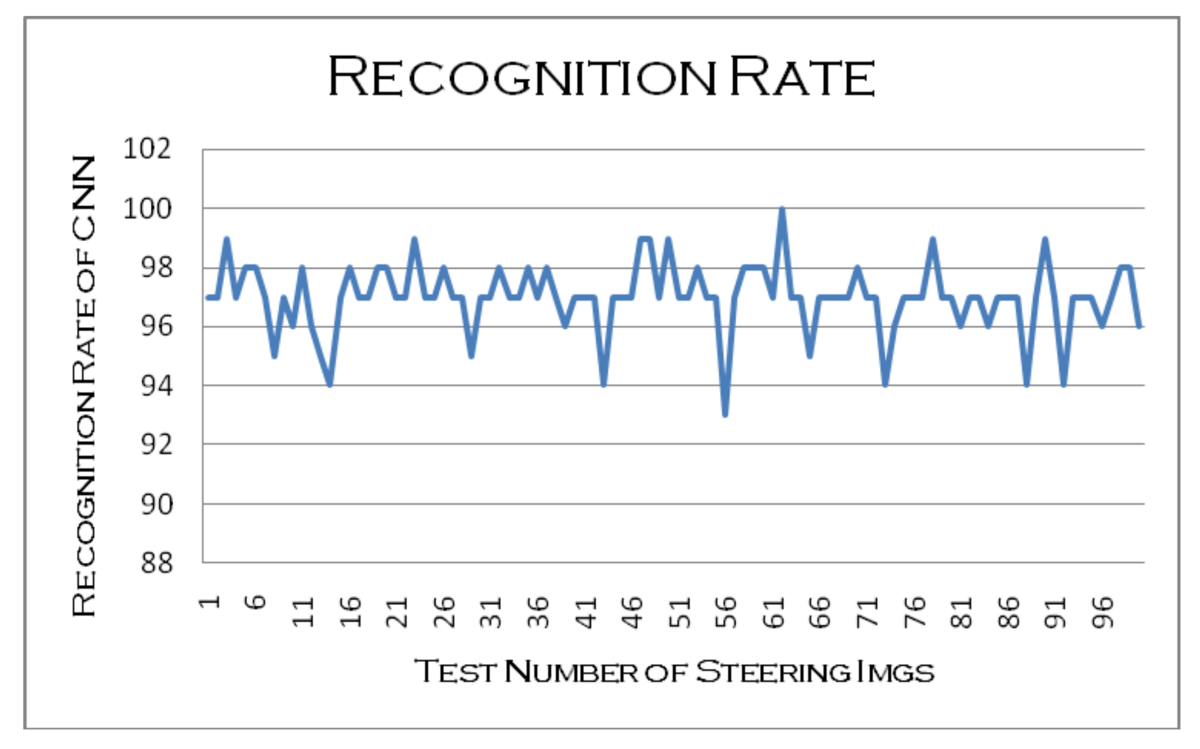
3.1.1. Obstacle Avoidance Based on CNN

There are many contributions based on machine learning and liDAR-based methods for autonomous driving before us. Typical contributions can be found in [21,22]. These methods however are combined in our paper, while contributions from the others have not.

In this paper, we utilize deep learning method in which a neural network architecture from [23] is utilized and some promotions are made in this neural network to reduce the number of CNN layers considering the real-time of car system. Results of the experiment demonstrate that trimming or reducing proper numbers of CNN layers can reduce the time profiling in obstacle avoidance and tailored neural network can also keep the robustness and validity of original neural network. In the revised neural network, obstacle images with a size of 115 × 200 are utilized as inputs and sent into five convolutional layers, in which convolutional cores of each convolutional layer are 5 × 3, 5 × 5 and 3 × 3 respectively. After obstacle images are processed by convolutional layers, the dimension of raw images is largely down-sized and outputs are sent into a flatten layer where the output is a vector with the size of 512 × 1. Output vectors are converted to four full connection (FC) layers. The size of output vectors in each FC layer are 256 × 1, 100 × 1, 50 × 1, 10 × 1 respectively and final output vector of CNN with a size of 10×1 is utilized to generate ROS-based steering messages. To be exact, in the forward propagation of training, Softmax function is utilized to transform the output vector and the label into probability distributions once the output vector is obtained (we map the steering angle of car into 10 numbers that are used as labels. Numbers range from 0.1 to 1. Numbers 0.1–0.4 represent left directions, while 0.6–1 represent right directions, and 0.5 represents the forwarding). The loss value (Equation (1)) is therefore obtained using obtained probability distributions.

$$Loss=-{\displaystyle \sum _i{p}_i\cdot \log q_i}$$

(1)

where q represents the probability distribution of expectation, p represents probability distribution of real outputs, and i represents the serial number of images in each batch. Equation (1) is based on the cross entropy error (CEE), while the mean square error (MSE) is also a popular approach to calculate the loss value of CNN. In the back propagation of training, the gradient descent approach is used to update the value of weight

$$w_i^{new}=w_i-\eta \cdot \frac{\partial Loss}{\partial w_i}$$

(2)

where w represents the weight matrix of CNN, η represents the learning rate, and i represents the serial number of images in each batch. Equation (2) utilizes the gradient approach (this project uses stochastic gradient descent (SGD)) on w to update the value of weight matrix. The training continues until the convergence of weights. In the test process, images of obstacles are fed into the network and results (labels) are obtained. These labels are mapped into steering angles in the hardware, therefore, the ROS-based steering messages are obtained. Architecture of CNN layers and its data flow are presented in the Figure 4.

3.1.2. Obstacle Avoidance Based on the Timed-Elastic-Band (TEB) Method

In order to design or select algorithms to implement obstacle avoidance or local path planning, four crucial factors should be taken into account. These factors include online planning or offline planning, car-like or differential-drive chassis, real-time capability and trajectory optimization.

Normally, obstacle avoidance (local path planning) based on the online planning algorithm outperforms the offline planning algorithm because online planning integrates planning with state feedback and it is more suitable in dynamic scenario, such as classical elastic band (EB) approach [24], but this approach costs more computing resources. Dynamic window approach (DWA) [25] addresses issue of computational efficiency properly. That means the DWA samples and scores simulated trajectories from searching space rather than taking all trajectories into account, therefore, largely reducing computational burden of system or time profiling. However, trajectory optimization has not been deeply investigated in this approach. Most path planners only consider differential-drive situations, which however cannot capture the steering radius of robots. Considering four key factors mentioned above, a novel formulation of timed-elastic-band (TEB) method is utilized in this paper to implement obstacle avoidance. That means the TEB method is suitable for car-like robots and utilizes online planning. This makes robots respond more quicker in dynamic scenarios, thus achieving a time-optimal obstacle avoidance solution [26].

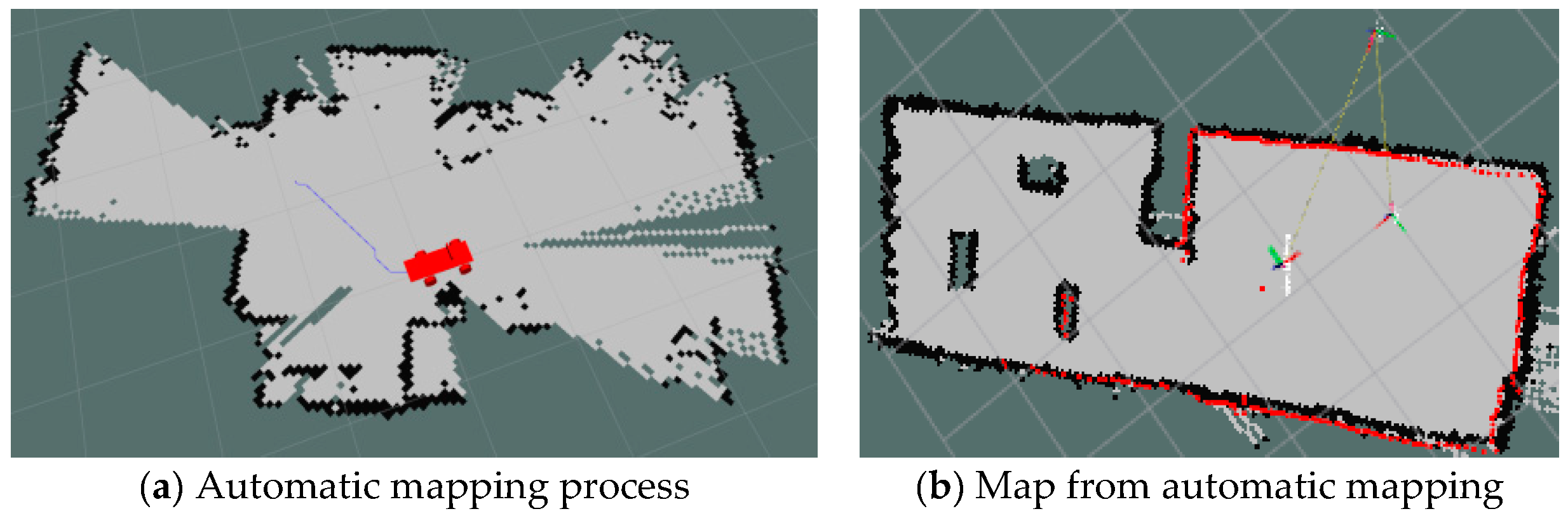
3.2. Simultaneously Localization and Mapping (SLAM) and Navigation System

As for SLAM, although it is based on a mature open source SLAM scheme, we revised it and proposed a novel automatic exploration scheme which can create maps automatically without the assistance from human interference. The basic principle of the automatic exploration is finding a frontier between known and unknown space in cost map and generating a desired trajectory to the destination. For example, when the car explores the indoor room, some frontiers of room will be displayed in the cost map, but other places in the room will not be displayed because these places are out of liDAR’s range or barricaded by other objects. Therefore, in order to explore unknown places, the car will firstly retrieve its previous trajectories until its starting place is found, compute the distance between starting place and current place, and move toward an unknown place far away from starting place. Secondly, the cost map is updated, and internal data is obtained if size of cost map has changed. To be exact, internal data is the increment grid map from last step to current step. Some grids are occupied by frontiers of object while other grids are not. Therefore, the direction of car in the next step is obtained by figuring out the number and direction of occupied and unoccupied grids. Thirdly, new trajectory to the unknown places is generated based on obtained internal data. Finally, new trajectory and the pose of the car are sent to the node of controller to generate the messages of steering. The steps of autonomous exploration in map generation of SLAM is shown in Figure 5.

The indoor map is conserved in the map server after being completely generated for navigation. Navigation module downloads the map from the map server and plan the global trajectory with the assistance of classical A* algorithm. Detail steps of SLAM and navigation are presented in the Figure 6.

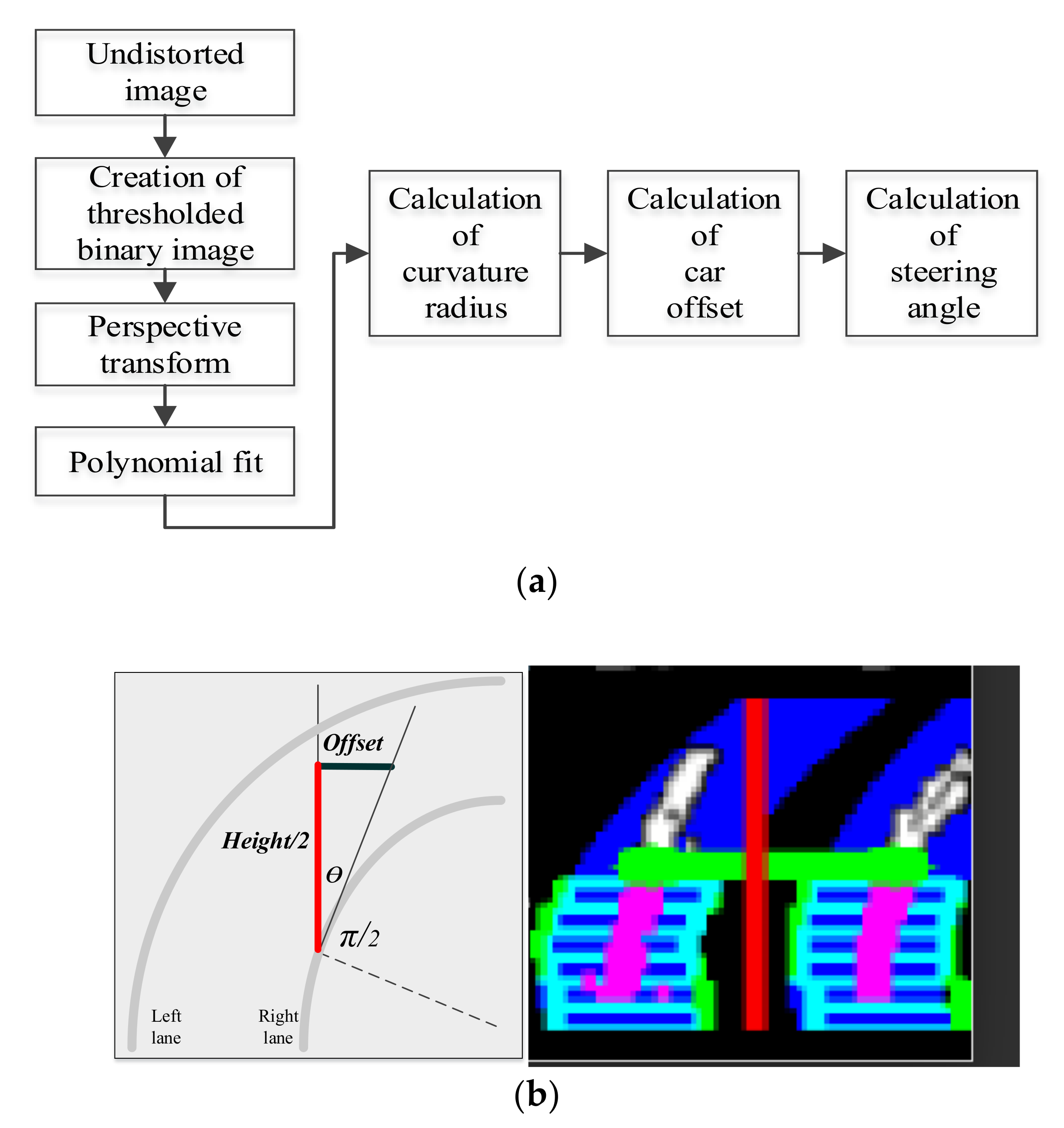
3.3. Lane Detection and Tracking

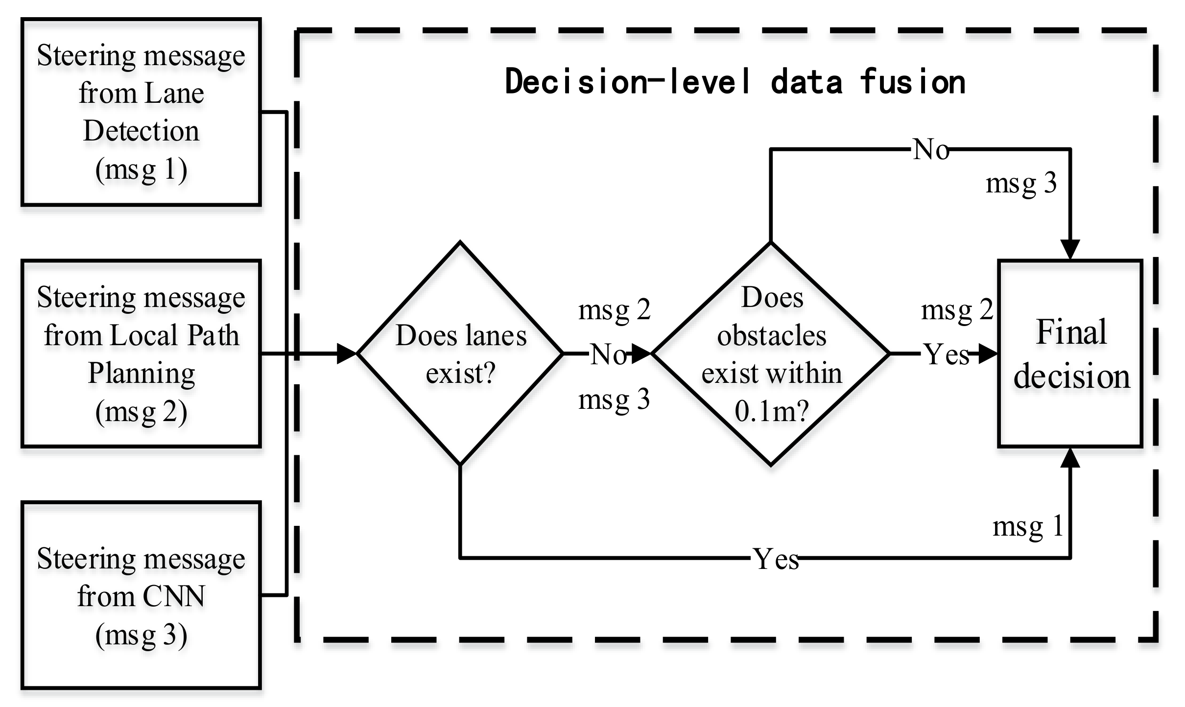
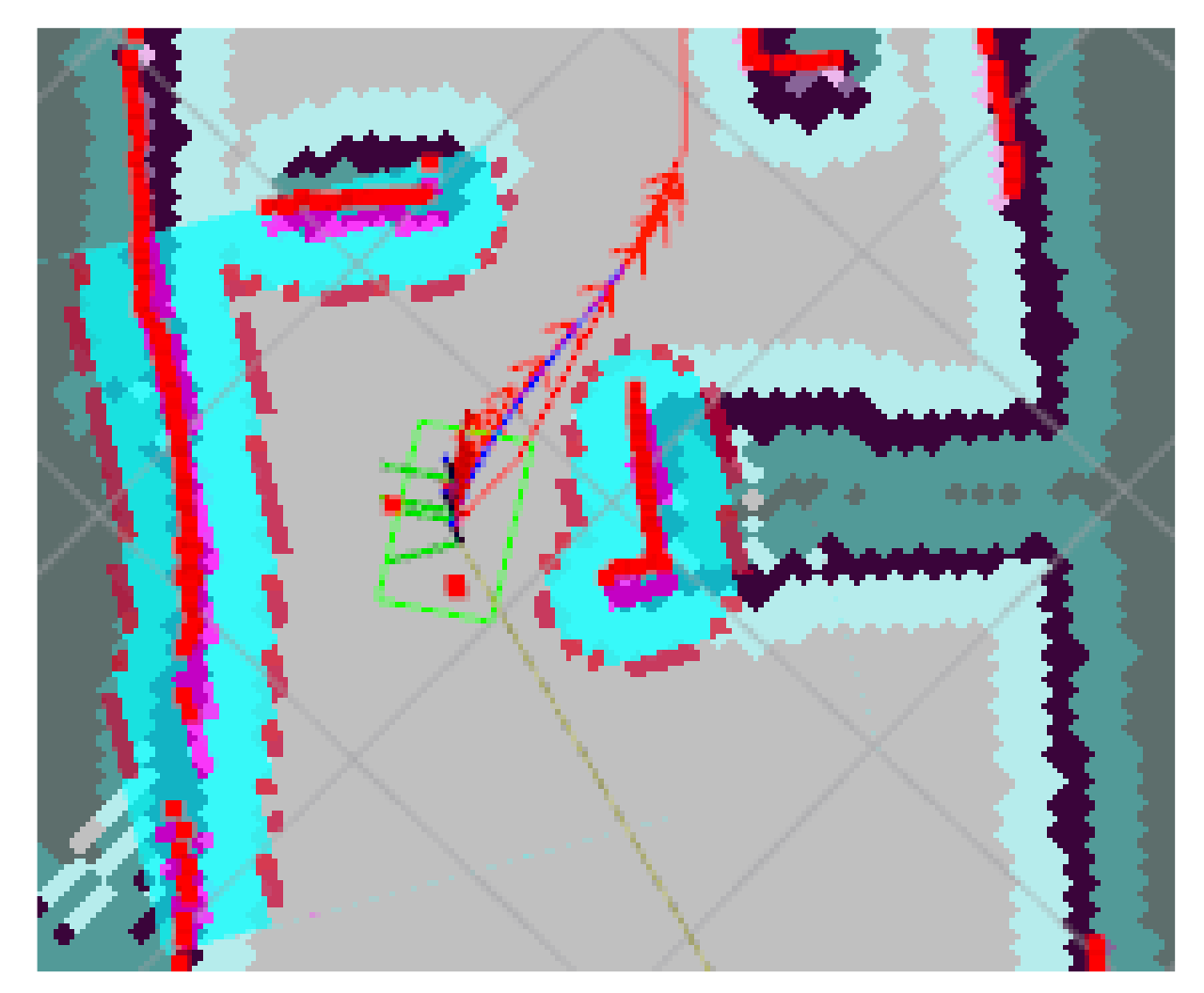
Earlier research in lane detection and tracking can be based on traditional image processing algorithms [27], while deep learning, and reinforcement learning are widely used in these years. This paper proposes an open computer vision (CV)-based method which meets real-time and costs lesser computing resource compared with the machine learning method.

Firstly, camera calibration is used to create undistorted images by using calibration matrices to revise the distortion of image. It is followed by using four filters with threshold, including absolute horizontal Sobel operator, magnitude of the gradient based on horizontal and vertical Sobel operator, direction of the gradient based on Sobel operator, and hue-lightness-saturation (HLS) transformation to create separate binary images and combine separate images together. Perspective transform is used to generate a “bird view” of binary images, while the bird-view image is also tailored in order to obtain an area which is most likely to have lane pixels. The bird-view images are split into two parts vertically in polynomial fit process, and then sliding windows which enclose 200 pixels are used to find the left and right lane. Once the pixel exists, sliding windows re-center their positions before second order polynomial to fit the window groups in left and right side. Left and right lanes are therefore generated. According to left and right lanes generated in previous step, Equation (3) is utilized to calculate the radius of curvature for each lane.

$$R=\frac{{\left[1+{\left(dx/dy\right)}^2\right]}^{\raisebox{1ex}{$3$}\!\left/ \!\raisebox{-1ex}{$2$}\right.}}{\left|d^{2}y/d{x}^2\right|}$$

(3)

In Equation (3), x and y represent pixel position in world space, and pixel space therefore must be converted into world space firstly using Equations (4) and (5).

$$x=x_{pixel}\cdot \alpha$$

(4)

$$y=y_{pixel}\cdot \beta$$

(5)

x_pixel and y_pixel represent the position of lane in pixel space, and x_pixel and y_pixel can be extracted directly from images. α and β represent the scale when the position of lane in pixel space is mapped to world space, and these values are 13/8300 and 70/115 respectively. The offset of car is calculated using Equation (6) under the assumption that the center of image is the center of car in real world.

$$offset=\frac{x_{image\_width}}{2}-\frac{(x_{left}+x_{right})}{2}$$

(6)

x_{image_width}, y_{image_height}, x_left, and x_right represent the width of undistorted image, the height of undistorted image, position of left lane, and position of right lane. Equation (7) is used to calculate the steering angle θ to generate steering messages for manipulating car.

$$\tan \theta =\frac{offset}{y_{image\_height}/2}$$

(7)

Steps of lane detection and tracking is presented in Figure 7a, and the process of computing steering angle in Equation (7) is illustrated in the Figure 7b.

3.4. Data Fusion

Decision-Level Data Fusion Design

A loose coupling method is adopted in the data fusion module. The loose coupling method integrates steering messages from different decision modules including steering messages from lane detection, messages from local path planning and messages from CNN to carry out decision-level data fusion. Firstly, top priority is given to steering messages from the module of lane detection and final decisions are generated directly once lanes exist, and steering messages are transmitted to the data fusion module. During this process, steering messages from lane detection will guide the car to drive along the lane until no lane is founded. Local obstacle avoidance function (local navigation) is completed using liDAR-based TEB method and deep learning method (CNN). The difference of these two methods is that TEB method is more suitable in emergent cases because liDAR-based method responses quicker than image-based method, but TEB method takes effect within 0.1~0.2 m while CNN method takes effect with a distance of two meters or much further. These two methods form a complementary, which means that emergent injuries or collisions can be avoided by using TEB method while the CNN method can be used to guild car to perform in a trained human-like way. Finally, integrated final steering messages are sent to hardware (Teensy3.6) to parse the steering messages to command that can be recognized and executed by hardware (motors and steering servos of car). Steps and priorities of steering messages are demonstrated in the Figure 8.

3.5. Auxiliary Modules

3.5.1. Data Recording

Data recording module is designed to record data including either raw data or processed data. Data comes from all sorts of sensors including the depth camera, the RGB camera, and liDAR. The data flow of the data recording module are presented in Figure 9.

Depth camera: depth camera can generate two sorts of images; RGB images and depth images respectively. RGB images are utilized in image recognition module (obstacle avoidance) because of its lower resolution, which is more suitable in deep learning case. Following this, RGB images are tailored, segregated and transformed into grayscale images. Additionally, real-time information that includes timestamp, value of steering angle and velocity value, are also attached as the label of processed images before being conserved. Depth images are also reserved for extended modules, like 3D SLAM and navigation.

RGB camera: unlike RGB images from the depth camera, images from RGB camera features high resolution due to the high frame rate of RGB camera. Additionally, the perspective of RGB camera for collecting images is also differentiated with depth camera. That means images from RGB camera contain lanes far away and also ensure the quality of images for a better land detection and tracking.

LiDAR: the map is generated using point cloud from liDAR in the SLAM module. The map is utilized for navigation, in which positions of car, surrounding obstacles and trajectories of car are also attached to previous maps and reserved simultaneously.

3.5.2. Message Parsing

Message parsing module bridges the software system and the hardware system. On the one hand, it receives final steering command and velocity command generated by software system. On the other hand, the commands are parsed and sent to hardware for actual decision making. In command parsing, ROS-based steering and speed messages are digital signals that are parsed to analog pulse signals. Analog signals can be recognized and executed by car (steering servos and motors) using approach of pulse-width modulation (PWM). To be exact, digital numbers ranged from 0.1 to 1.0 are utilized as the value of decision commands. Digital signals are mapped into the duty ratio of pulse width which can be recognized and executed by servos of hardware via message parsing module. By modulating the duty ratio according to the value of digital signals, desired trajectories of car can be generated at the same time.

Exponential smoothing is also utilized to smooth sharp changes of commands using Equation (8), in which V_init represents the initial value or real-time value of commands while V_change represents the sheer value (increment or decrease of commands). γ represents the intensity to smooth trajectories, and its value is 0.05.

$$V_{init}=V_{init}+\gamma \cdot (V_{change}-V_{init})$$

(8)

3.5.3. Proportion Integration Differentiation (PID)

Adaptive cruise control (ACC) is an adaption of the conventional cruise control system with additions of modulating throttle and applying braking, so as to vary the vehicle’s speed to follow the next closest vehicle [1]. In adaptive velocity control, a closed-loop PID control system is utilized in this module which receives wheels speed signals and steering angle signals from an encoder to regulate the speed of robotic car once dynamic or static obstacles are found. Steering messages, velocity messages and IMU messages are transmitted to SLAM and navigation module (odometer) where the position and pose of car are generated and sent to hardware (controller) to regulate the velocity of car under the control of PID.

4. Experiments and Conclusions

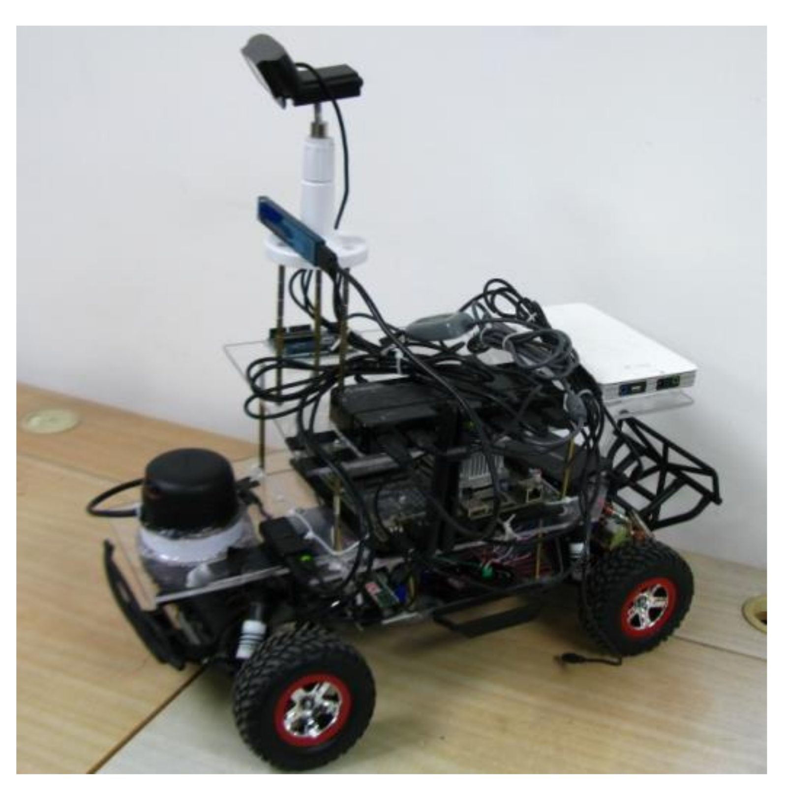
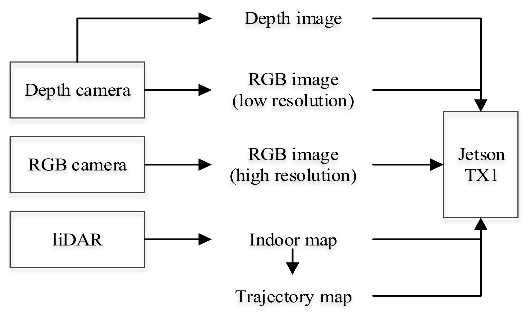
4.1. Hardware

Core sensors include Logitech C920 camera, Intel Realsense depth camera, RP-liDAR A2, 9 DoF IMU, Encoder, and Xbox360 stick controller. Digital-analog conversion (ROS messages parsing) is implemented in Teensy3.6. Traxxas car (1/10 F1 model) and is utilized as the chassis. All functional modules are integrated in nVidia Jetson TX1.

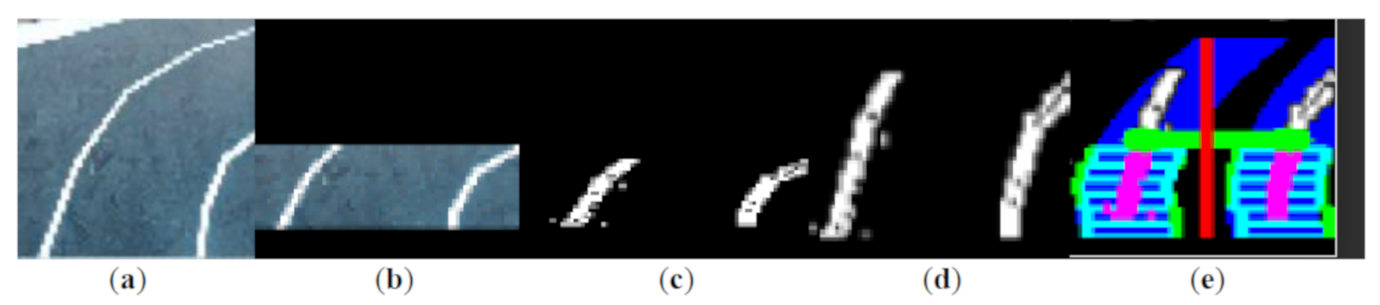
4.2. Result of Lane Detection and Tracking

In lane detection and tracking, the undistorted raw image is cropped (Figure 10b) after being captured from camera (Figure 10a) in order to reduce computing burden of image processing. Following this, the cropped image is converted into a binary image (Figure 10c), before being processed into “bird view” using perspective transform (Figure 10d). The last step is the polynomial fit which is the foundation of radius and offset calculation. In Figure 10e, a red line splits the image into two parts in the left and right sides. Light blue boxes represent sliding windows which are utilized to find lane pixels. Pink lines represent lane pixels found by sliding windows. Deep blue lines represent curves after the polynomial fit. A green line is indirectly used to calculate car offset.

4.3. Result of Intelligent Obstacle Avoidance

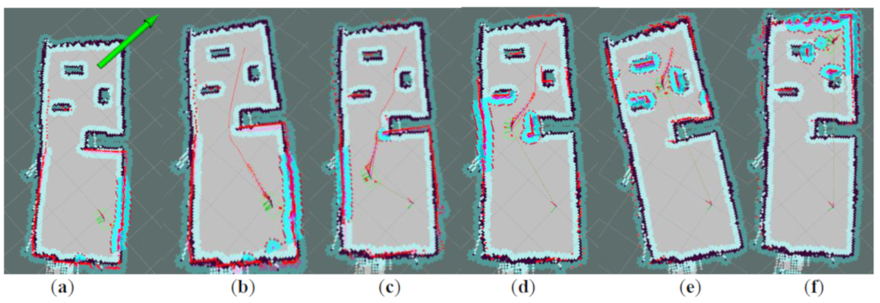
The Figure 11 represents the obstacle avoidance performance using TEB and the machine approach. The trajectory in the red color represents global path, while a deep blue line represents the local path which is optimized using a TEB and machine learning approach once obstacles are found in the short distance (0.1 m~0.2 m).

The recognition rate of obstacle based on CNN is presented in the Figure 12. Normally, obstacle avoidance approach based on CNN takes effect in a far distance and obstacle recognition rate can come to 97% averagely. The machine learning method based on CNN can guide car to behave in a trained human-like way. Note that CNN-based trajectories in obstacle avoidance and training details of a network can be found in the work of our team [28], in which we fuse the liDAR-based image processing approach with the deep learning approach in local obstacle avoidance or local motion planning. In the experiment of this paper, however, we fuse the TEB approach with the deep learning approach, and these approaches take effect in different ranges. That means the CNN-based approach can take effect in a longer distance, while the TEB-based approach takes effect in a shorter distance to avoid crashes in complex scenarios. In complex scenarios with more obstacles surrounded, these two methods are combined, and a robust trajectory is generated. The combination of these two approaches therefore enhance the robustness of robotic system in obstacle avoidance.

4.4. Result of SLAM

The experiment of SLAM was conducted in the indoor scenario (laboratory of university, Figure 2b), and results of SLAM are shown in the Figure 13. The Figure 13a represents a path that is found in the autonomous mapping process. The autonomous mapping process is expected to continue until the indoor space is completely explored. The Figure 13b represents an enclosed map after autonomous path finding process is terminated. The robotics therefore stops the process of exploration and the map is saved in robotics. Saved maps are expected to be updated frequently to keep the accuracy of the navigation.

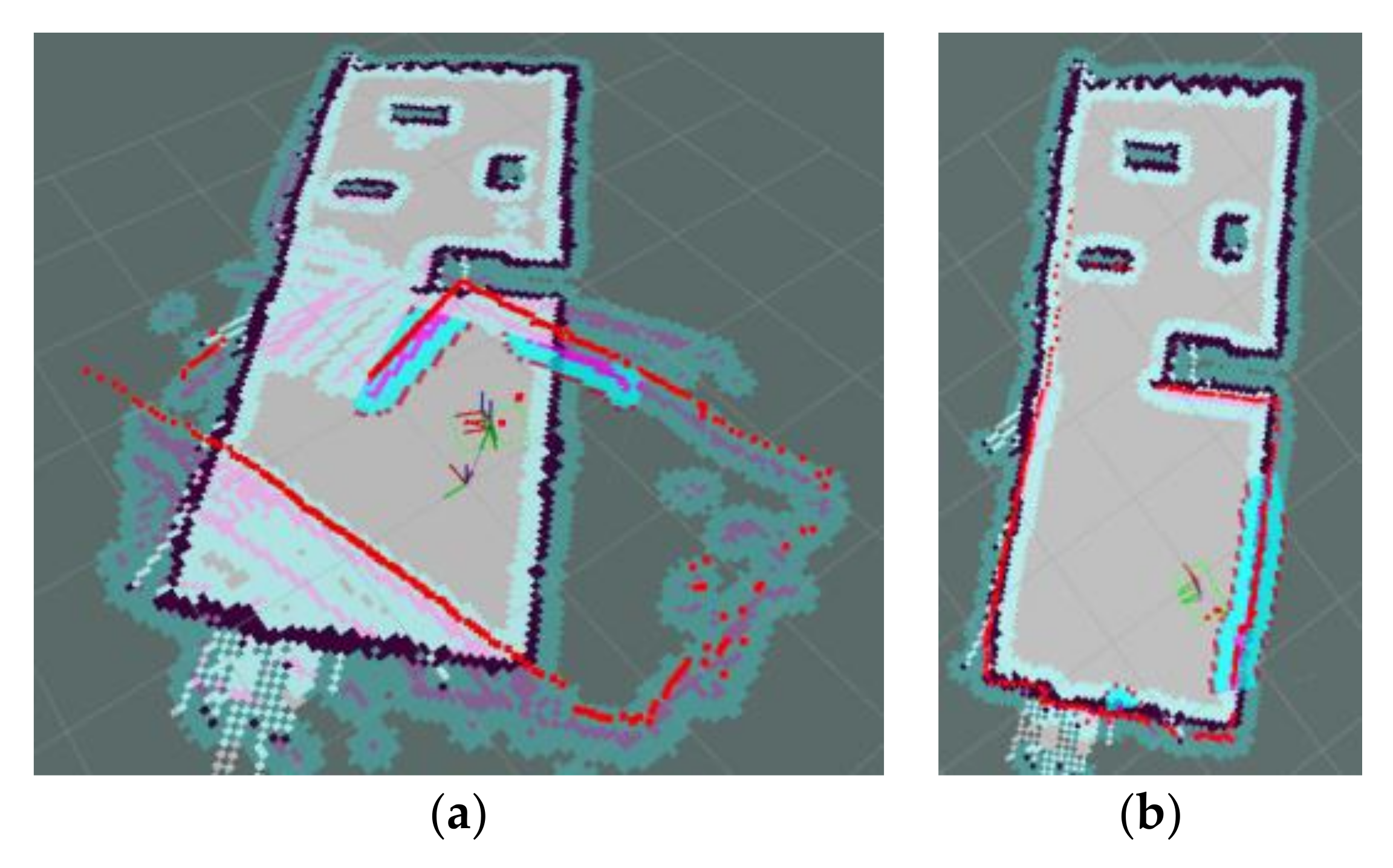
4.5. Result of Pose Estimation

The car can find the path autonomously (Figure 13a) until the overall enclosed map is fully constructed (Figure 13b). The enclosed map generated using SLAM will be saved and utilized in navigation. A 2D pose estimation function in RViz interface of ROS can be utilized to estimate the pose and position of car. Before the pose estimation, a point cloud from liDAR (red points) cannot match the map (Figure 14a), but after that the map can fit the liDAR data properly (Figure 14b).

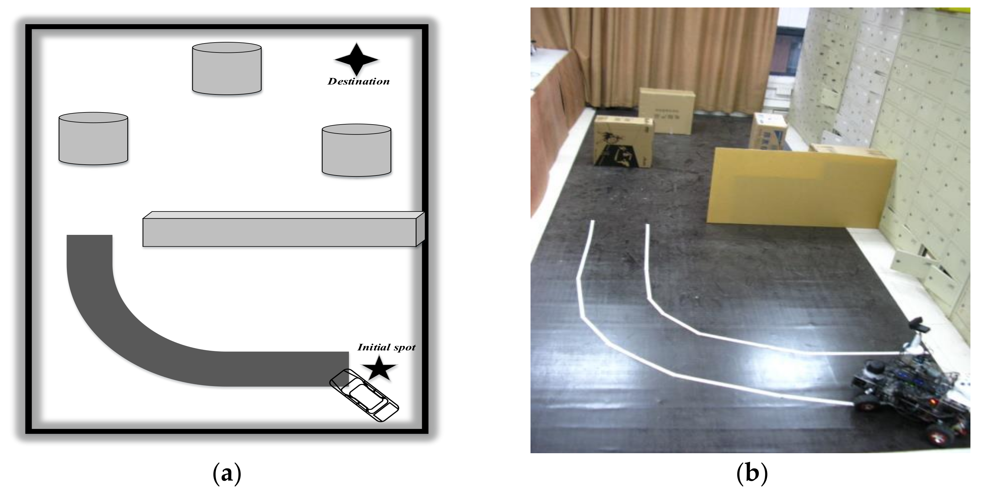
4.6. Result of Navigation

Before navigation, 2D navigation function in RViz interface in ROS should be utilized to set the destination and pose of car (Figure 15a). Following this, the car drives along the lane (Figure 15b~d)) (lane is not displayed in map directly) and after passing by the lane, the car walks abiding by the guidance of navigation (Figure 15e). Finally, the car reaches the destination successfully (Figure 15f).

5. Conclusions and Future Works

This paper demonstrates the design of architecture and implementation of functional modules in autonomous robotic car. Functional modules are composed by intelligent obstacle avoidance using CNN and TEB, SLAM, lane detection and tracking, data fusion, data recording, command parsing, velocity control, and hardware design.

This paper attaches much importance on proposing the architecture of autonomous car-like robot, features the fusion of all sorts of steering messages from different sensors, and fulfills all required functions successfully, instead of focusing on theoretical mathematical formulas or the optimization of specific algorithms.

In future works, priority will be given to enhancing the robustness and accuracy of functional modules by adding reinforcement learning in obstacle avoidance module, utilizing artificial neural network like deep learning approaches in data fusion, and applying 3D map in navigation.

References

1. Varghese, J.; Boone, R.G. Overview of autonomous vehicle sensors and systems. In Proceedings of the International Conference on Operations Excellence and Service Engineering, Orlando, FL, USA, 10–11 September 2015. [Google Scholar]
2. U.S. Department of Transportation Releases Policy on Automated Vehicle Development. N.p., 30 May 2013. Available online: https://mobility21.cmu.edu/u-s-department-of-transportation-releases-policy-on-auto- mated-vehicle-development (accessed on 20 March 2020).
3. Xu, P.; Dherbomez, G.; Hery, E.; Abidli, A.; Bonnifait, P. System architecture of a driverless electric car in the grand cooperative driving challenge. IEEE Intell. Transp. Syst. Mag. 2018, 10, 47–59. [Google Scholar] [CrossRef] [Green Version]
4. Wei, J.; Snider, J.M.; Kim, J.; Dolan, J.M.; Rajkumar, R.; Litkouhi, B. Towards a viable autonomous driving research platform. In Proceedings of the 2013 IEEE Intelligent Vehicles Symposium (IV), Gold Coast, Australia, 23–26 June 2013. [Google Scholar]
5. Cofield, R.G.; Gupta, R. Reactive trajectory planning and tracking for pedestrian-aware autonomous driving in urban environments. In Proceedings of the 2016 IEEE Intelligent Vehicles Symposium (IV), Gothenburg, Sweden, 19–22 June 2016; pp. 747–754. [Google Scholar]
6. Lima, D.A.D.; Pereira, G.A.S. Navigation of an autonomous car using vector fields and the dynamic window approach. J. Control Autom. Electr. Syst. 2013, 24, 106–116. [Google Scholar] [CrossRef]
7. Jo, K.; Kim, J.; Kim, D.; Jang, C.; Sunwoo, M. Development of autonomous car-part i: Distributed system architecture and development process. IEEE Trans. Ind. Electron. 2014, 61, 7131–7140. [Google Scholar] [CrossRef]
8. Jo, K.; Kim, J.; Kim, D.; Jang, C.; Sunwoo, M. Development of autonomous car-part II: A case study on the implementation of an autonomous driving system based on distributed architecture. IEEE Trans. Ind. Electron. 2015, 62, 5119–5132. [Google Scholar] [CrossRef]
9. Liu, L.; Wu, T.; Fang, Y.; Hu, T.; Song, J. A smart map representation for autonomous vehicle navigation. In Proceedings of the 12th International Conference on Fuzzy Systems and Knowledge Discovery (FSKD), Zhangjiajie, China, 15–17 August 2015; pp. 2308–2313. [Google Scholar]
10. Kunz, F.; Nuss, D.; Wiest, J.; Deusch, H.; Reuter, S.; Gritschneder, F.; Scheel, A.; Stübler, M.; Bach, M.; Hatzelmann, P. Autonomous driving at ULM university: A modular, robust, and sensor-independent fusion approach. In Proceedings of the 2015 IEEE Intelligent Vehicles Symposium (IV), Seoul, Korea, 28 June–1 July 2015; pp. 666–673. [Google Scholar]
11. Cardoso, V.; Oliveira, J.; Teixeira, T.; Badue, C.; Filipe, M.; Oliveira-Santos, T.; Veronese, L.; de Souza, A.F. A model-predictive motion planner for the IARA autonomous car. In Proceedings of the 2017 IEEE International Conference on Robotics and Automation (ICRA), Singapore, 29 May–3 June 2017; pp. 225–230. [Google Scholar]
12. Al-Harasis, R. Design and implementation of an autonomous UGV for the twenty second intelligent ground vehicle competition. In Proceedings of the International Conference on Software Engineering, Mobile Computing and Media Informatics (SEMCMI2015), Kuala Lumpur, Malaysia, 8–10 September 2015. [Google Scholar]
13. Ferreira, T.; Garcia, O.; Vaqueiro, J. Software Architecture for an Autonomous Car Simulation Using ROS, Morse and a QT Based Software for Control and Monitoring. In Proceedings of the XII Simpósio brasileiro de automação Inteligente, Uberlândia, MG, Brasil, 23–25 October 2015. [Google Scholar]
14. Memon, K.R.; Memon, S.; Memon, B.; Rafique, A.; Shah, A. Real time implementation of path planning algorithm with obstacle avoidance for autonomous vehicle. In Proceedings of the 3rd International Conference on Computing for Sustainable Global Development (INDIACom), New Delhi, India, 16–18 March 2016; pp. 2048–2053. [Google Scholar]
15. Parakkal, P.G.; Variyar, V.V.S. Gps based navigation system for autonomous car. In Proceedings of the 2017 International Conference on Advances in Computing, Communications and Informatics (ICACCI), Udupi, India, 13–16 September 2017; pp. 1888–1893. [Google Scholar]
16. Beiker, S. Implementation of an automated mobility-on-demand system. In Autonomous Driving; Maurer, M., Gerdes, J., Lenz, B., Winner, H., Eds.; Springer: Berlin/Heidelberg, Germany, 2016. [Google Scholar]
17. Shimchik, I.; Sagitov, A.; Afanasyev, I.; Matsuno, F.; Magid, E. Golf cart prototype development and navigation simulation using ros and gazebo. In Proceedings of the MATEC Web of Conferences, Punjab, India, 18 May 2016; Volume 75, p. 9005. [Google Scholar]
18. Evans-Thomson, S. Environmental Mapping and Software Architecture of an Autonomous SAE Electric Race Car. Ph.D. Thesis, The University of Western Australia, Perth, Australia, 2017. [Google Scholar]
19. Gupta, N.; Vijay, R.; Korupolu, P.V.N. Architecture of Autonomous Vehicle Simulation and Control Framework. In Proceedings of the 2015 Conference on Advances in Robotics, Goa, India, 2–4 July 2015; pp. 1–6. [Google Scholar]
20. Zhang, L.; Qin, Q. China’s new energy vehicle policies: Evolution, comparison and recommendation. Transp. Res. Part A Policy Pract. 2018, 110, 57–72. [Google Scholar] [CrossRef]
21. Tian, Y.; Pei, K.; Jana, S.; Ray, B. Deeptest: Automated testing of deep-neural-network-driven autonomous cars. arXiv, 2017; arXiv:1708.08559 [cs.SE]. [Google Scholar]
22. Du, X.X.; Marcelo, J.; Daniela, R. Car detection for autonomous vehicle: LIDAR and vision fusion approach through deep learning framework. In Proceedings of the 2017 IEEE/RSJ International Conference on Intelligent Robots and Systems (IROS), Vancouver, BC, Canada, 24–28 September 2017. [Google Scholar] [CrossRef]
23. Tobias, D.J. Cherry Autonomous Race Car. N.p., 6 Aug. 2016. Web. 29 May 2017. Available online: https://github.com/ DJTobias/-Cherry-Autonomous-Racecar (accessed on 24 March 2020).
24. Quinlan, S. Real-Time Modification of Collision-Free Paths; Technical Report; Stanford University: Stanford, CA, USA, 1995. [Google Scholar]
25. Fox, D.; Burgard, W.; Thrun, S. The dynamic window approach to collision avoidance. IEEE Robot. Autom. Mag. 1997, 4, 23–33. [Google Scholar] [CrossRef] [Green Version]
26. Smann, C.R.; Hoffmann, F.; Bertram, T. Kinodynamic trajectory optimization and control for car-like robots. In Proceedings of the 2017 IEEE/RSJ International Conference on Intelligent Robots and Systems (IROS), Vancouver, BC, Canada, 24–28 September 2017; pp. 5681–5686. [Google Scholar]
27. Pannu, G.S.; Ansari, M.D.; Gupta, P. Design and implementation of autonomous car using raspberry pi. Int. J. Comput. Appl. 2015, 113, 22–29. [Google Scholar]
28. Zhou, C.; Li, F.; Cao, W. Architecture Design and Implementation of Image Based Autonomous Car: Thunder-1. Multimedia Tools Appl. 2019, 78, 28557–28573. [Google Scholar] [CrossRef]
Figure 1. Intelligent car-like robot.
Robotics 09 00019 g001
Figure 2. (a) Represents the car in the abstract scenario, while (b) represents the car in real world.
Robotics 09 00019 g002
Figure 3. Overall control loop of robotic car. Functional modules in the control loop include the data collection (part 1), obstacle avoidance (part 3), lane detection and tracking (part 2), simultaneously localization and mapping (SLAM) and navigation (part 4), data fusion (part 5), and hardware and command execution (part 6). The arrival of a new position marks the end of one loop and the beginning of another loop.
Robotics 09 00019 g003
Figure 4. The framework of convolutional neural network (CNN) layers and data flow. Obstacle images are sent into CNN which is composed by three types of layers including CNN layer, flatten layer and full-connection layer. The probability of outputs and probability of expectation are therefore obtained. These two variants can be utilized to calculation the loss value. The weight of CNN is therefore updated using gradient approach.
Robotics 09 00019 g004
Figure 5. Steps of autonomous exploration in map generation of SLAM.
Robotics 09 00019 g005
Figure 6. Steps of SLAM and navigation. The module of SLAM and navigation can be divided into two parts, including map generation and saving, and navigation. On one hand, the robotic system generates maps and trajectories of robotics using data from sensors. The map and trajectory then is fused to another map that is saved in robotics. On the other hand, saved maps are utilized to generate the cost map that can be used to navigation based on the A* algorithm.
Robotics 09 00019 g006
Figure 7. (a) Represents steps of lane detection and tracking, and (b) represents the calculation of steering angles. The left image in (b) illustrates how to obtain the steering angle in the Equation (7) theoretically, while the right image in (b) represents the image from the experiment.
Robotics 09 00019 g007
Figure 8. Steps of data fusion and priorities of steering messages.
Robotics 09 00019 g008
Figure 9. Data flow of the data recording module.
Robotics 09 00019 g009
Figure 10. Lane detection and tracking. (a) Represents the raw image from the RGB camera. (b) Represents a selected part of raw image, and selected part is likely to have lane. (c) Represents the threshold binary image. (d) Represents a “bird view” after perspective transform. (e) Represents the image after polynomial fit. In (e), the read line represents the central line, and shallow blue boxes represent sliding windows, pinks lines represent lanes found by sliding windows, deep blue lines represent lines generated using polynomial fit, and green line is indirectly utilized to calculate the offset of car.
Robotics 09 00019 g010
Figure 11. Obstacle avoidance (local navigation) using the timed-elastic-band (TEB) approach. Red dots represent the obstacles found by liDAR (original data generated by liDAR). Shallow blue area represents the cost map. Green box represents the car and its pose. Red line represents the global planned path using A* approach. A short and deep blue line represents the local planned path using the combination of the liDAR-based TEB approach and machine learning methods. Arrows represent the direction of actual navigation. Planned paths generated by global planning using A* algorithm and local planning using TEB approach indicate that the path generated using TEB and machine learning approach is more short, smooth and robust than path generated using A* algorithm in the complex scenario.
Robotics 09 00019 g011
Figure 12. Obstacle recognition rate of trained CNN model. The experiment of obstacle recognition is conducted on the nVidia Jetson TX1 using Tensorflow-0.1. The X-axis represents the serial number of obstacle images in each batch, while the Y-axis represents the obstacle recognition rate. The recognition rate fluctuates and an average 97% is obtained in the experiment.
Robotics 09 00019 g012
Figure 13. The automatic mapping process of SLAM and the result of SLAM.
Robotics 09 00019 g013
Figure 14. Pose estimation. Shallow blue areas represent the cost map near the car. Grey area represents overall map. (a) Represents the map before pose estimation. In this map, we can notice that the source data from liDAR (point cloud) and the cost map cannot match the overall map generated using SLAM. (b) Represents the map after pose estimation. In this map, point cloud generated from liDAR and cost map match the SLAM map completely.
Robotics 09 00019 g014
Figure 15. Navigation using the map generated by SLAM. (a) Represents the destination and pose setting, and the rear of green arrow represents the destination, while the direction of arrow represents the pose of car. This process is completed by human manipulation. (b)~(e) Represent intermediate positions in navigation. We can notice that the car avoids the obstacles and arrives at the destination successfully. The car also detects and tracks lanes and successfully realizes this function, but lanes are not displayed in RViz (map). (f) Represents the arrival of destination. After that, the car will stop and wait for forthcoming command.
Robotics 09 00019 g015