1. Introduction
The multi-robot system is more robust, reliable, and precise than a single robot [
1,
2]. Thus, the multi-robot system takes place in many applications such as reconnaissance and security patrol operations and search and rescue missions [
3]. One of the main problems in the multi-robot system is the formation control. The formation of the multi-robot system is a cooperative behavior of the interacting mobile robots sharing one goal [
4]. Therefore, lots of research studies have been presented in this field. Some of these researchers depend on a central controller such as [
5,
6,
7]. However, these methods are very prone to failure. Thus, they are not suitable for the formation problem [
8]. Therefore, decentralized formation control methods are suggested such as the Potential Field Method (PFM) [
9]. The PFM was first introduced for robot navigation by Khatib in 1986 [
10]. The PFM gains its popularity due to its simple structure and it reduces the information used in the calculations. Thus, the PFM is considered a suitable technique for navigation in the real-time application [
11].
However, the PFM suffers from some limitations such as oscillation near obstacles or at narrow passages. Also, it suffers from the local minima problem (LMP) where the obstacle is placed between the robot and its target and they are placed on the same line [
11,
12]. So, many solutions were presented to solve the PFM problems.
In this article, we propose a fuzzy tuning method for PF parameters to solve its limitations. The tuning method online tunes the PF parameters according to various situations the robots may face. Then, we apply the modified PFM to a group of TurlteBot3 robots. So, we conduct a set of real-time experiments to verify the applicability of the modified PFM and verify its ability to solve the traditional PFM limitations.
In the following section, we begin with a brief review of the related research. Next, we present the modified PFM and the proposed FIS tuning method in
Section 3. In
Section 4, we demonstrate the implementation of the modified PFM with the tuned parameters and the system’s hardware used in the verification. Then,
Section 5 shows a set of real-time experiments on Turtlebot3 robots and the experimental results followed by the discussion in
Section 6. Finally, a conclusion for our work is presented in
Section 7.
2. Review on the Related Research
The literature is rich in many solutions for PFM limitations. For example, Li et al. [
13] proposed an evolutionary Artificial Potential Fields (APF) approach for path planning. Their simulation result showed that the evolutionary method is effective for solving the local minimum problem, but it did not solve other problems. In addition, Wang et al. [
14] proposed a formation control method where the potential functions were used between agent–agent and between agent–obstacle. Their method helped avoid local minima. Simulations showed the rationality of this control method but they did not overcome other problems. In addition, Zhang et al. [
15] constructed a dynamic APF based on the local information to solve the problem of the traditional PFM where collisions among robots were avoided by the repulsive PF among them. They proposed a solution for the global minimum point by adjusting the movement direction of the robot within an escaping area. Simulation results validated the effectiveness and practicability of the proposed formation control algorithm based on the proposed dynamic APF.
Bennet and McInnes [
16] proposed a pattern formation for a multi-robot system using a bifurcating Potential Field (PF) control algorithm. They showed that changing free parameters could achieve various patterns. Simulation results proved the stability of the system and ensured that desired multi-robot behaviors always happen. In addition, Bennet et al. [
17] developed a bounded bifurcating PF guidance algorithm for the formation of unmanned aerial vehicles (UAVs). They proved that the formation of UAVs can be controlled by the bifurcating PF approach where the verifiable autonomous patterns were achieved with a simple parameter to switch between patterns. Simulations showed that the three-dimensional formation flight for a swarm of UAVs could be achieved. Ranjbar-Sahraei et al. [
18] presented a decentralized adaptive control scheme for multi-agent formation control based on an integration of APF with robust control techniques. They considered fully actuated mobile agents with partially unknown models, where the unknown system dynamics were approximated by an adaptive FIS. The proposed controller was robust to input nonlinearity, model uncertainties, and external disturbances. Simulation results illustrated the effective attenuation of approximation errors and external disturbances. Moreover, experimental results confirmed the validity of the presented approach and verified the applicability of the scheme for a swarm of six real holonomic robots.
Furthermore, Kowdiki et al. [
19] proposed a formation control of a group of mobile robots using the APF where the leader robot of the group determined its navigation path via the PFM, avoided the collisions with the obstacles, and followed an optimal path to reach its goal position. The other robots in the group followed the leader, adapting their formation by controlling the desired separation distance and the bearing angle. So, the formation could be recovered after being lost due to passage through a narrow path. Therefore, the formation control scheme resulted in a robust and adaptive formation control for a group of mobile robots. The effectiveness of the proposed formation control was verified by simulation. Besides, Dang and Horn [
20] presented an APF-based approach to control robots to quickly find their swarm and avoid obstacles while tracking a moving target. The APF between each free robot and the virtual attractive point of the swarm led them to the swarm. The connections between member robots with their neighbors were controlled by the artificial force to avoid collisions and keep the formation among them. Simulations verified the effectiveness of the proposed approach. They also suggested in [
21] an approach based on the PFM and a state feedback controller for the formation control of a swarm of UAVs tracking a moving target in a dynamic environment. The effectiveness of their proposed approach was verified in simulations.
Moreover, Furferi et al. [
22] presented a decentralized approach based on Artificial Neural Networks (ANNs) for the cooperative mobile manipulation of underwater mobile robots. This approach used the PFM for a multi-layer control structure to manage the coordination, the guidance, and the navigation of underwater mobile robots. They simulated the transportation of an object that moved along a desired trajectory in an unknown environment by four underwater mobile robots. Then, they optimized the simulation results by ANNs for the tuning of PF parameters. In addition, Elkilany et al. [
23] proposed an adaptive formation control algorithm based on the PFM for robot swarm. An ANN was employed to improve the performance of the PFM. The ANN optimized the synaptic weights in each layer and then updated the PF parameters. MATLAB simulation verified the modified PFM. Yin et al. [
24] suggested a formation tracking control for multiple UAVs flying through a constrained space. The proposed technique guaranteed to maintain a given formation among UAVs while avoiding collisions. Simulation results illustrated the validity of proposed formation control.
In addition, Han et al. [
25] proposed a control algorithm that combines the target allocation algorithm with an obstacle avoidance algorithm to prevent the multi-robots forming an arbitrary formation. They expressed the distance between the robots and target points by distance information matrix to ensure that each robot finds its target point. The obstacle avoidance was achieved by improving the APF integrated with obstacle avoidance. Simulation results showed that the proposed method is feasible and effective. Besides, Elkilany et al. [
26] presented a formation control algorithm based on the PFM and Fuzzy Inference System (FIS). They added an interaction potential force to maintain formation beside the attractive and repulsive potential forces. Moreover, they used an FIS to adapt to the change of the relative distances among robots and other entities in the environment. They tested the scalability and reliability of their proposed formation control algorithm by simulations.
These contributions solved one or two of the PFM problems, but they did not solve all of them. In addition, most of these solutions were tested in a simulated environment, not in real-time, ignoring real-time experiment problems and challenges. Thus, we aim to propose a solution to overcome the limitations of the PFM and to use real-time experiments to verify our method.
3. The Modified Potential Field Method
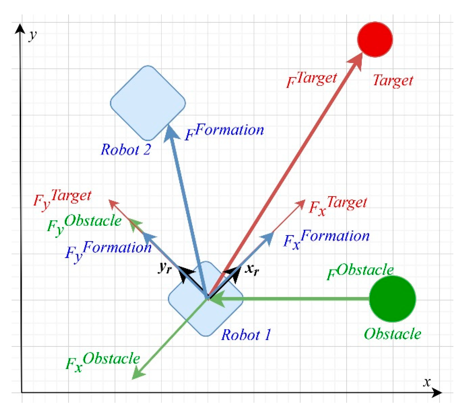
In the formation problem, each robot should track a moving target, avoid obstacles, and keep a fixed distance between the robot and other robots in the environment. As illustrated in
Figure 1, each robot is affected by three forces: the target tracking force
, the obstacle avoiding force
, and the formation maintaining force
. In this case,
and
are in the same direction of the robot movement, while
is in the opposite direction.
The applied potential forces depend only on the distances among the three objects in the environment: the distance between a robot and a target, a robot and the detected obstacles, and a robot and its neighboring robots. In the next subsections, we introduce the three applied forces in detail, followed by the proposed tuning method via FIS.
3.1. The Applied Potential Forces
The target tracking force is an attractive force that pulls the robot to its target. The target tracking force
for
is defined as:
where
is the instantaneous position of
and
is the instantaneous position of the tracked target according to the environment global frame.
is the distance between
and the target, and
is the target tracking range.
The obstacle avoiding force
is a repulsive force that pushes
away from
. The obstacle avoiding force depends on the robot–obstacle distance
. The obstacle-avoiding force for
avoids
is given as:
where
is the obstacle detecting range and
is the unit vector from
to
,
where
is the instantaneous position of
according to the environment global frame.
The third force is the formation-maintaining force, which is an attractive force if the robot is far from its neighbor and a repulsive force if the robots are very close to each other. This force depends on the distance
between
and its neighbor
. The formation-maintaining force
between a
and its neighbor
, where
, is given by:
where
is the formation range. Thus, the control input controlling the motion of
is the summation of the three forces as is given in the following equation:
where
is the number of robots and
is the number of obstacles detected by
,
, and
are the target tracking gain, obstacle avoiding gain, and formation maintaining gain, correspondingly. They are also known as the PF parameters. These gains/parameters can change the magnitude of each applied force according to its contribution to the robot’s movement. In the next subsection, we propose an FIS to tune these gains to adapt to the changes in the environment around the robots.
3.2. The Proposed Fuzzy Inference System
Three potential forces are controlling each robot. Still, the magnitude of each force should vary according to the situation the robot faces. Thus, the potential forces are weighted by the PF gains/parameters
,
, and
. To make the resultant force adaptively change according to the various situations, we tune the PF gains, so the magnitude of each force is tuned to successfully escape from the embarrassing situation the robot is facing. Therefore, we propose a Mamdani-FIS [
27] to adaptively tune the PF parameters according to the robot’s status in the environment. FIS is considered an intelligent control system and it deals with the system’s uncertainty and nonlinearity [
28,
29].
The proposed FIS captures each robot’s status and produces the tuned PF parameters. The status of each robot is defined by the distances among the robot and other entities in the environment. The number of robot-to-obstacle distances depends on the number of obstacles around the robot during the real-time experiment. As we use the LiDAR sensor, which gives a 360 reading per time (which is a 2D laser scanner that senses 360° with an angular resolution of 1°), the maximum number of obstacles around a robot is 360 obstacles. Thus, the maximum number of robot-to-obstacle distances is 360 and the minimum number is 0 where no obstacles around the robot are detected. Thus, we depend only on the distance between a robot and the nearest detected obstacle . The number of robot-to-robot distances depends on the number of the robots and subsequently the number of neighbors for each robot. Thus, the maximum number of neighbors is . In addition, as the minimum number of robots in a group is 3, so the minimum number of neighbors is 2. Therefore, in our proposed FIS model, we use only four distances: robot-to-target (, robot-to-nearest obstacle (, robot-to-the first nearest neighbor , and robot-to-second nearest neighbor .
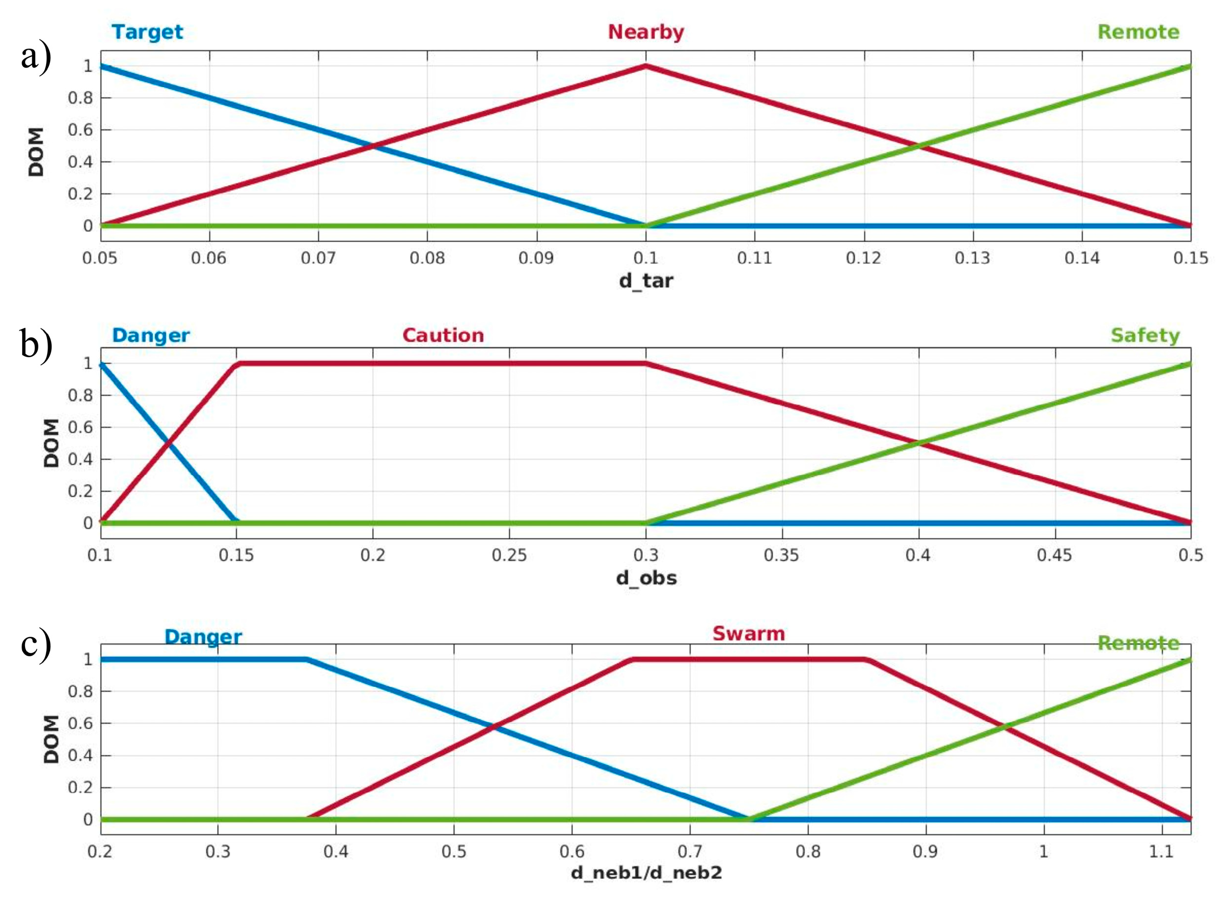
3.2.1. Fuzzy Inputs
The first step is to fuzzify the FIS inputs. In our proposed FIS, we have four inputs. The first input is the robot-to-target distances
. It is divided into three regions. The first is the “Target”, where the robot is close to its target as determined by
. The second region is "Nearby”, where the robot is not close to the target. The third region is “Remote”, where the robot is very far from its target. The second input is the robot-to-nearest obstacle distance
. This distance is divided into three regions from 0.1 mm to 0.5 mm according to the scan region, accuracy, and precision of the used LiDAR sensor. The first region is “Safety”, where the obstacle is not close to the robot or not detected by the LiDAR sensor. The second region is “Caution”, where the robot can detect a close obstacle. The third region is “Danger”, the critical region, where the obstacle is very close to the robot. Similarly, the third and fourth inputs are also divided into three regions. The first one is “Remote”, where the robots are far from each neighbor. The second one is “Swarm”, where the distances among robots are within the required range
. The third one is “Danger”, where the robots are so close so that they may collide.
Figure 2 shows the fuzzification, the universe of discourse, and the corresponding degree of membership for inputs.
3.2.2. Fuzzy Outputs
Our proposed FIS has three outputs. The first output is the target gain
, which is divided into four fuzzy sets: “S”, Small; “M”, Medium; “L”, Large; and “V.L”, Very Large. The second and third outputs
and
are divided into three membership functions: “S”, Small; “M”, Medium; and “L”, Large. The universe of discourse of the three outputs is normalized (between 0 and 1).
Figure 3 shows the fuzzification, the universe of discourse, and the corresponding degree of membership for fuzzy outputs.
3.2.3. Fuzzy Rule Base
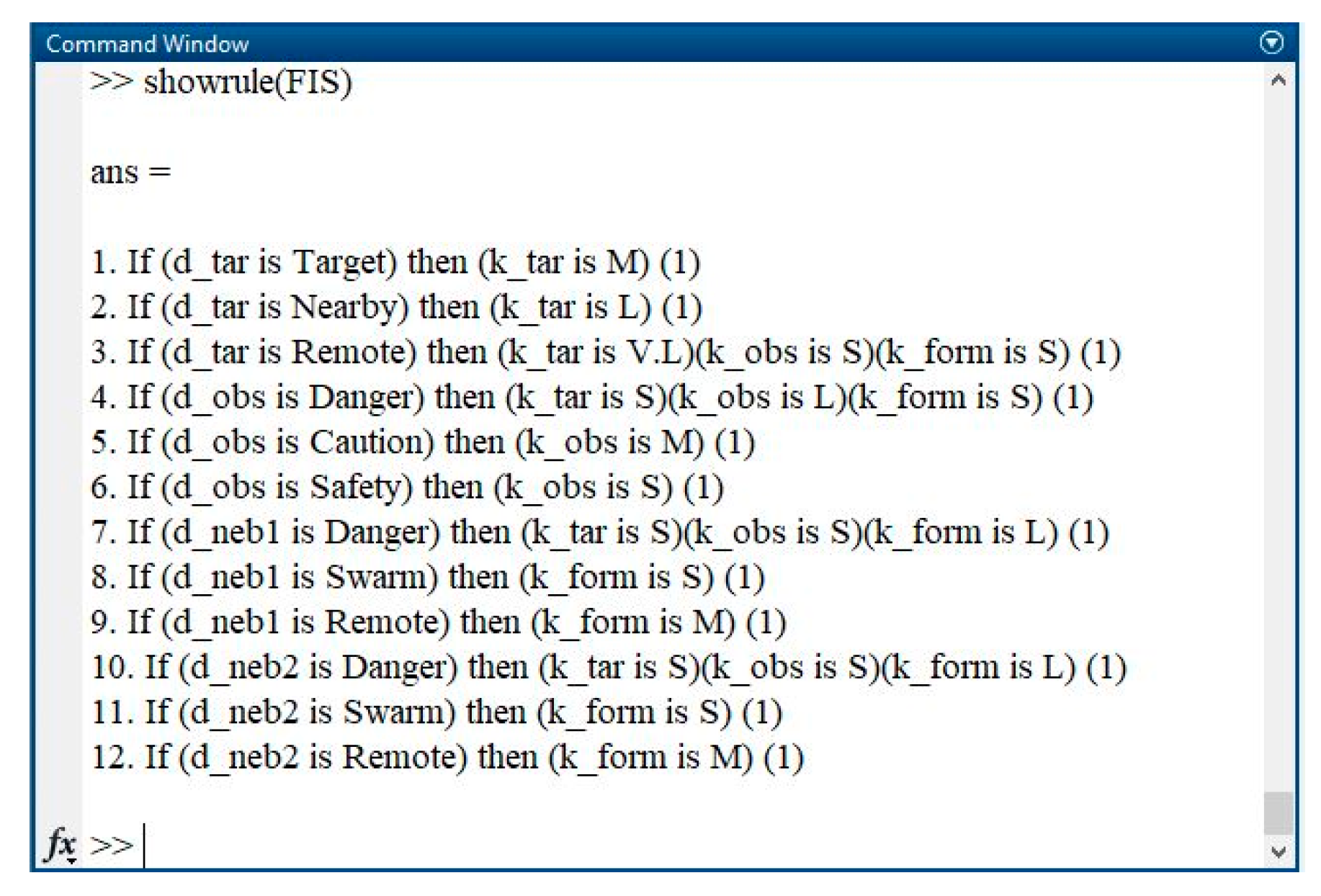
After studying the relationship between distances, forces, and the gains, the fuzzy rules are proposed.
Figure 4 displays the fuzzy rules as implemented in MATLAB. As is illustrated in the figure, the fuzzy rule base contains only 12 rules regardless of the number of robots or the number of detected obstacles. This makes our proposed FIS scalable for any number of robots.
4. System Implementation and Architecture
To test the modified PFM, we set up a system of physical robots and apply several real-time experiments. Three Turtlebot3 robots equipped with some sensors and actuators are employed. Then, we implement the modified PFM with FIS tuning and other functions to control the robots. In the following, we present a detailed description of the hardware and the software in our system.
4.1. System Hardware
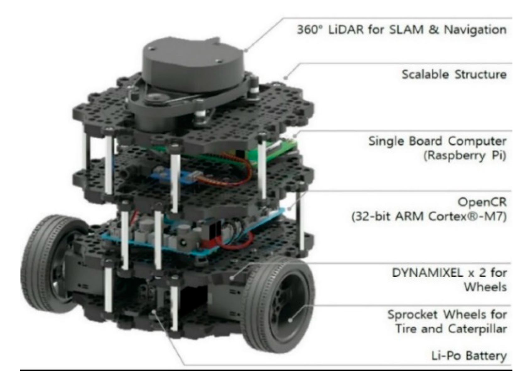
Three TurtleBot3 Burger Model robots are used to form a group of identical robots. The TurtleBot3 robot [
30] is a modular mobile robot provided with a
360° laser distance sensor LDS-01 (LiDAR). The LiDAR is a 2D laser scanner that senses 360° with an angular resolution of 1° and collects data about the environment around the robot with scan rate equals to 300 ± 10 rpm and a sampling rate equal to 1.8 kHz [
31]. Its detection distance is 120 mm to 3500 mm with a distance accuracy ± 15 mm, distance precision ± 10 mm for 120 mm to 499 mm, and distance accuracy ± 5% and distance precision ± 3.5% for 500 mm to 3500 mm.
In addition, each robot has two boards. First, the OpenCR board [
32] is a low-level board for controlling servo motors. It is equipped with an Inertial Measurement Unit (IMU) sensor reporting the orientations of the robot. Second, the Raspberry Pi board [
33] is used for high-level programming. This kit is the latest revision of the third generation single-board computer. The speed of its CPU is 1.4 GHz. In addition, Model B+ has a dual-band wireless antenna, supporting both 2.4 GHz and 5 GHz 802.11 b/g/n/ac Wi-Fi. Therefore, communication among robots can be held through the Wireless Local Area Network (WLAN). Furthermore, the robot is equipped with the DYNAMIXEL XL430-W250-T smart actuator system [
34]. The DYNAMIXEL is a high-performance actuator integrated with DC Motor, Reduction Gear head, Controller, Driver, and Network. It has a contact-less absolute encoder as a position sensor.
Figure 5 shows the main components of the TurtleBot3 Burger Model robot, as presented in [
34].
4.2. System Software
To control the robots, we implement the PFM equations in MATLAB software. In addition, we construct the proposed FIS using the fuzzy toolbox in MATLAB. Other functions are also created to control sending and receiving data to or from the robots.
Figure 6 displays the flowchart of our proposed formation control, which runs independently on each robot. After initialization, the status of the robot is recorded by receiving data from the robot’s sensors. The robot orientation is detected by the IMU sensor, and the obstacles detected around the robot are sensed by LiDAR. The robot calculates its position from the position sensor (encoder) and broadcasts its position to other robots. It also listens to other robots to receive their current positions. To accelerate the performance of MATLAB, we use Parallel Computing Toolbox. However, in this case, there is no shared memory, so that each robot should broadcast some data about itself via a WLAN.
After exchanging these data, the distances between every two objects are calculated to call the proposed FIS. FIS receives the distances
,
,
, and
and calculates the PF parameters
,
, and
by calling the proposed rule base. Then, the PFM equations are applied to compute the control input
from Equation (4). Then, from
, the linear and angula/4r velocity
and
are computed and are sent to the robot to move. These steps are repeated until the predefined maximum execution time
. Time is measured by the ROS server (which is a platform allowing data sending and receiving and control [
35]).
5. Experiments and Results
In this section, we test the applicability of the modified PFM with the tuned parameters using FIS. We aim to illustrate how the FIS tuning of the PF parameters solves some of the limitations of the traditional PFM such as oscillating near narrow passages or near closely placed obstacles. Moreover, the modified PFM should help the robots achieve their main three tasks, avoid obstacles, track a given trajectory, and maintain a formation among robots.
Thus, we conduct a set of real-time experiments for each PF limitation and set two criteria to judge the performance of the robots. We examine the ability of the robots to pass through a narrow passage, pass through closely placed obstacles, and escape from the LMP.
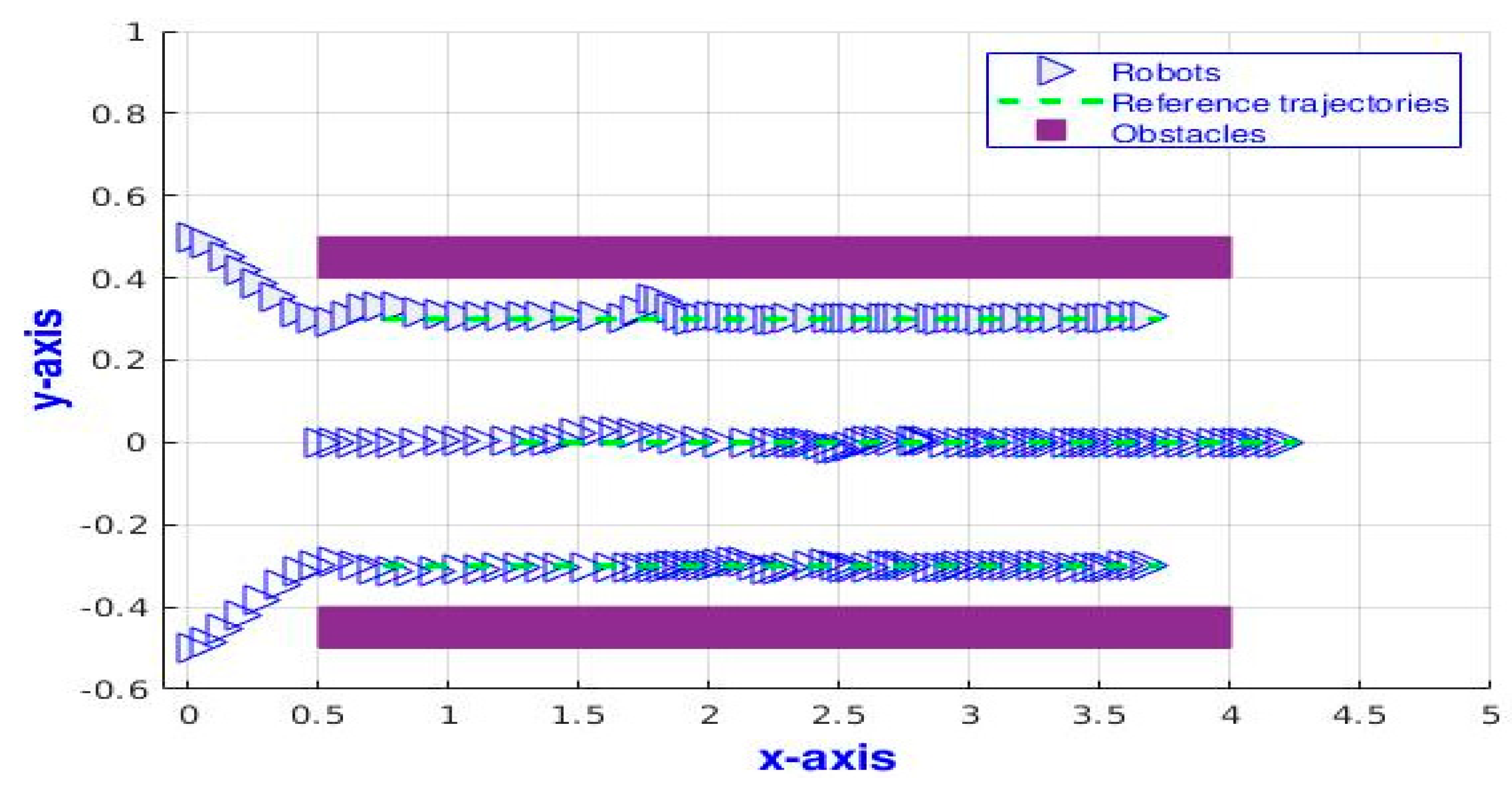
5.1. Passing Through A Narrow Passage
In this test, we set up a narrow passage for the three TurtleBot3 robots and record the robots’ response. The time response is displayed in
Figure 7, which shows that the three robots are passing through the narrow passage in the x-y plan. It also shows that the robots do not oscillate around the obstacles and succeed in passing through the passage. Besides, the robots manage to track the given trajectory with high accuracy, as shown in
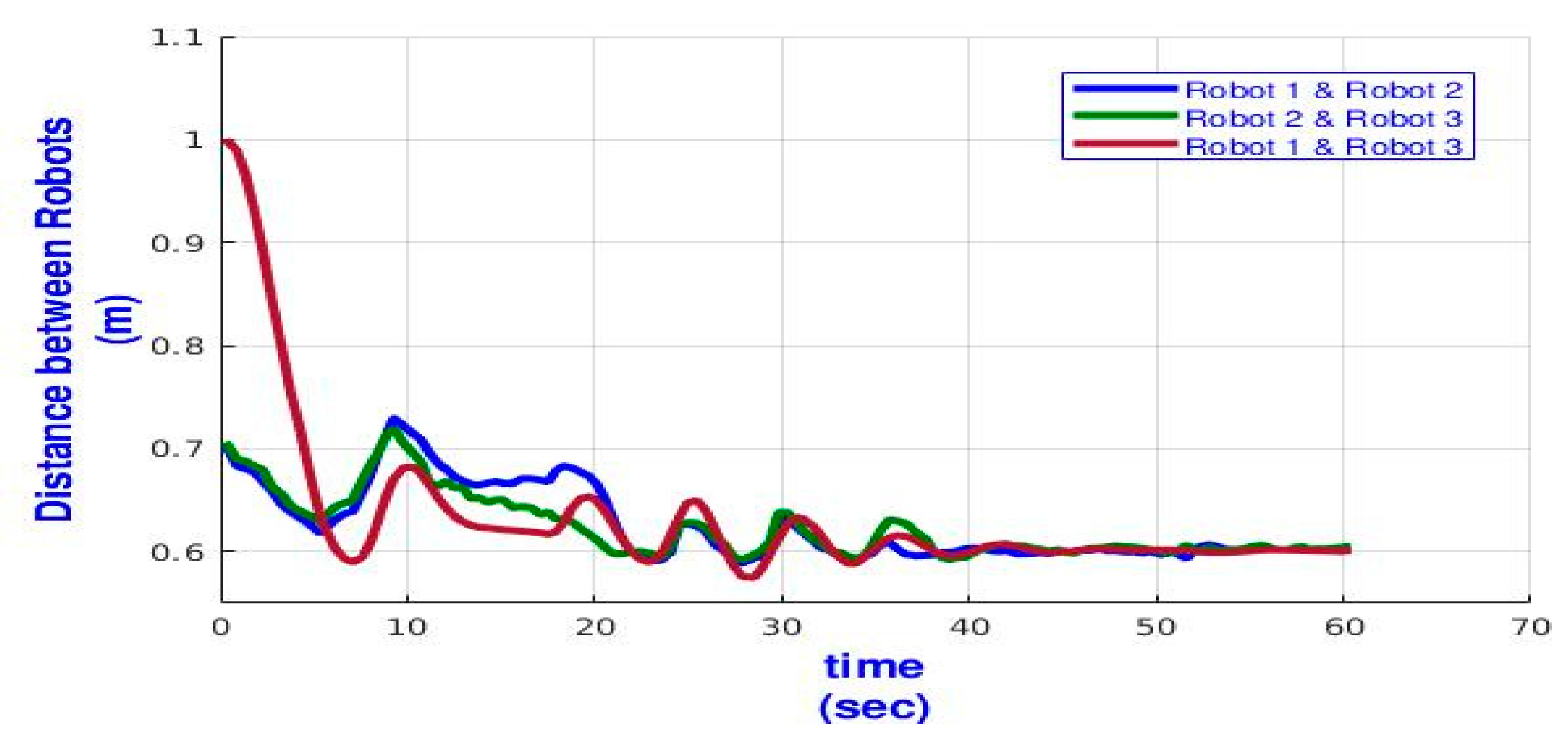
Figure 8. Moreover, the robots maintain a fixed distance among themselves while tracking the trajectory, as shown in
Figure 9. Where the distances between each two robots are initially very large, then, they oscillate around the formation range
. Finally, they steady state at the required value.
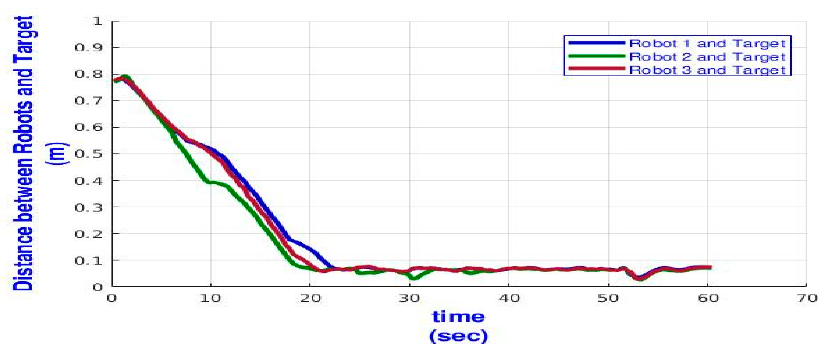
We repeat this test for five independent runs to extract some statistical data.
Table 1 presents the maximum and average of the tracking error
, which indicates the robot’s success in the tracking task. A low value of the tracking error
means a high tracking accuracy. From the data, we find that the maximum
in five sequential independent runs for the three robots ranges from a minimum value equal to 0.6822 to 0.7043 m, and the average of
ranges from 0.0738 to 0.1272 m. In addition, we find that during the run time, the accuracy of tracking reaches 97.9%, 98.3%, and 97.8% for Robot 1 (R1), Robot 2 (R2), and Robot 3 (R3), respectively. Thus, the overall tracking accuracy for all the robots is approximately 98%.
For formation accuracy, we calculate the formation error, which shows how the distance between two robots is far from the required distance or the formation range.
Table 2 shows the minimum, maximum, and average values of the formation error
. As is shown, the maximum value of the minimum
is 0.0487 m, where the maximum
value of the maximum is 0.4 m, and the minimum value reaches 0.11 m. In addition, the average
ranges from 0.0132 to 0.0451 m. Thus, the formation accuracy reaches 99.5%, 99.4%, and 99.2% for R1, R2, and R3, respectively. Thus, the overall formation accuracy for all the robots is approximately 99.4%.
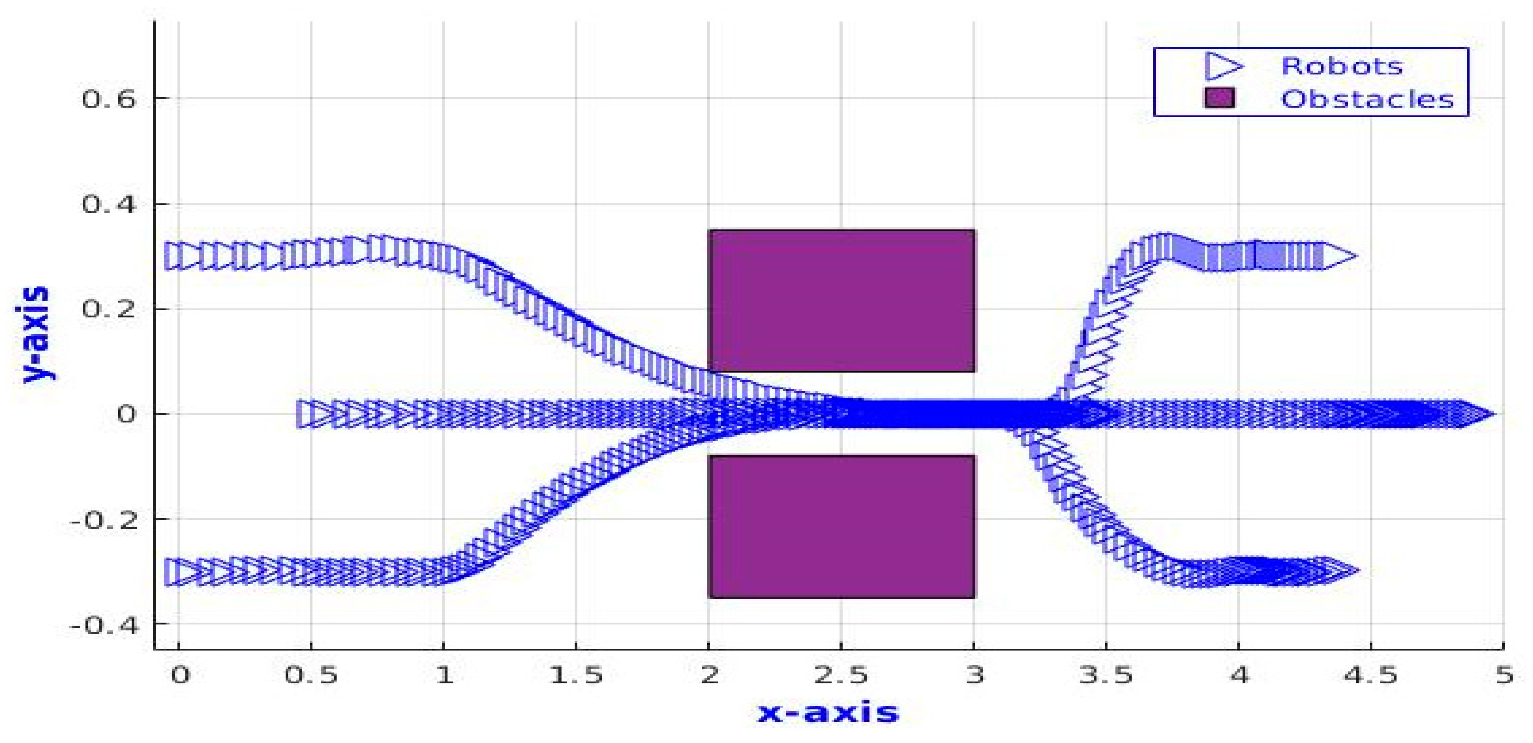
5.2. Passing between Two Closely Placed Obstacles
Another challenge of the traditional PFM is to pass between two closely placed obstacles. The robot may oscillate near obstacles and not pass these obstacles. Thus, in this test, we verify the ability of the TurtleBot3 robots to pass through closely placed obstacles. The robots give a higher priority to passing the obstacles than they give to formation. The time response of the three robots is illustrated in
Figure 10. The robots break the formation, follow each other, pass the obstacles, and then return to their formation again.
Figure 11 also shows the distances between every two TurtleBot3 robots where the distances start from the required distance or the formation range
. Then, the distances reduce to reach 0.2 m while the robots pass the two closely placed obstacles. Finally, the distances increase again to reach the required formation distance.
5.3. Escaping from the LMP
Traditional PFM also suffers from the LMP where an obstacle is placed between the robot and its target. In this situation, the target tracking force that pulls the robot to the target is equal to the obstacle avoiding force that pushes the robot away. Thus, the robot does not move or oscillate. In our case, each robot is controlled by three types of forces. The LMP occurs when the summation of the applied forces equals zero, preventing the robot from moving. Thus, in this test, we examine the ability of the modified PFM to escape from the LMP.
Figure 12 shows the real TurtleBot3 robots avoiding various obstacles during the experiments. In the first experiment, one obstacle is placed on the path of the central gravity of the three TurtleBot3 robots. We observe that the robot in the middle avoids the obstacle, goes around it, and then returns to its desired trajectory. The obstacle slightly affects the paths of the other two robots, as shown in
Figure 13.
In the second experiment, we put four obstacles in the path of the three TurtleBot3 robots where the robots should follow a sinusoidal trajectory. The results are shown in
Figure 14 where the TurtleBot3 robots manage to avoid obstacles and escape from three local minima. The robots avoid the obstacles and return to their path to track the trajectory.
6. Discussion
The formation control problem using PFM is very effective in real-time applications due to its simple structure. However, the PFM limitations are considered a challenging area for researchers. Thus, in this article, we try to solve some of the traditional PFM limitations using a modified PFM with FIS tuning where the FIS online tunes the parameters of the PF according to the various situations the robots face. Tuning the parameters during execution time enhances the performance of the PFM. This is proven by several real-time experiments, where the robots can pass through a narrow passage, pass between closely placed obstacles, and escape from an LMP. Moreover, the overall performance of the PFM is enhanced.
In our modified PFM, each robot is controlled by three potential forces: the target tracking force, the obstacle avoiding force, and the formation maintaining force. These forces help the robots achieve their main tasks. Then, the FIS tunes the PF parameters according to the current situation the robots face. The FIS receives the distances among entities in the environment as inputs representing the current situation the robots face. Then, FIS calls the proposed rule base to calculate the outputs. The outputs of the FIS are the PF parameters, which change the total force applied on the robots. Varying the PF parameters during the execution time enhances the overall performance of the traditional PFM. In addition, it overcomes the limitations of the PFM. The fuzzy rule base contains 12 rules that do not depend on the number of neighboring robots or the number of the detected obstacles.
The modified PFM with tuned parameters for each robot is implemented via MATLAB software, and the proposed FIS is constructed by the MATLAB fuzzy toolbox. Then, we apply the controller on three TurtleBot3 burger model robots. These robots are equipped with several sensors to collect data from the surrounding environment. The robots communicate through a WLAN under the ROS platform.
Next, different real-time experiments are held, proving the success of the modified PFM with tuned parameters to achieve the robots’ main goals. The robots manage to track different trajectories such as straight lines and sinusoidal trajectories with an average tracking accuracy equal to 98%. In addition, the robots maintain formation by keeping a given distance among themselves during tracking with an average formation accuracy equal to 99.8%.
Additionally, tuning the parameters of the PFM solves the LMP and oscillation near the obstacles problem as the TurtleBot3 robots manage to escape from a local minimum, pass through a narrow passage, and pass between two closely placed obstacles.
Thus, our modified PFM achieves the main goals of the formation control problem. In addition, using FIS to online tune the PF parameters overcomes the traditional PFM limitations. Although our modified PFM is verified on real-time experiments, a whole real-time task is lacking. Thus, many enhancements to increase tracking accuracy and maintain more complex formation in a larger task are needed as further developments.
7. Conclusions
The effectiveness of the modified PFM is proven through real-time experiments. The experiments verify our modified PFM, taking into consideration the real-time parameters such as delays due to communication among robots through a WLAN and/or noises due to the environments and the sensors.
The results confirm that the robots manage to track different trajectories such as straight lines and sinusoidal trajectories with an average tracking accuracy equals to 98%. In addition, it shows that the robots maintain formation among themselves during tracking with an average formation accuracy equal to 99.8%.
Furthermore, tuning the PF parameters overcomes the traditional PFM problems by succession in passing through narrow passages, passing between two closely placed obstacles, and escaping from the LMP.


