A Novel Discrete Wire-Driven Continuum Robot Arm with Passive Sliding Disc: Design, Kinematics and Passive Tension Control


Abstract
1. Introduction
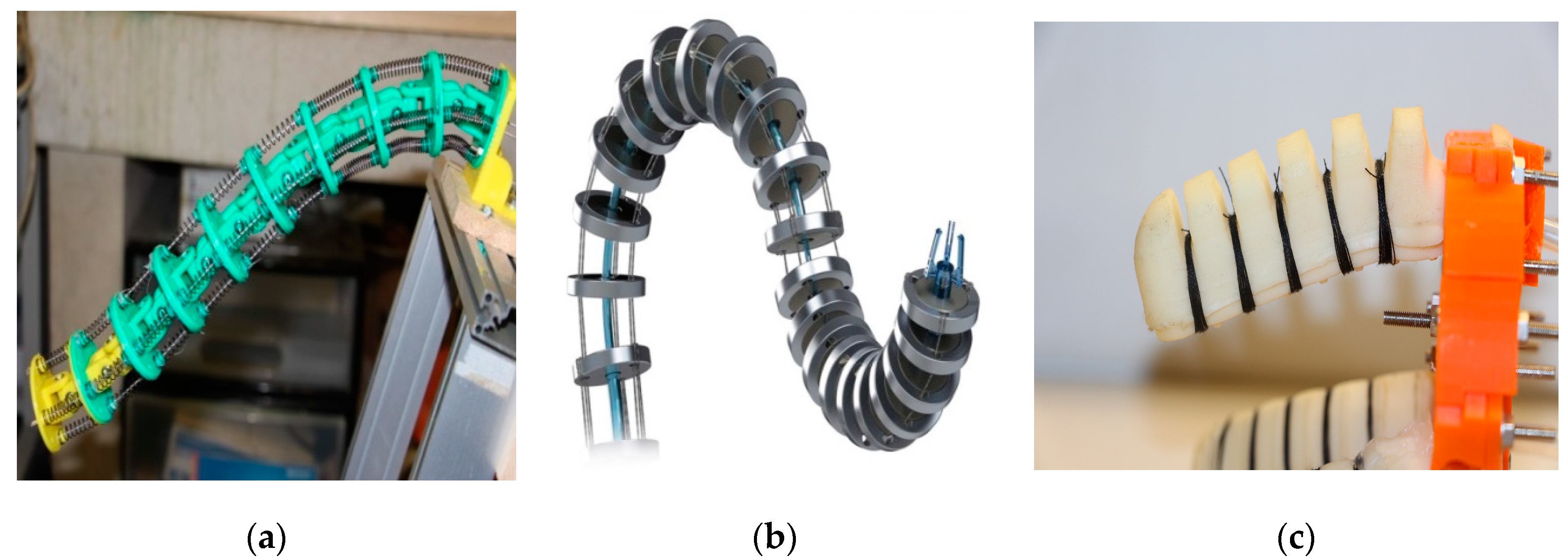
2. Related Work
3. Design Concept
3.1. Application Analysis
- Flexible dexterity: The robot should work in an unstructured workspace.
- Obstacle avoidance capability: The robot should avoid contact with solid surfaces and not collide with them.
- Reachability: The robot should possess as much reachable configuration as possible in spite of a narrow space and obstacles.
- Safety: The robot should be safe enough to avoid breaking any parts of the plant.
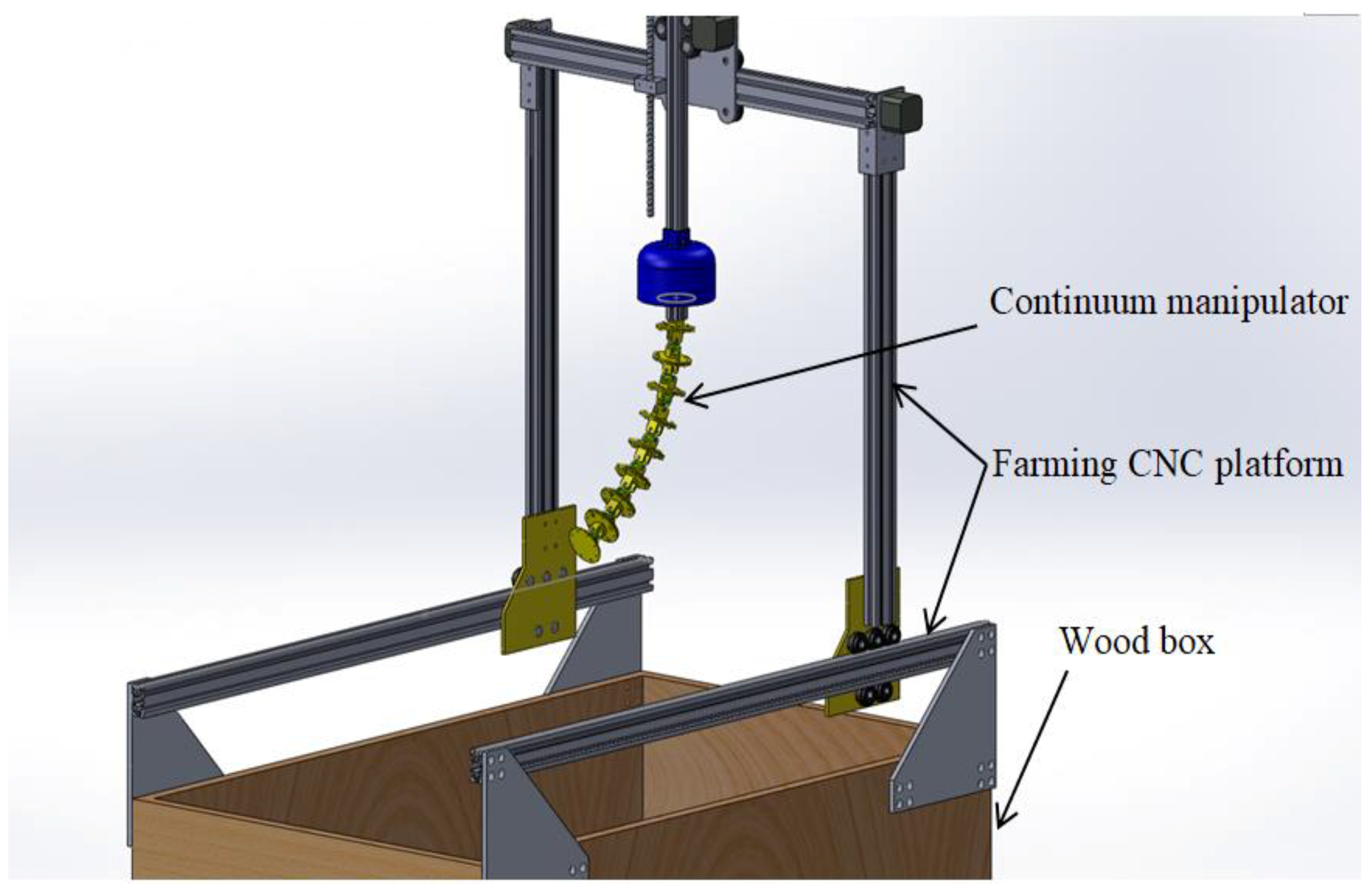
- Portability: The robot should be compact enough to be used as a tool in the farming CNC platform (see Figure 3).
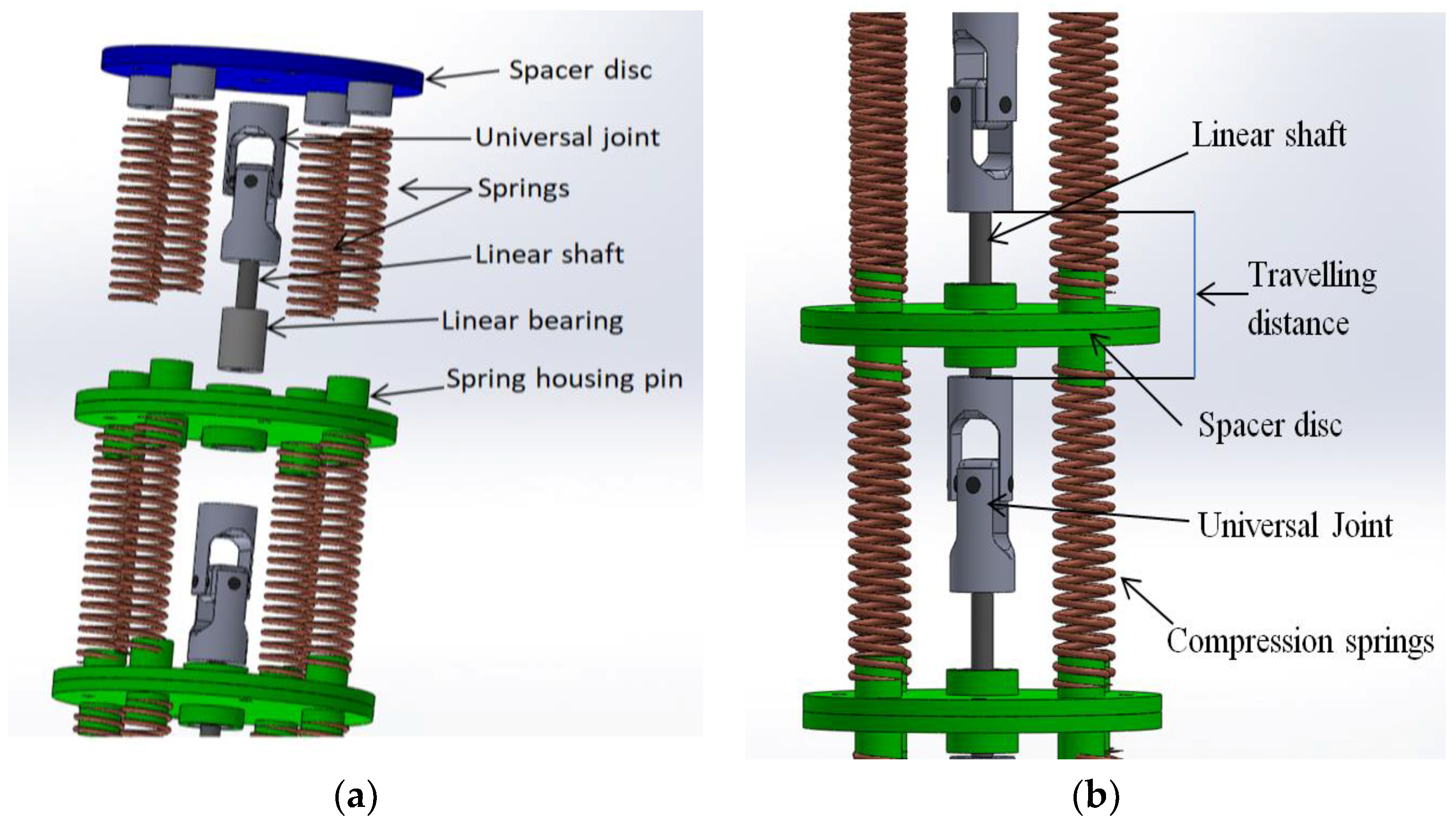
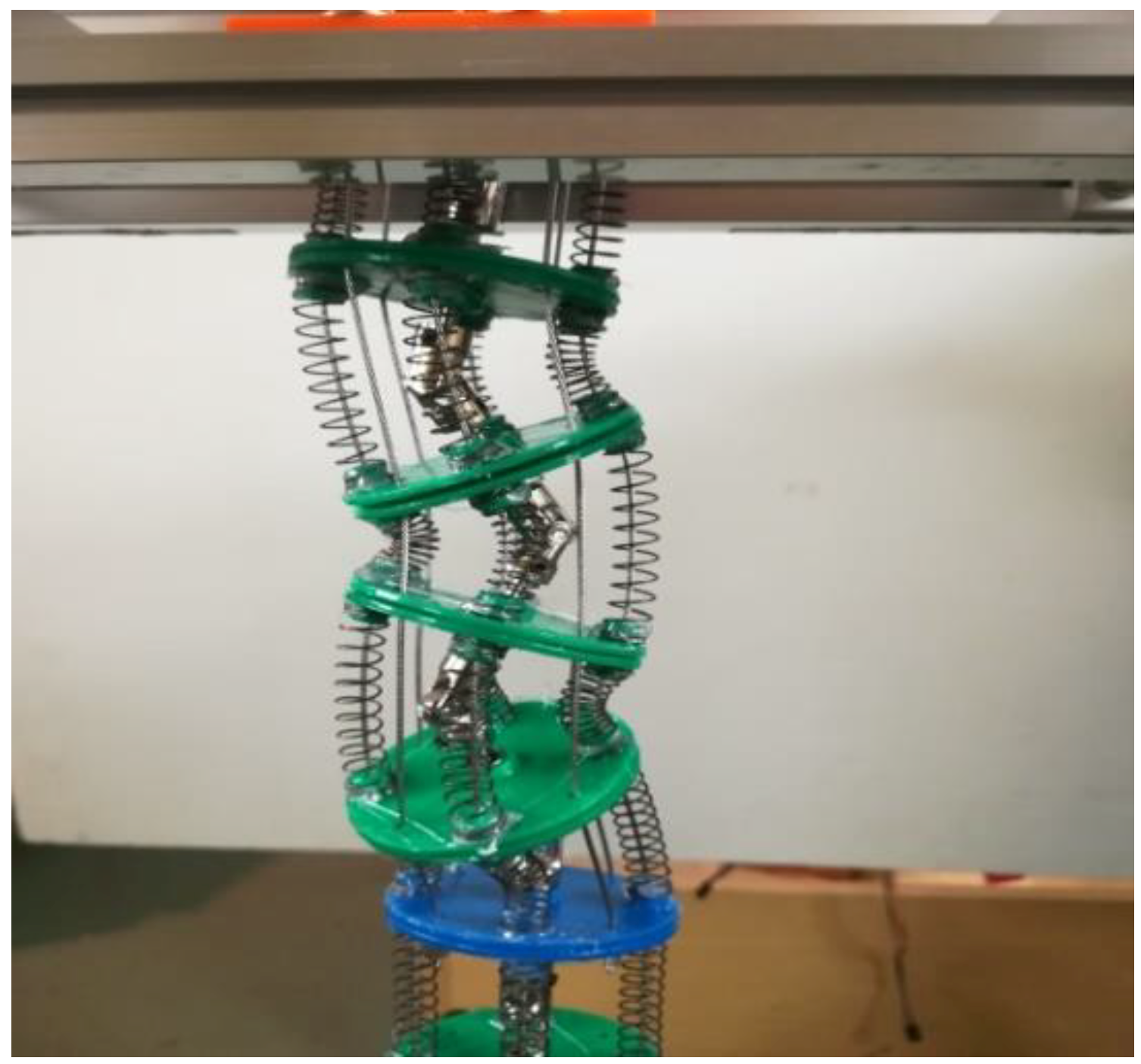
3.2. Sliding Disc Mechanism
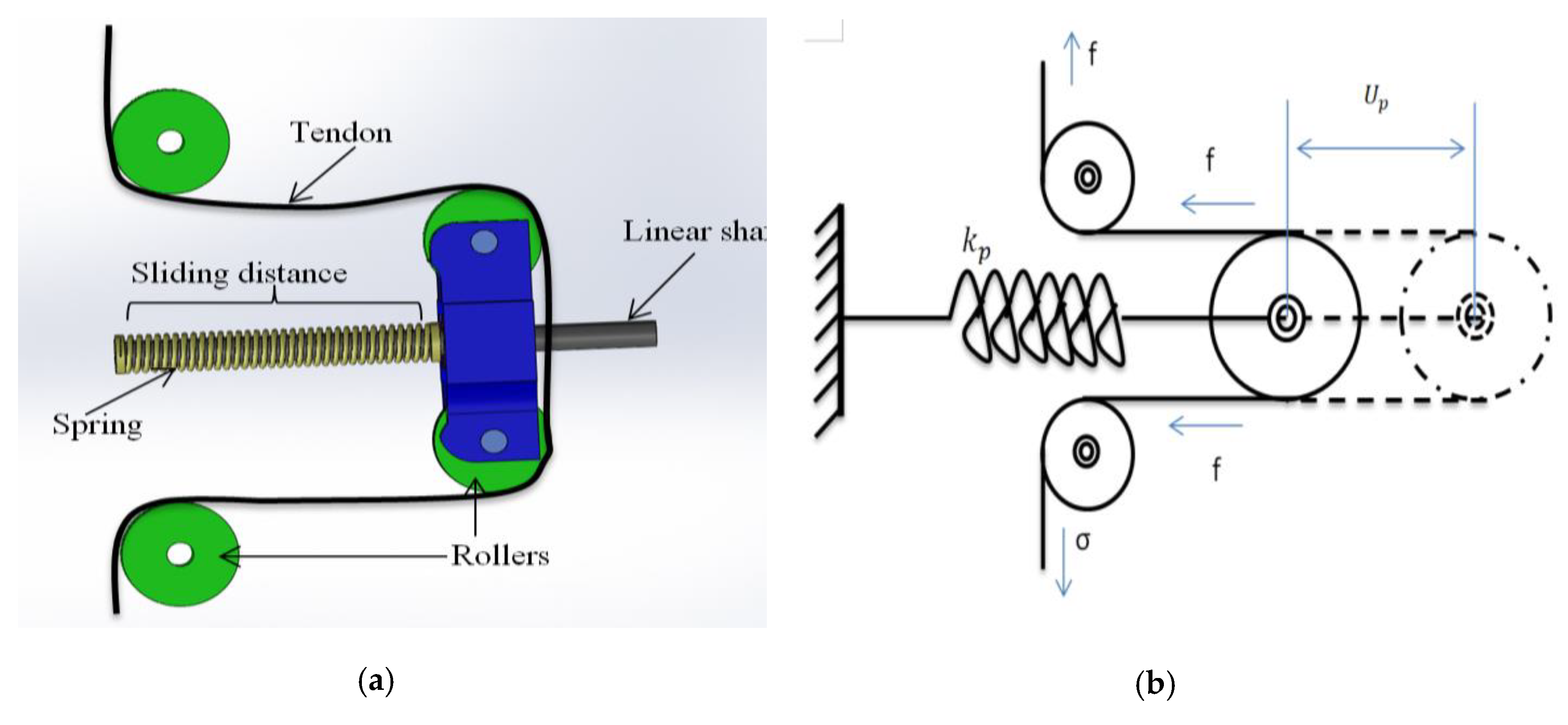
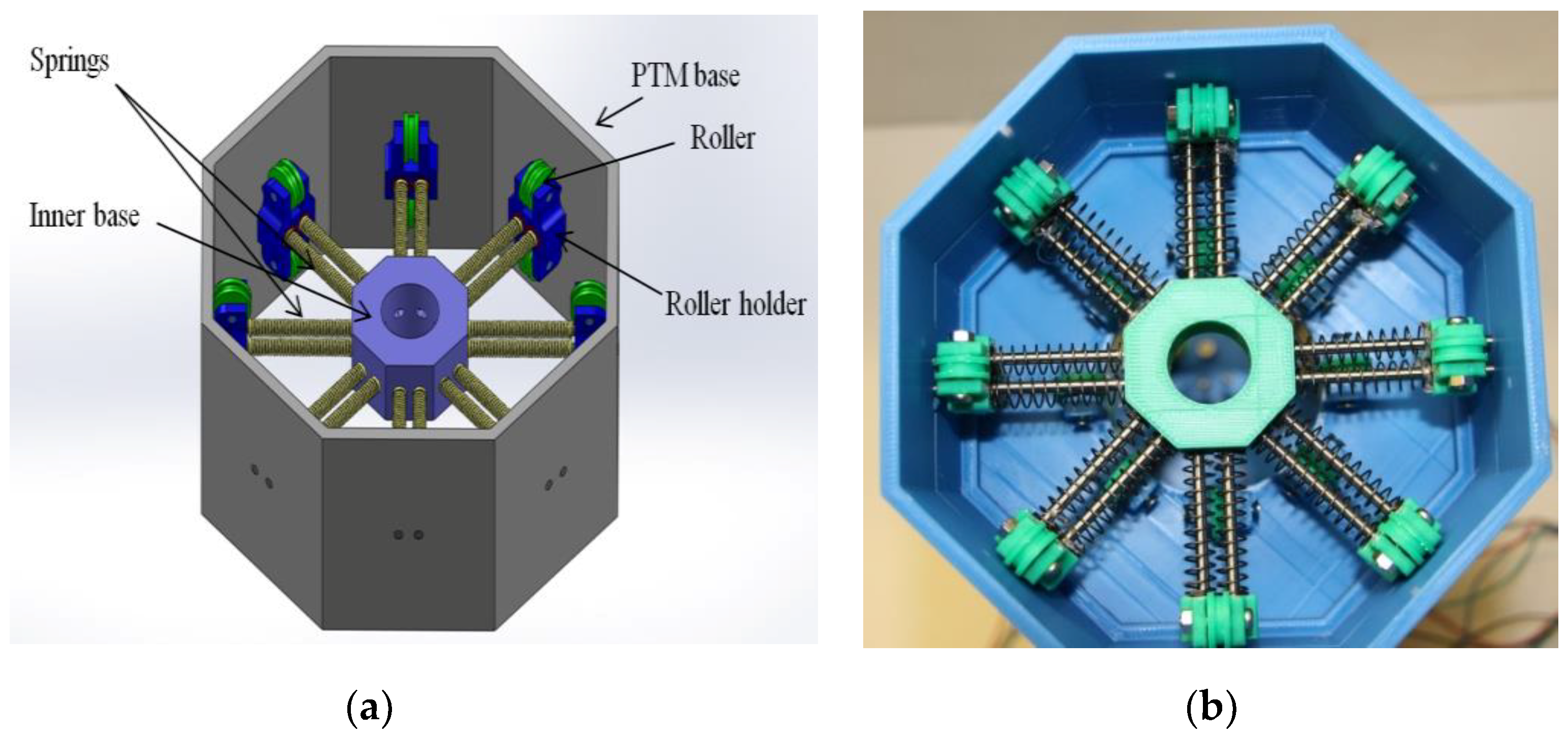
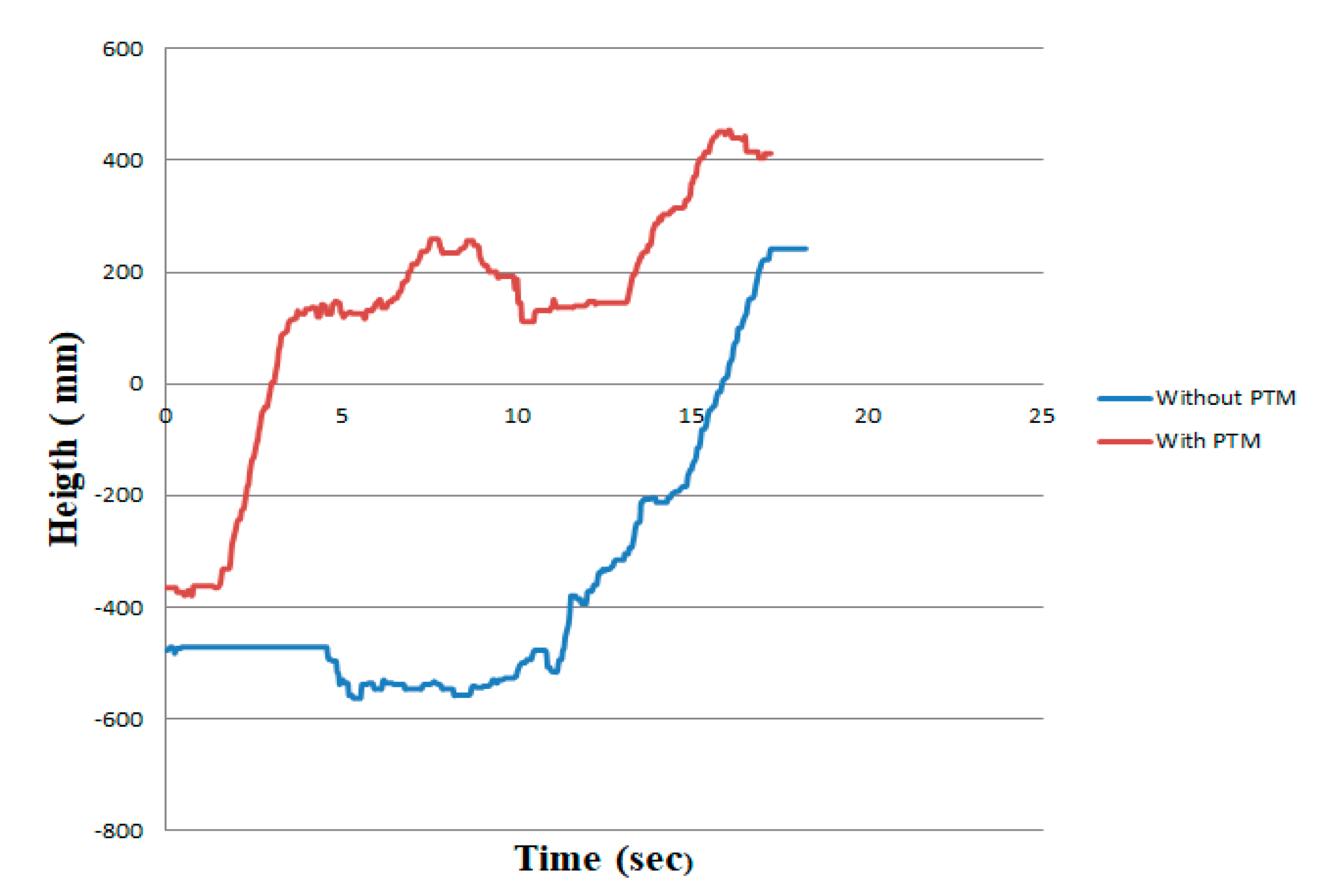
3.3. Pretension Mechanism Design
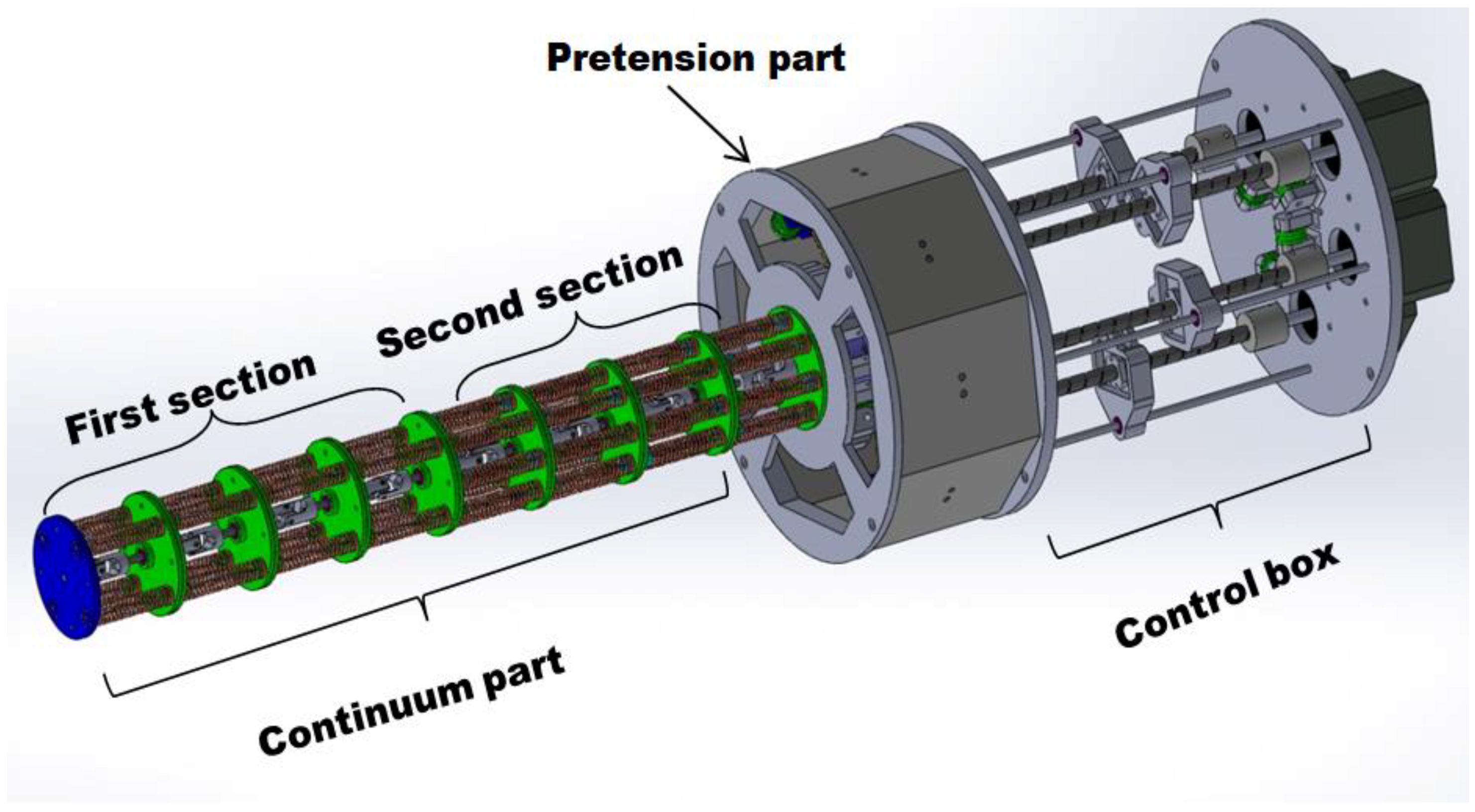
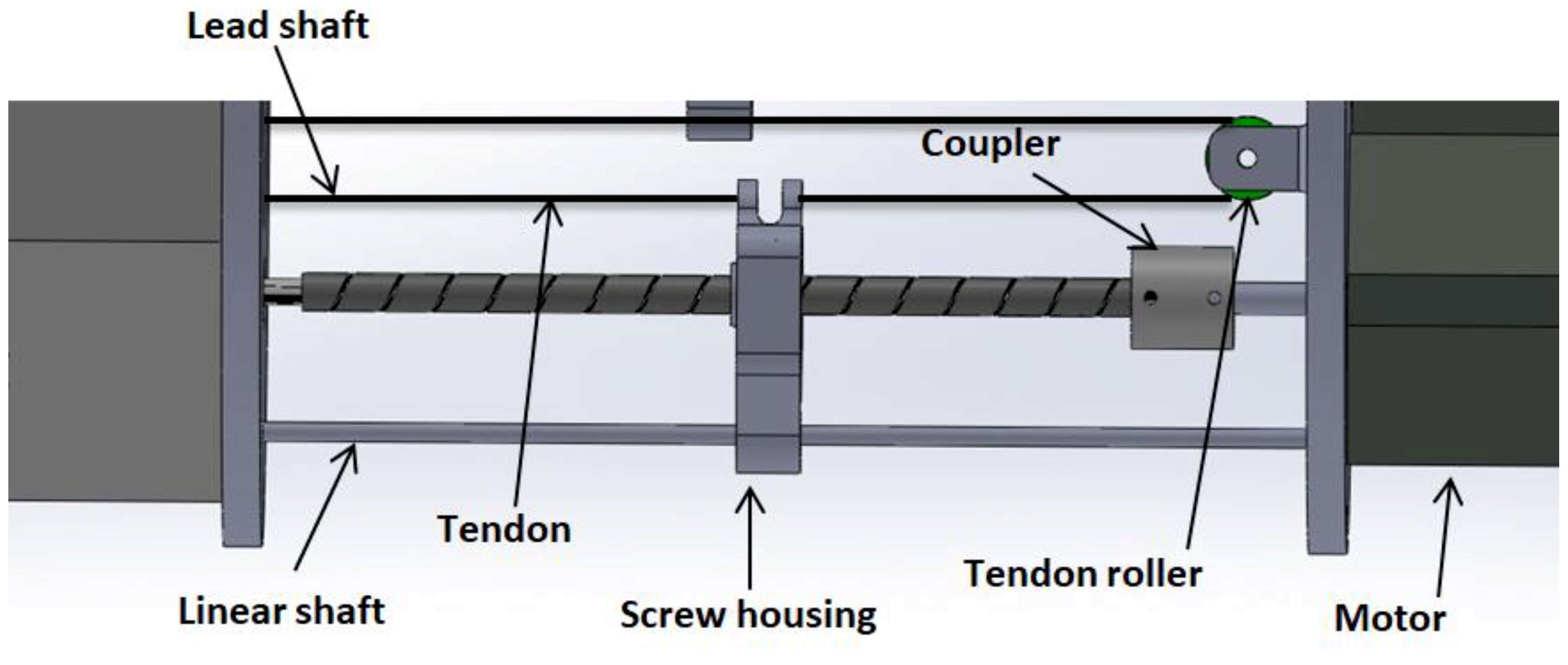
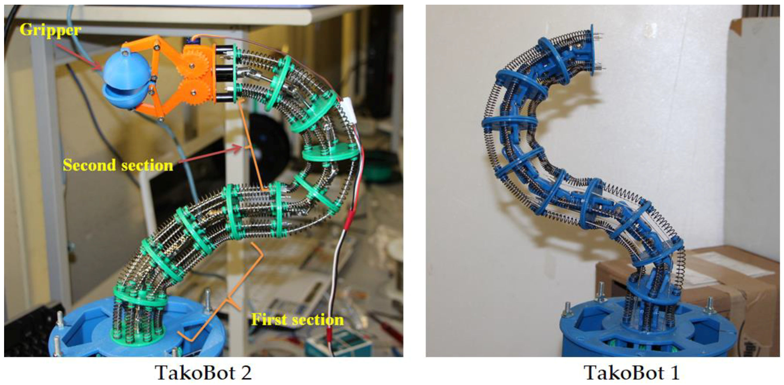
3.4. Robot Actuating Unit
4. Kinematic and Kinetic Formulation
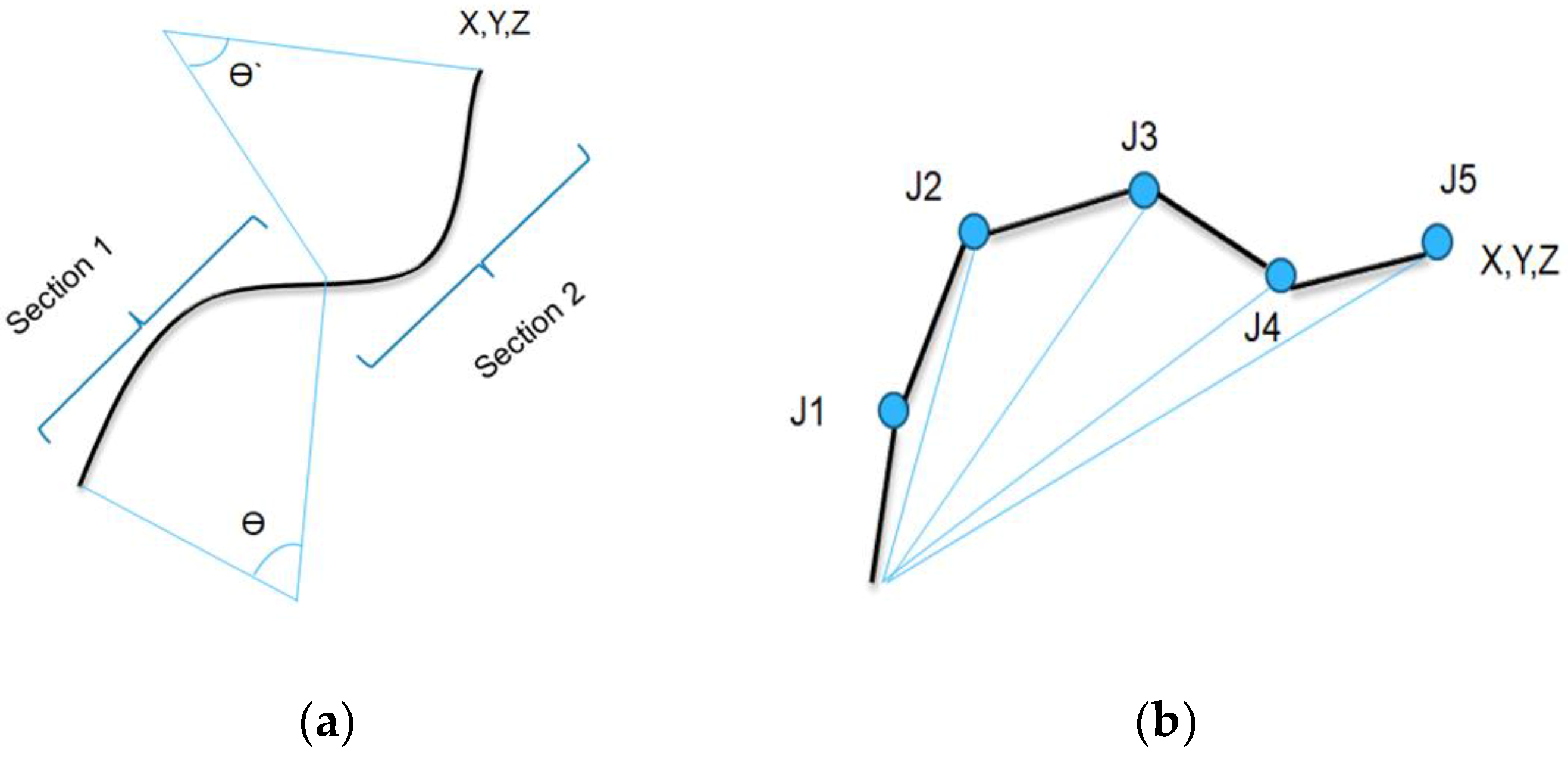
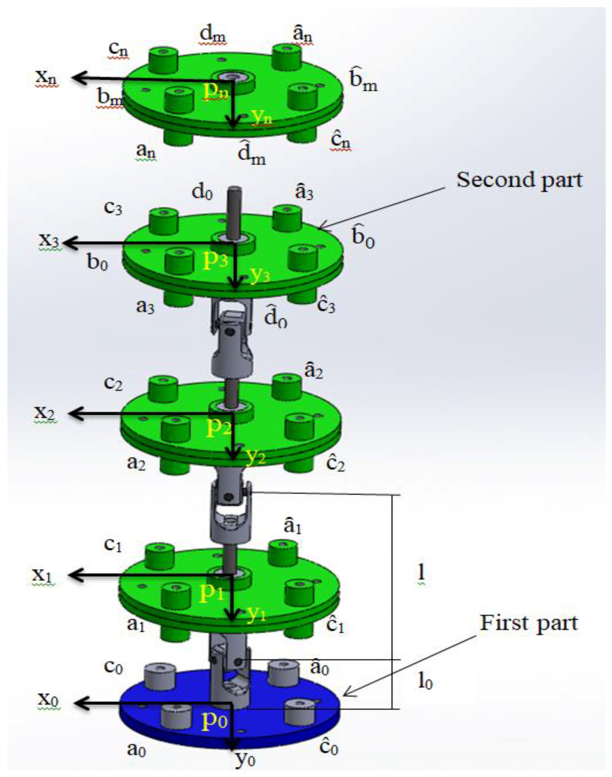
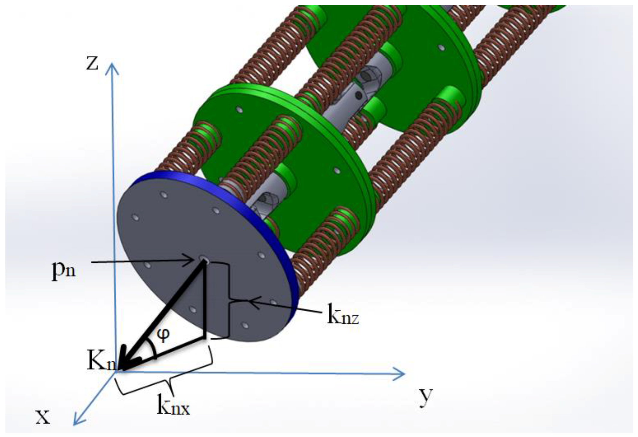
4.1. Forward Kinematic Formulation
4.2. Kinetic Formulation
4.3. Pretention Mechanism Formulation
4.4. Inverse Solution and Control
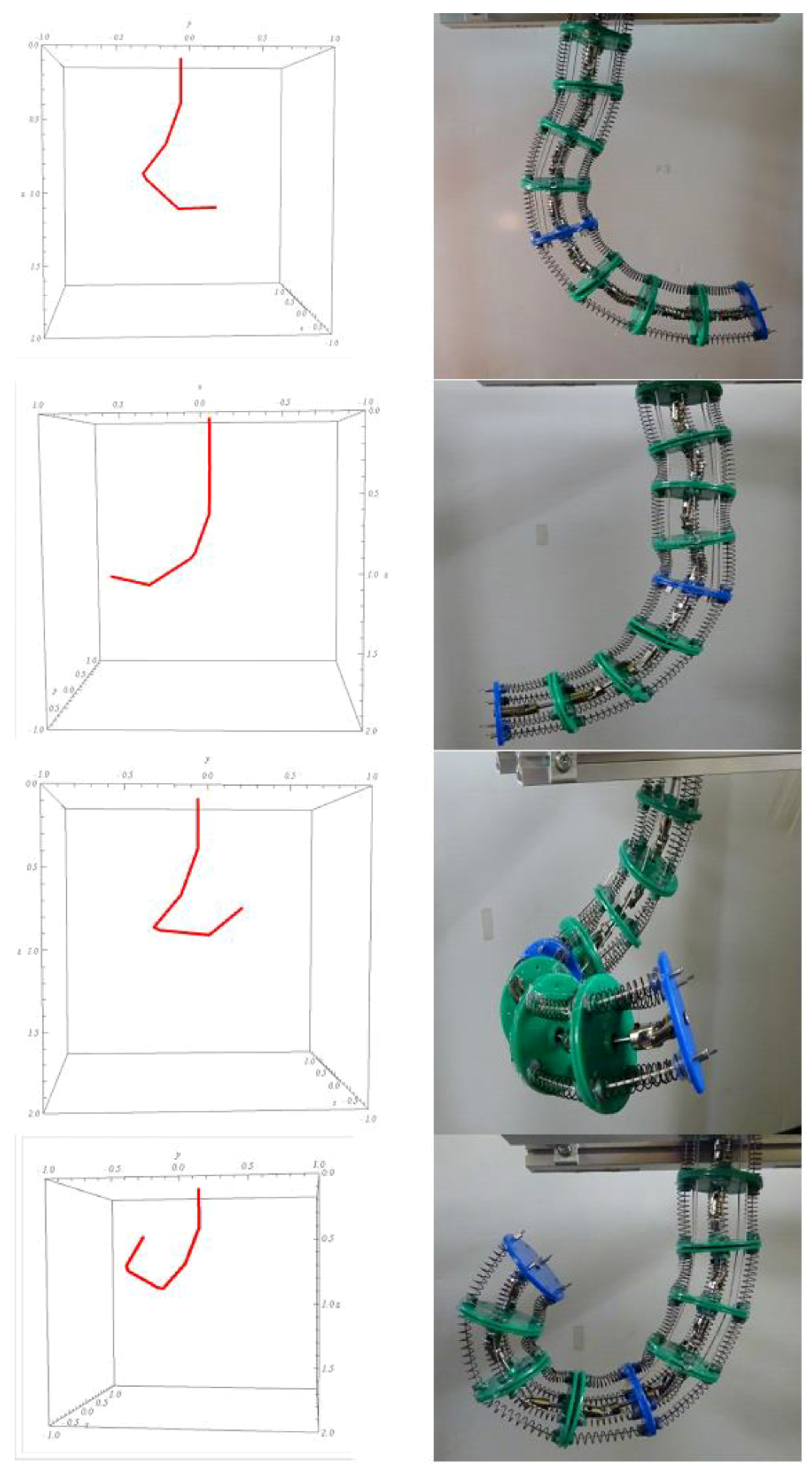
5. Experiment and Simulation
6. Conclusions
Supplementary Materials
Author Contributions
Funding
Conflicts of Interest
References
- In, H.K.; Kang, S.K.; Cho, K.J. Capstan Brake: Passive Brake for Tendon-Driven Mechanism. In Proceedings of the 2012 IEEE/RSJ International Conference on Intelligent Robots and Systems, Vilamoura, Portugal, 7–12 October 2012; pp. 2301–2306. [Google Scholar]
- Haiya, K.; Komada, S.; Hirai, J. Tension control for Tendon Mechanisms by Compensation of Nonlinear Spring Characteristic Equation Error. In Proceedings of the 2010 IEEE International Workshop on Advanced Motion Control, Nagaoka, Japan, 21–24 March 2010; pp. 42–47. [Google Scholar]
- In, H.; Lee, H.; Jeong, U.; Kang, B.B.; Cho, K.J. Feasibility study of a slack enabling actuator for actuating tendon-driven soft wearable robot without pretension. In Proceedings of the 2015 IEEE International Conference on Robotics and Automation (ICRA), Seattle, WA, USA, 26–30 May 2015; pp. 1229–1234. [Google Scholar]
- Tang, N.; Gu, X.; Ren, H. Design, characterization and applications of a novel soft actuator driven by flexible shafts. Mech. Mach. Theory 2018, 122, 197–218. [Google Scholar]
- Webster, R.J.; Jones, B.A. Design and kinematic modelling of constant curvature continuum robots: A review. Int. J. Robot. Res. 2010, 29, 1661–1683. [Google Scholar] [CrossRef]
- Yeshmukhametov, A.; Koganezawa, K.; Yamamoto, Y. Design and Kinematics of Cable-Driven Continuum Robot Arm with Universal Joint Backbone. In Proceedings of the IEEE International Conference on Robotics and Biomimetics, Kuala Lumpur, Malaysia, 12–15 December 2018; pp. 2444–2449. [Google Scholar]
- Seume, J. Researching the supreme discipline together. AEROPORT, The aviation magazine of MTU Aero Engines. 2017, Volume 01/17. Available online: www.aeroreport.du (accessed on 6 June 2019).
- Anderson, V.C.; Horn, R.C. Tensor arm manipulator design. Trans. ASME 1967, 67, 1–12. [Google Scholar]
- Lane, D.M.; Davies, J.B.C.; Robinson, G.; O’Brian, D.J. The Amadeus dexterous subsea hand: Design modelling, and sensor processing. IEEE J. Oceanic Eng. 1999, 24, 96–111. [Google Scholar] [CrossRef]
- Suzumori, K.; Iikira, S.; Tanaka, H. Development of flexible microactuator and its applications to robotic mechanisms. In Proceedings of the IEEE International Conference on Robotics and Automation, Sacramento, CA, USA, 9–11 April 1991; pp. 1622–1627. [Google Scholar]
- Wilson, J.F.; Li, D.; Chen, Z.; George, R.T. Flexible robot manipulators and grippers: Relatives of elephant trunks and squid tentacles. In Robots and Biological Systems: Towards a New Bionics? Springer: Berlin/Heidelberg, Germany, 1993; Volume 102, pp. 474–479. [Google Scholar]
- Aoki, T.; Ochiai, A.; Hirose, S. Study on slime robot development of the mobile robot prototype model using bridle bellows. In Proceedings of the IEEE International Conference on Robotics and Automation, New Orleans, LA, USA, 26 April–1 May 2004; pp. 2808–2813. [Google Scholar]
- Robinson, G.; Davies, J.B.C. Continuum robots-a state of the art. In Proceedings of the 1999 IEEE International Conference on Robotics and Automation (Cat. No.99CH36288C), Detroit, MI, USA, 10–15 May 1999; pp. 2849–2854. [Google Scholar]
- Degani, A.; Choset, H.; Wolf, A.; Zenati, M.A. Highly articulated robotic probe for minimally invasive surgery. In Proceedings of the IEEE International Conference on Robotics and Automation, Orlando, FL, USA, 15–19 May 2006; pp. 4167–4172. [Google Scholar]
- Li, Z.; Feeling, J.; Ren, H.; Yu, H. A Novel Tele-Operated Flexible Robot Targeted for Minimally Invasive Robotic Surgery. Engineering 2015, 1, 73–78. [Google Scholar] [CrossRef]
- Kang, B.; Koijev, R.; Sinibaldi, E. The First Interlaced Continuum Robot, Devised to Intrinsically Follow the Leader. PLoS ONE 2016, 11, e0150278. [Google Scholar] [CrossRef] [PubMed][Green Version]
- Ji, D.; Kang, T.H.; Shim, S.; Lee, S.; Hong, J. Wire-driven flexible manipulator with constrained spherical joints for minimally invasive surgery. In International Journal of Computer Assisted Radiology and Surgery; Springer: Berlin, Germany, 2019; pp. 1–13. [Google Scholar]
- Zhao, B.; Zhang, W.; Zhang, Z.; Zhu, X.; Xu, K. Continuum Manipulator with Redundant Backbones and Constrained Bending Curvature for Continuously Variable Stiffness. In Proceedings of the IEEE International Conference on Intelligent Robots and Systems (IROS), Madrid, Spain, 1–5 October 2018; pp. 7492–7499. [Google Scholar]
- Li, Z.; Du, R. Design and analysis of a bio-inspired wire-driven multi-section flexible robot. Int. J Adv. Robots Syst. 2013, 10, 1–9. [Google Scholar] [CrossRef]
- Dong, X.; Axinte, D.; Palmer, D.; Cobos, S.; Rafles, M.; Rabani, A.; Kell, J. Development of a slender continuum robotic system for on-wing inspection/repair of gas turbine engines. Rob. Comput. Integr. Manuf. 2017, 44, 218–229. [Google Scholar] [CrossRef]


© 2019 by the authors. Licensee MDPI, Basel, Switzerland. This article is an open access article distributed under the terms and conditions of the Creative Commons Attribution (CC BY) license (http://creativecommons.org/licenses/by/4.0/).
Share and Cite
Yeshmukhametov, A.; Koganezawa, K.; Yamamoto, Y. A Novel Discrete Wire-Driven Continuum Robot Arm with Passive Sliding Disc: Design, Kinematics and Passive Tension Control. Robotics 2019, 8, 51. https://doi.org/10.3390/robotics8030051
Yeshmukhametov A, Koganezawa K, Yamamoto Y. A Novel Discrete Wire-Driven Continuum Robot Arm with Passive Sliding Disc: Design, Kinematics and Passive Tension Control. Robotics. 2019; 8(3):51. https://doi.org/10.3390/robotics8030051
Chicago/Turabian StyleYeshmukhametov, Azamat, Koichi Koganezawa, and Yoshio Yamamoto. 2019. "A Novel Discrete Wire-Driven Continuum Robot Arm with Passive Sliding Disc: Design, Kinematics and Passive Tension Control" Robotics 8, no. 3: 51. https://doi.org/10.3390/robotics8030051
APA StyleYeshmukhametov, A., Koganezawa, K., & Yamamoto, Y. (2019). A Novel Discrete Wire-Driven Continuum Robot Arm with Passive Sliding Disc: Design, Kinematics and Passive Tension Control. Robotics, 8(3), 51. https://doi.org/10.3390/robotics8030051