1. Autonomous Underwater Vehicles
1.1. Introduction
Autonomous underwater vehicles (AUVs) are a sub-group of unmanned undersea vehicles (UUVs), which have changed the way marine environment is surveyed, monitored, and mapped. Autonomous underwater vehicles have a wide range of applications in research, military, and commercial settings. Especially, the oil and gas industry shows great interest in using autonomous underwater vehicles for finding new underwater oil fields and for pipeline inspection [
1]. They are utilised when the use of manned undersea vehicles is too dangerous, impossible, or too expensive [
2]. In general, AUVs not only perform a given task but also adapt to changes in the environment [
3]. In the underwater surroundings, typical influences are sudden side currents, downdrafts, and other effects, which are extremely unpredictable. To navigate properly, these effects need to be detected.
1.2. Underwater Navigation
Typically, an AUV uses dead reckoning, e.g., Doppler velocity log [
4], and some form of inertial measurement unit (IMU) to obtain its current position. High-end IMUs with fibre optic gyroscope have a sensor drift of about
/h (recently developed instruments show a sensor drift that is even as low as
/h [
5]) which translates into a positional error of less than 100 m per hour [
6]. Further technologies in use are sonars, pressure sensors, compasses, magnetometers, and cameras [
5]. Sonars currently have an along-track resolution of
to
and a cross-track resolution of 5 cm to 10 cm [
7]. Pressure sensors are only used to determine the underwater depth at the moment [
8] with an accuracy of about 10 cm. Compasses (accuracy
to
[
5]) and magnetometers require a good knowledge of the local magnetic field. Cameras are quite accurate but only work close to the sea floor. An extensive review on AUV navigation and localisation can be found in Paull et al. [
5].
In the past years, there has also been research towards the use of multiple pressure sensors for underwater navigation [
9]. Inspired by the lateral-line of fish, pressure sensors are placed along lines on the sides of underwater robots to register obstacles in the environment [
10,
11]. Recently, it has been demonstrated that robots can successfully navigate along walls making use of pressure variations due to the wall effect [
12]. Wall detection with differential pressure sensors (DPS) was also achieved by Xu and Mohseni [
13]. Pressure sensors have the advantage of requiring almost no power to operate and can be placed easily on the surface of existing AUVs [
14,
15].
A different approach with multiple pressure sensors was taken by Shang et al. [
8] who used an array constituting four pressure sensors. The four sensors are placed on the AUV’s surface at the top, bottom, and the two sides at the centroid. This allows the estimation of the attitude of the AUV with an extended Kalman filter (EKF).
Various systems are usually combined by means of sensor fusion algorithms [
16,
17]. This way the position of the AUV can be determined quite accurately.
1.3. Determination of Sea Current
Except for the pressure sensors, however, the disturbances in the water flow are not measured using the systems mentioned above. Only the indirect effects, e.g., a change in acceleration, can be observed.
Computational fluid dynamics (CFD) was already used by Suzuki et al. [
18] to obtain hydrodynamic force coefficients of an AUV. However, a reverse solution allowing the determination of the flow parameters from the hydrodynamic force coefficients was not available at this point. Li et al. [
19] established that it is in principle possible to determine the attitude of an AUV from pressure data with the help of a CFD-based hydrodynamic model.
Bayat et al. [
20] addressed the problem of localising an AUV under the influence of unknown currents. The unknown currents are assumed to be constant. It is shown that the system becomes observable under the influence of these currents once depth measurements are available, hence making a compensation possible in this case.
In [
21], an onboard acoustic Doppler current profiler (ADCP) is used to measure the currents in the vicinity of an AUV. The method is shown to be very accurate. However, due to the sensor’s capabilities, not the actual current experienced by the AUV is determined, but the current at a distance of a few meters.
Osborn et al. [
22] applied an EKF to estimate the north and east component of the current. It is shown that the estimation is accurate in simulations even when the AUV changes direction.
An unscented Kalman filter (UKF) was used by Allotta et al. [
23] to estimate the current experienced by an AUV which is assumed to be uniform. The current estimation is based on an extended model of the vehicle dynamics including sea current. The estimate is then obtained by regarding the available data from all sensors.
Pressure sensors have also been applied successfully to detect currents. Kottapalli et al. [
15] used the artificial lateral-lines mentioned above to determine the velocity of an oncoming flow. Gao and Triantafyllou [
24] obtained the angle of attack and its change of an oncoming flow through the pressure information of artificial lateral-lines.
As an alternative, differential pressure sensors have been shown to allow the extraction of the flow velocity in changing flows with high accuracy [
25,
26]. As in [
15], the approach is limited to oncoming flow. However, it allows for different angles of attack as in [
24].
1.4. Motivation and Objective
It is of interest to detect the disturbances directly through measurements in order to increase the accuracy and reliability of the navigation systems of an AUV. This is essential in order to allow the use of simultaneous localisation and mapping (SLAM) algorithms. These measurements should be independent of the availability of depth information, as in [
20].
As the disturbances yield an instantaneous change of the pressure that is exerted on the surface of the AUV’s body, it is proposed to place sensors at specific points on the AUV’s body to measure the pressure at these positions. The proposed configuration is based on artificial lateral-lines with additional pressure sensors at the top and bottom of the AUV. Details are given in
Section 3.3. In contrast to Williams et al. [
21], this would provide information on the actual disturbances experienced by the AUV. Furthermore, an ADCP is a lot more expensive than several pressure sensors, possibly reducing the sensor costs significantly.
In this study, how machine learning can be used to obtain flow parameters of the surrounding fluid from pressure data and which machine learning algorithms are appropriate for this task were investigated. Determining flow parameters from pressure is the reverse of the standard method (as mentioned above with regard to Suzuki et al. [
18]) where the flow parameters are known and the pressure distribution is calculated.
It was already shown that this reversal is possible for the velocity and aspect angle of an oncoming flow. However, for a flow from any direction, this has not been done to our knowledge. It is believed that machine learning methods are particularly suitable for this task as the relation between pressure and flow velocity is quite complex for a general flow situation.
This approach could for instance be used to supplement the sensor data in [
23], making it more robust. To this end, an extensive number of different flow situations are simulated applying CFD, the pressure distribution and the flow parameters are obtained, and analysed using different learning algorithms.
2. Machine Learning
In this section, the machine learning procedures used in this study are briefly introduced. For more details, it is recommended to follow the references provided.
2.1. Artificial Neural Network (ANN)
Artificial neural networks are information processing algorithms that are modelled after the way brains work [
27]. The first formulations of this method were already made in 1943 by McCulloch and Pitts [
28].
Artificial neural networks are widely used in marine contexts. They can, for instance, be applied to minimise the electric field in current cathodic protection systems [
29]. In the underwater environment, artificial neural networks are often tasked with the improvement and analysis of underwater imagery. Examples include the reconstruction of low light images [
30] and the classification of sonar images [
31]. For underwater robots important uses of artificial neural networks are navigation and control. Current examples are the localisation of an underwater robot considering unmodelled noise [
32] and the target tracking of underactuated AUVs [
33].
Neural networks consist of strongly interconnected nodes called neurons. These neurons are organised as layers: one input layer, one output layer, and one or more hidden layers in-between. The number of nodes in the input and output layer is given due to the nature of the data being processed. Within this work, there are three nodes in the output layer to represent the translational velocities along the three axes of a Cartesian coordinate system. The number of nodes in the input layer depends on the number of points on the AUV at which the surface pressure is obtained. The number of nodes in the hidden layers as well as the number of hidden layers is variable [
34].
Data
that are passed from one node
i to the next node
j are weighted (weight
, can be positive or negative). In addition, every node has a bias
, which can also be positive or negative. The input
to node
j is therefore [
35]
The output
of node
j is then some function
of the input
.
is called the activation function of the artificial neuron. There are essentially two fundamental types of activation functions [
35]. On the one hand, threshold functions may be used where the neuron is either activated or not. On the other hand, it may be desirable to have a smooth transition between the two states “node not active” and “node active”. In this case, sigmoid functions are used.
With this method, it is possible to obtain patterns and information from complex data. Further advantages of artificial neural networks are adaptive learning, self-organisation, real time operation, and fault tolerance [
27].
Teaching neural networks is done by forming or removing connections, changing the weights, changing the threshold of neurons, and adding or removing neurons in order to minimise errors for a given validation set. However, in many cases, the overall shape of the neural network is fixed and only the weights and thresholds are used for learning [
34]. A common method for training is the back-propagation algorithm which is also used in this study. Hereby, the error derivative of the weights, i.e., the change of error depending on the change of weight, is determined backwards by starting with the total error at the output layer and the moving through the network towards the input layer [
36]. This is done repeatedly until either the rate of change of the errors or the error derivatives become sufficiently small.
In this study, up to 250 learning cycles are used with a learning rate of 0.1 and a momentum of 0.2 for a given neuron configuration. The number of neurons was varied between and p (where p is the number of inputs) per layer with the number of layers between 1 and 4.
2.2. k-Nearest Neighbour (KNN)
k-nearest neighbour is a non-parametric method for classification and regression.
k-nearest neighbour is applied in medical contexts, e.g., for the classifications of electroencephalogram signals [
37]. They also have a range of applications in computer vision for the classification of images and objects therein [
38,
39].
The output (classification or property value) for a given input is obtained from known input–output relations where the inputs are similar and close to, i.e., “in the neighbourhood of”, the sample point in question. Classification is then done by majority voting and in case of a property value the average of the outputs of the neighbouring inputs is taken [
40]. In the case of this work, data points are situated in an
n-dimensional space, where
n is the number of points on the AUV at which the surface pressure is obtained.
Usually, the contributions of the neighbouring data points are weighted depending on the distance so that data points closer to the sample point have a stronger influence on the output. Typically, a type of exponential expression is used. Thus, if the neighbourhood
k contains data points
with weights
with respect to the sample point
, the value of the sample point can be obtained from [
41]
with
where
is the distance of data point
frTurbulence Modeling Validation, Testing, and Development. he sample point
.
The result depends on the choice of the neighbourhood, i.e., up to what distance or how many neighbours are taken into account. In addition, the type of distance measure (Euclidean, Manhattan, etc.) has some influence [
41]. Teaching a
k-nearest neighbour system is usually done by finding the size of the neighbourhood
k with the lowest error by cross-validation [
41].
2.3. Support Vector Machine (SVM)
Support vector machines are non-probabilistic linear classifiers. However, they can also be used for regression [
42]. The fundamental idea is that datasets that belong to different classes are linearly separable by hyperplanes. If the data cannot be separated by linear hyperplanes, it has to be mapped into a higher dimensional (embedding) space such that it becomes linearly separable [
43].
Support vector machines are widely applied in medical research for classification of clinical pictures. Examples would be electroencephalogram signal classifications [
44]—as for KNN—or subtyping of cancer [
45]. However, they are also used in robotics for path planning [
46] and for the analysis of underwater images [
47].
Of all the hyperplanes in a support vector machine that separate the datasets, one hyperplane has to be chosen such that the margin separating different classes is a maximum. Those data points closest to the boundary and which are required to describe the hyperplane exactly are called support vectors. Hence, teaching a support vector machine is essentially an optimisation problem. To be more precise, it is a minimisation with constraints, since the inverse of the size of the margin is used for optimisation [
43,
48]. Thus, in the most basic case, one minimises
where
is the normal vector to the hyperplane with the constraints
where
are multi-dimensional vectors (data points),
b is the (signed) distance from the separating hyperplane and
depending on which side of the separating hyperplane
is situated. Essentially, Equation (
5) states that no data point should be inside the margin separating the classes.
However, the embedding space is usually of a much higher dimension than the original input space. In fact, the embedding space often has a dimensionality in the range of a million or more [
2,
49]. Solving this quadratic programming problem with a regular computer is not feasible. However, instead of looking at the primal problem, one can look at the equivalent dual problem which is much easier to handle. With some further simplification (so-called “kernel trick”) [
43], the problem becomes feasible.
As for k-nearest neighbour, the support vector machine in this study will start in an n-dimensional space. However, due to the likely non-linear separability, the resulting machine will have a much higher dimensionality.
SVMs with a Gaussian Kernel are considered to be the best choice for this study. Kernel parameter () is varied between 0.1 and 5.0 to obtain the spread with the lowest error. For the optimisation, the cost of misclassification is set to a moderate value of 1.0, the convergence tolerance is 0.0010, and the width of the -sensitive zone is set to .
2.4. Bayesian Networks (BN)
Bayesian networks are probabilistic graphical models based on Bayesian probability theory (T. Bayes 1763) [
50]. A Bayesian net describes how different states
of a system, represented as nodes of a graph are linked through probability, i.e., the net shows conditional inter-dependencies of variables via a directed acyclic graph [
51].
Bayesian networks are often used when dealing with large quantities of data, e.g., data mining [
52,
53]. They are also applied in medical contexts [
54] and robotics [
55]. For the latter, one should mention that in the underwater environment risk assessment with Bayesian networks is a current topic [
56,
57].
In a Bayesian network, there is a conditional probability distribution
for each node where
are the parent nodes of
. A unique joint probability distribution over the graph is then [
50]
Bayesian networks can be learned from available data. Various procedures are available for teaching, which are separated into two categories [
58,
59]:
Often, parameter learning and structure learning are combined so that parameter learning is a sub-process of structure learning (score-and-search-based approach) [
60]. In this study, hill climbing [
61] with an alpha parameter of 0.5 is used.
2.5. Multiple Linear Regression (MLR)
Multiple linear regression is very similar to linear regression. However, instead of having one independent variable as for linear regression the output
y depends on two or more (in general
p) independent variables
[
41], i.e., one has
where
and
are constants.
Multiple linear regressions have a wide range of applications from chemistry, e.g., calibration methods [
62], to material science (an example would be fatigue life evaluation as in [
63]). In the marine environment, MLR are also applied successfully. For instance, Ghorbani et al. used MLR for the prediction of wave parameters of the coast of Tasmania [
64]. The location of the impressed current cathodic protection anode for ships can also be optimised with MLR, as shown in [
29]. Research into underwater acoustic source localisation is also done using multiple linear regressions [
65]. In this study, there are three separate MLRs (one for each flow direction in the Cartesian coordinate system) with
p independent variables (the pressure at each of the
p measurement points).
Learning a multiple linear regression machine is done via the method of least squares. The best linear unbiased estimator is found according to the Gauss–Markov theorem:
where for a given dataset of size
n,
is the
vector of the dependent variable and
is the
data matrix of the independent variables. This way one obtains an equation for the estimated value
of the dependent variable
y:
3. Methods
3.1. Numerical Simulations
To test the proposition, a large number of CFD simulations were carried out with ANSYS CFX 15.0. This is an established method to generate an extensive evaluation and a high quality dataset. Because of the very complex and multi-dimensional data structure of the flow itself, CFD provides the only plausible method for generating and validating the data for the learning algorithms. Other theoretical physics-based models could, in this case, never reach the quality of the CFD data.
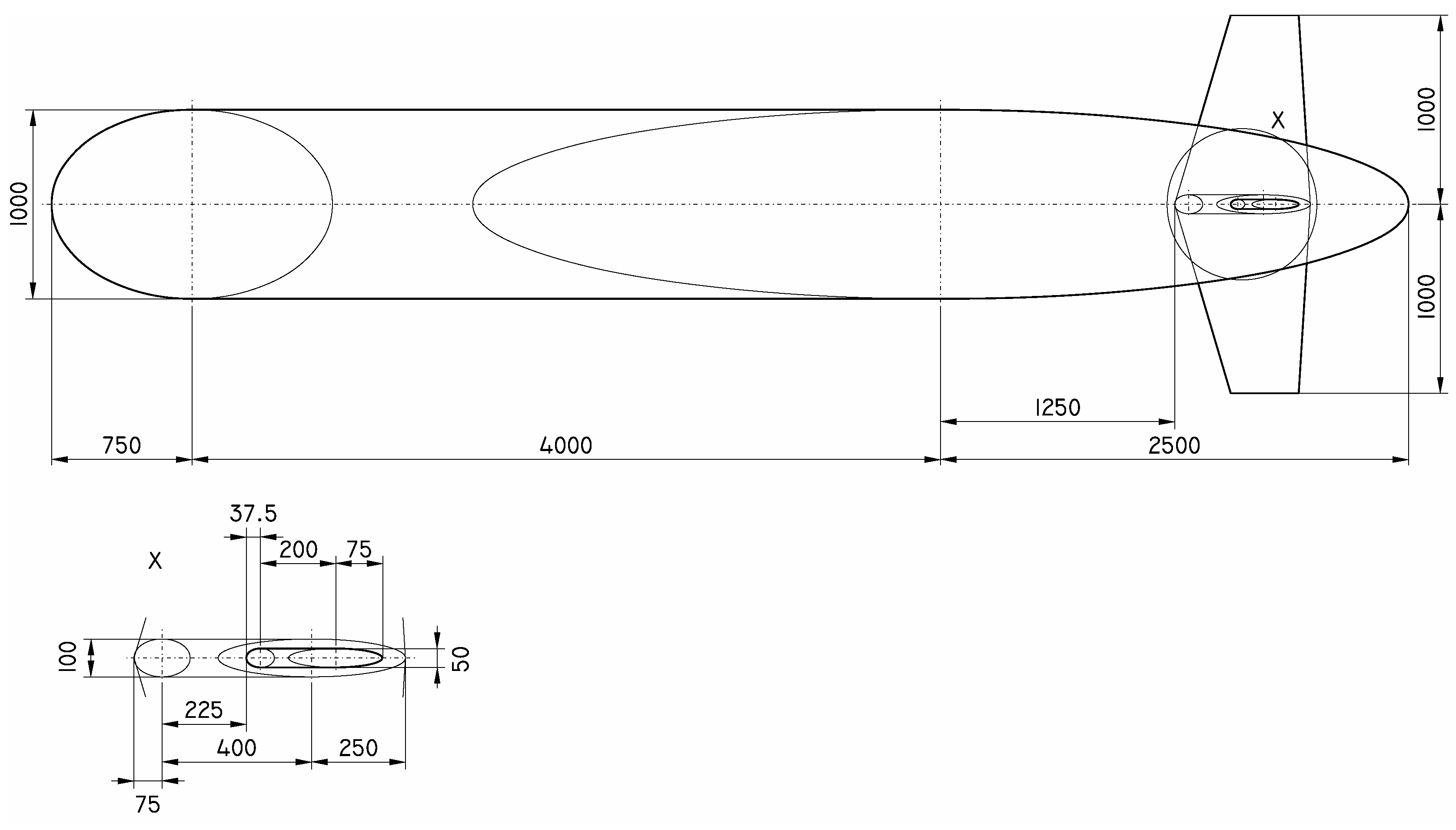
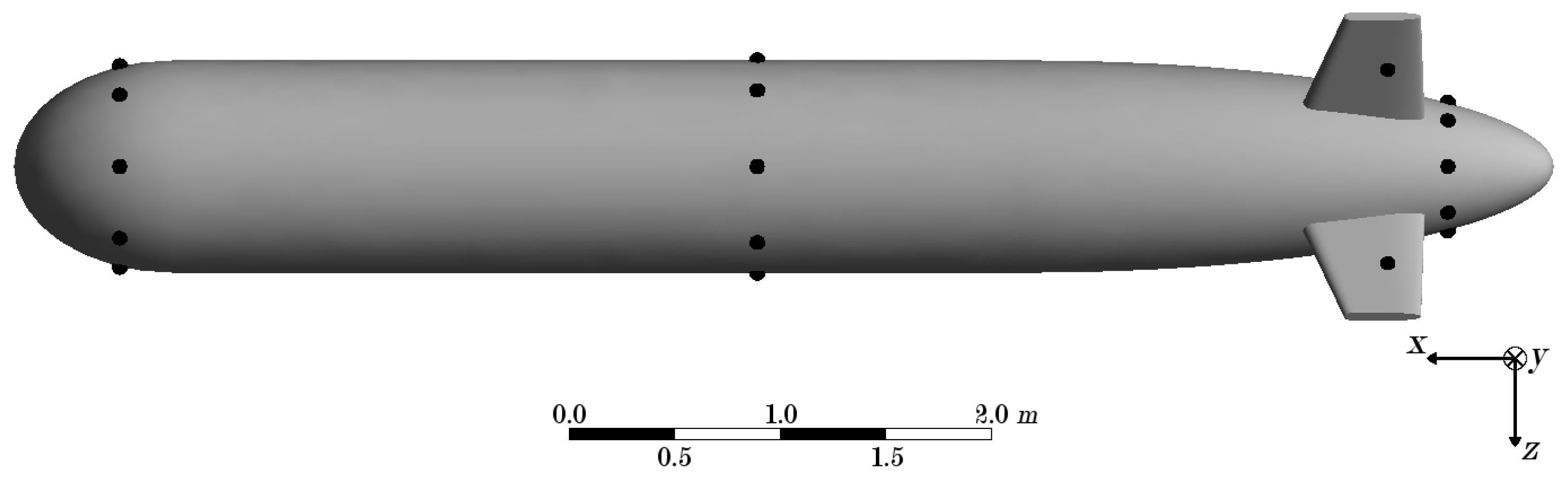
For the CFD simulations, a torpedo-shaped AUV body with a length overall of LOA = 7250 mm was used. A technical drawing of the AUV’s body can be found in
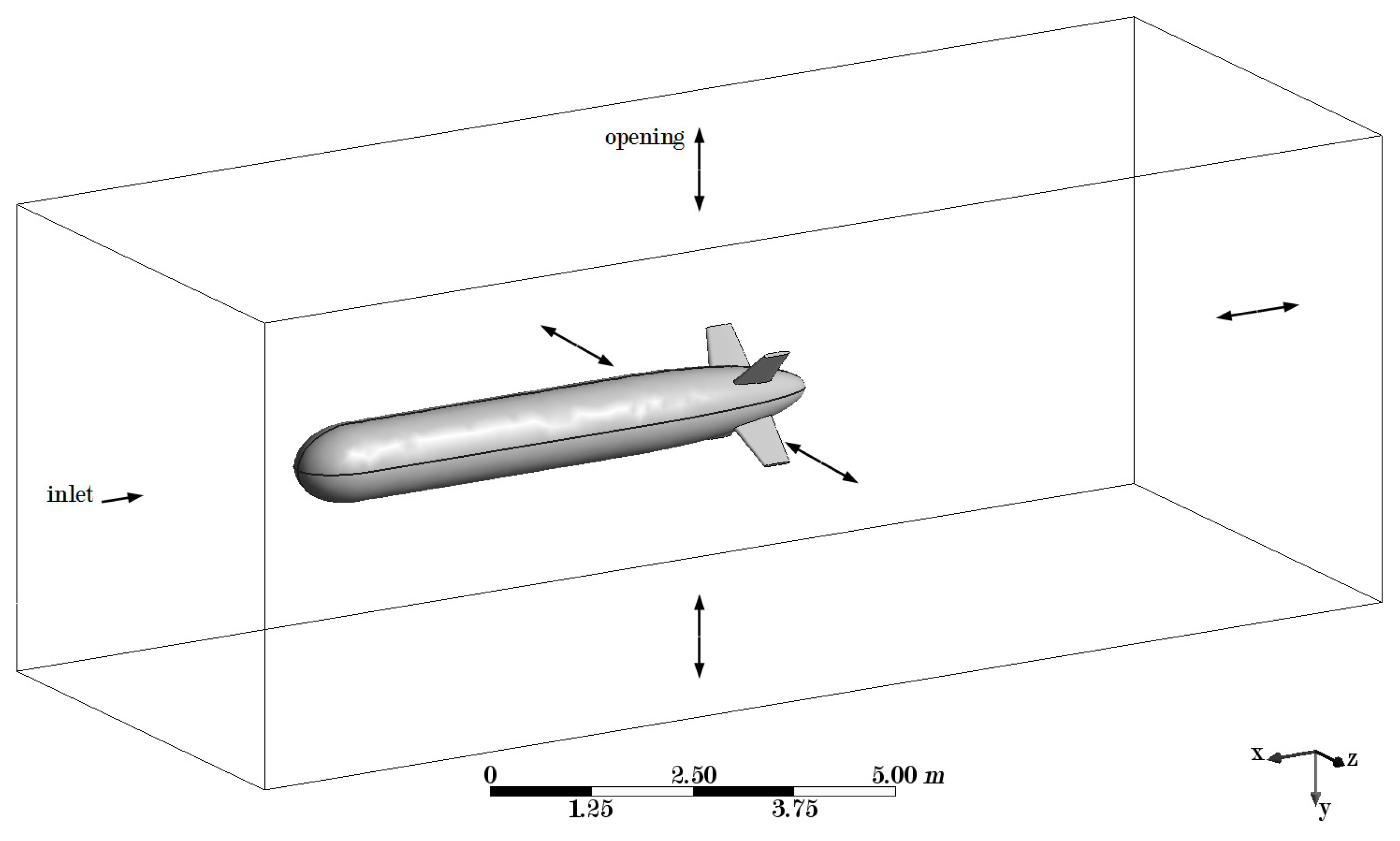
Figure 1. The fluid domain has a size of 16,000 mm × 6000 mm × 6000 mm (see
Figure 2). A pre-trail with high fluid velocities showed that this size is sufficient for the turbulence to dissipate before reaching the fluid boundaries.
The mesh has 92,819 nodes and 525,857 linear tetrahedral elements. A sensitivity analysis was performed and a finer mesh did not change the results of the simulations significantly.
For the fluid model, seawater at a salinity of
S = 35 g/kg and a temperature of
T = 15
C was chosen, which is typical for ocean water [
66,
67]. An isothermal
k-
-model with scalable wall functions was used and the reference pressure was set to
atm. This corresponds to the AUV being situated roughly 10 m below the surface of the water. Furthermore, the control volume was large enough that gravity would result in a significant difference in static pressure between its upper and lower side. Hence, buoyancy was also taken into account. In addition, no large adverse pressure gradients were expected and the
k-
-model works especially well for pressure gradients that are relatively small [
68]. The
k-
-model also provides a reasonable compromise between accuracy and computational effort [
69], in order to run the complete set of simulations within an adequate time frame.
The boundaries of the fluid domain were either inlets or openings depending on whether water was flowing in through the respective boundaries or not. The surface of the AUV was a no slip wall.
In total, 2873 simulations were performed with a large range of different flow situations. For the sideward, upward, and downward flow the velocities were between 0 kn and 5 kn; for the forward flow, the velocities were between 0 kn and 20 kn; and, for the backward flow, the velocities were again between 0 kn and 5 kn (see also
Table 1).
3.2. Governing Equations
For a mathematical model of fluid flow, the underlying principles are the conservation of mass and momentum [
40,
70]. Heat and mass transfer were not considered here as the temperature was uniform and no chemical reactions were taking place. These principles are expressed through the following equations. Continuity equation (conservation of mass):
Navier–Stokes equations (conservation of momentum):
In the equations above, is the fluid density, is the flow velocity vector (with components u, v, and w), p is the pressure, is the viscosity, is the vector of body forces per unit mass (buoyancy), and is the Kronecker tensor.
The
k-
model is a widely used two-equation turbulence model for fluid dynamical problems. It was introduced by B.E. Launder and D.B. Spalding [
69].
One defines the turbulent kinetic energy
k as the variance of the fluctuations in velocity.
where
,
, and
are the components of the velocity fluctuations
. Then,
is defined as the rate at which
k dissipates:
These variables are introduced in the continuity equation (Equation (
10)) and the Navier–Stokes equations (Equation (
11)). After some analytical manipulation, one obtains the following equations (as used in this study).
In these equations, is the turbulence production due to viscous forces and S is the modulus of the mean rate-of-strain tensor. and represent the influence of the buoyancy forces. , , , and are constants.
3.3. Data Processing
In a first step, the pressure was extracted at points 500 mm apart and situated on lines on the top, the bottom, and the two sides of the AUV (see black lines on the surface of the AUV in
Figure 2). This resulted in 14 points on each line and 56 points in total.
This setup was inspired by artificial lateral-lines. Since in a general flow situation there may also be a vertical flow velocity components, it is prudent to also have pressure sensors at the top and bottom of the AUV’s body. The separation—and hence the number—of pressure points is a compromise between obtaining the pressure at as many points as possible for reconstruction of the pressure distribution and the complexity of the learning machines (fewer inputs speed up the learning process). The configuration was optimised in a further step (see
Section 5.1).
The resulting 2873 datasets, each consisting of the pressures and the components of the flow velocity, were split into two groups of about equal size. The data from one of the groups were fed through statistical learning algorithms with or without pre-filters. The methods discussed above (artificial neural network, k-nearest neighbour, support vector machine, Bayesian network, and multiple linear regression) were chosen for testing.
The input data for the learning methods were also varied to test the influence of different pre-processing methods on the performance of the machines. Besides feeding the raw image data (Raw) directly into the statistical learning algorithms, the following methods were used for smoothing of the data:
The FFT smoother eliminates frequency noise by setting all frequencies to zero that are less than a threshold times the maximum distance of the data. The convolution smoother uses the Gaussian kernel. Moving averages is done with five consecutive entries. The SVD smoother removes singular values that are below a chosen threshold.
4. Results and Discussion
Table 2 shows the root mean square errors (RMSE) for all combinations of the five machine learning methods and the five different input data for the velocity components along the three axes of a Cartesian coordinate system. As it is only an RMSE, the actual difference between the velocity obtained from the algorithm and the expected velocity can deviate significantly. The root mean square errors for forward/backward motion were slightly higher while the root mean square errors for upward/downward motion were slightly lower than the values given in the table.
As one can see, k-nearest neighbour showed a large RMSE for raw data input (Raw) and fast Fourier transformed input (FFT) of above 16 kn. Furthermore, no meaningful results could be obtained for the other three input methods. For artificial neural networks, the RMSE was just above 4 kn for all input methods except for singular value decomposition (SVD) where the RSME was just above 3 kn. In contrast, singular value decomposition resulted in the highest RMSE for Bayesian networks (BN) of more than 6 kn. With convolution (Conv), no meaningful results were obtained in this case and for the other input methods the RMSE for Bayesian networks was below 3.5 kn. For multiple linear regression (MLR), the root mean square error was below 1.5 kn except with convolution where it was just above this value and with singular value decomposition where it was more than twice as high. Support vector machines yielded the lowest RSME when using Raw data or Fourier transformed data (less than 0.7 kn). With the other input methods, the root mean square error was significantly higher.
Surprisingly, Bayesian networks performed much better than some of the other methods, although it is expected that the pressure/velocity relation is not probabilistic. The good performance of multiple linear regression suggests that the relation is to some extent linear, which is a sensible assumption. In general, pre-processing the pressure data reduced the performance of the learning algorithms significantly except for fast Fourier transformation. FFT did not improve the performance much and in some cases resulted in a higher RSME compared to raw data input.
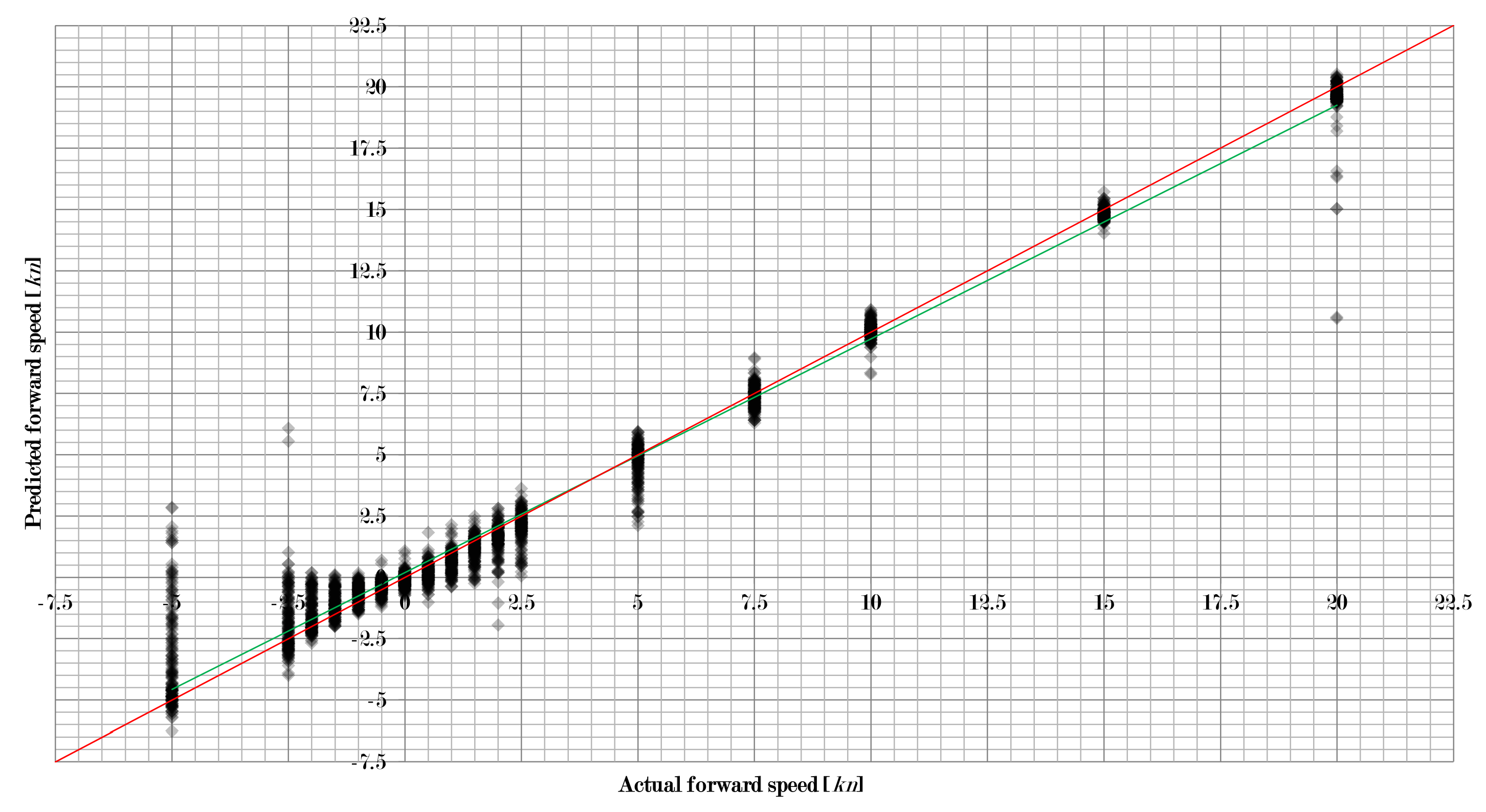
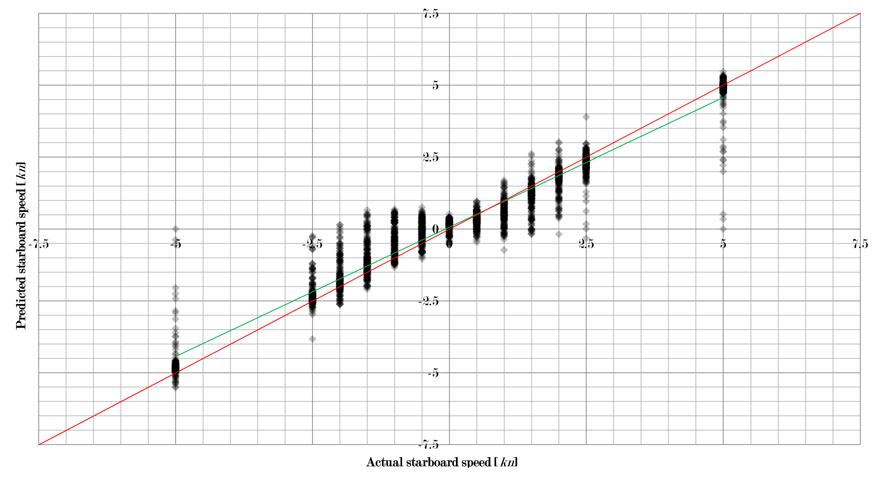
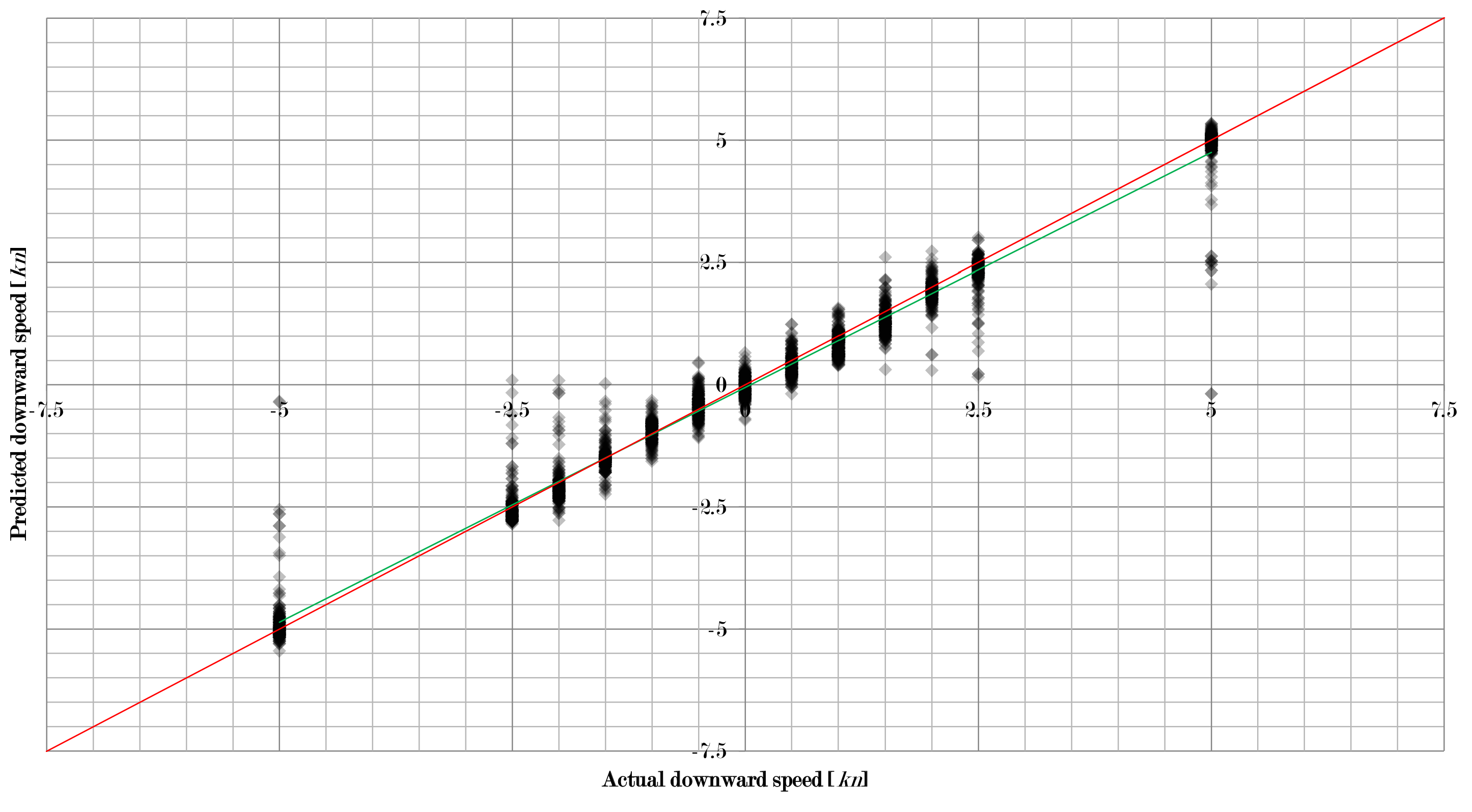
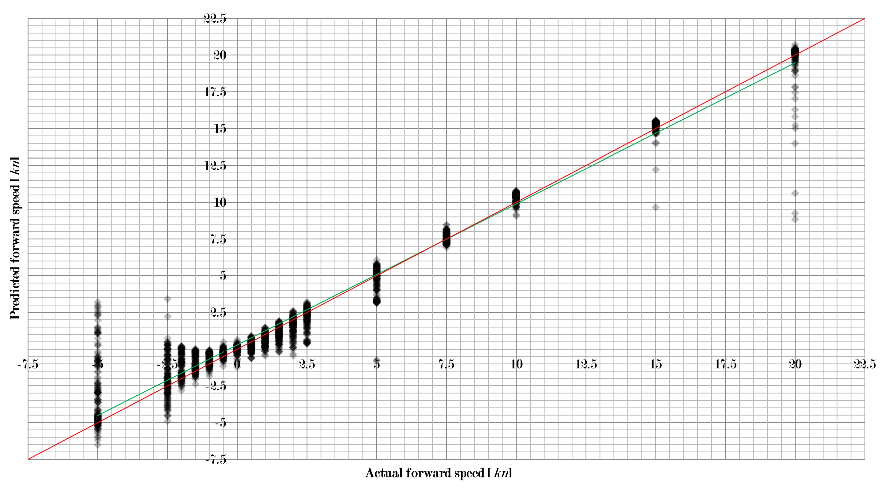
Figure 3,
Figure 4 and
Figure 5 show how the approach in this study worked for the three velocity components separately when using a combination of learning machine and pre-processing with a low RMSE. For all 2873 flow situations, the speed predicted by the algorithm was compared to the actual speed set in the simulation. The intensity of diamonds indicates the number of results. Hence, a black diamond shows that there are many results falling in this area.
As one can see, quite a large number of results are very close to the perfect prediction (red line). However, some results deviate significantly. Thus, there are problems with some unique flow situations that need to be addressed. It can also be observed that the linear fit of the data (green line) is very close to the perfect prediction as well, which indicates that the overall performance is very good.
Figure 3,
Figure 4 and
Figure 5 also show that the absolute error first increased and then decreased with increasing flow velocity. For the forward/backward component of the velocity, the peak was at 5 kn, for the sidewards motion it was at 2 kn, and for the upward/downward component the peak was at 1.5 kn. This results in the relative error decreasing with increasing velocity. Hence, low velocities are more difficult to work with than higher velocities. However, higher velocities also produce more outliers.
5. Optimising the Position of Pressure Measurement Points
5.1. Optimisation
During the numerical simulations, it could be observed that the changes in pressure near the pressure measurement points are not the most significant ones over the whole surface of the AUV’s body. Other regions are more strongly influenced by the changes in velocity. It is sensible to assume that, by moving the pressure measurement points to regions with higher pressure variations, the performance of the learning machines can be increased. Furthermore, a more optimal positioning may allow a smaller number of measurement points, which in turn reduces the complexity of the learning machines.
The following observations can be made about the pressure distribution:
Sideward, upward, and downward flow velocity components resulted in significant pressure changes on the fins. There were distinct high pressure regions on the upstream side and low pressures on the downstream side.
Forward and backward flow velocity components resulted in an increase in pressure near the bow and the stern, respectively.
The isobars on the AUV’s body were parallel and almost horizontal in all flow situations.
For skew angles of attack, the pressure changes were not well-captured, as the most significant changes and the velocity head were in between the lines on which the pressure measurement points are distributed.
These observations led to the following changes in the positioning of the pressure measurement points:
Place measurement points on both sides of each fin to capture the significant pressure changes and especially the differences between the upstream and the downstream sides.
Keep the most forward and most backward pressure measurement points as these are the only points that can capture the changes due to a forward and backward flow velocity component.
It is sufficient to have one set of measurement points on the cylindrical part of the AUV’s body as the points along one line measure almost the same pressure and are therefore redundant.
Introduce additional pressure measurement points in between the lines where the measurement points are currently placed such that the points are not only at the top, the bottom, and the two sides.
Figure 6 shows the resulting positions of the measurement points when the above steps were applied. As one can see, there were now four sets of eight points each, which gives a total of 32 pressure measurement points. The positions of the measurement points were as follows:
For the front, middle, and rear set, the points were equally-spaced at 45 with respect to each other when viewed along the x-axis. The front set was at 500 mm from the bow. The middle set was exactly in the middle of the AUV’s body. The rear set was at 500 mm from the stern. The positions of the points on the fins can be found by the intersection of the two diagonals on each side of every fin.
One may also observe that there were now much fewer than the original 56 points. Hence, a reduction of the number of measurement points was also achieved. This would also give less complex learning machines.
5.2. Results and Discussion
Table 3 shows the root mean square errors (RMSE) for all combinations of the five machine learning methods and the five different input data for the velocity components along the three axes of a Cartesian coordinate system. As it is only an RMSE as before, the actual difference between the velocity obtained from the algorithm and the expected velocity can deviate significantly. The root mean square errors for forward/backward motion were slightly higher while the root mean square errors for upward/downward motion were slightly lower than the values given in the table.
As one can see, k-nearest neighbour showed a large RMSE for raw data input (Raw) and fast Fourier transformed input (FFT) of above 18 kn. Furthermore, no meaningful results could be obtained for the other three input methods. For artificial neural networks, the RMSE was just above 4 kn for all input methods. The RMSE’s for Bayesian networks (BN) were between 3 kn and 4 kn, except with moving averages, where it was a little bit higher. For multiple linear regression (MLR), the root mean square error was around 1.5 kn except with singular value decomposition, where it was above 2 kn. Support vector machines yielded the lowest RSME when using raw data or Fourier transformed data (less than 0.7 kn). With the other input methods, the root mean square error was significantly higher.
When compared to the original results (
Table 2), some notable changes in the errors could be observed. Some of the input data/learning machine combinations showed a significant decrease in performance, while others performed very well. Artificial neural networks did not show very much change. There were some slight increases and decreases in the RMSE depending on the input data. Support vector machines and Bayesian networks all showed a small increase in performance with the exception of BN with SVD where the error was doubled. Multiple linear regression all showed a small decrease in performance with the exception of MLR with SVD where the error was reduced by almost 1 kn. Finally,
k-nearest neighbour, which already showed bad results in the original setting, performed even worse with the new setup.
Multiple linear regression showed good results, although the RMSE was slightly higher than before. This suggests that the pressure/velocity relation in the new setup was again quite linear. As before, pre-processing the pressure data reduced the performance of the learning algorithms. The exception was fast Fourier transformation, which increased the performance slightly in the cases of ANN, KNN, and SVM.
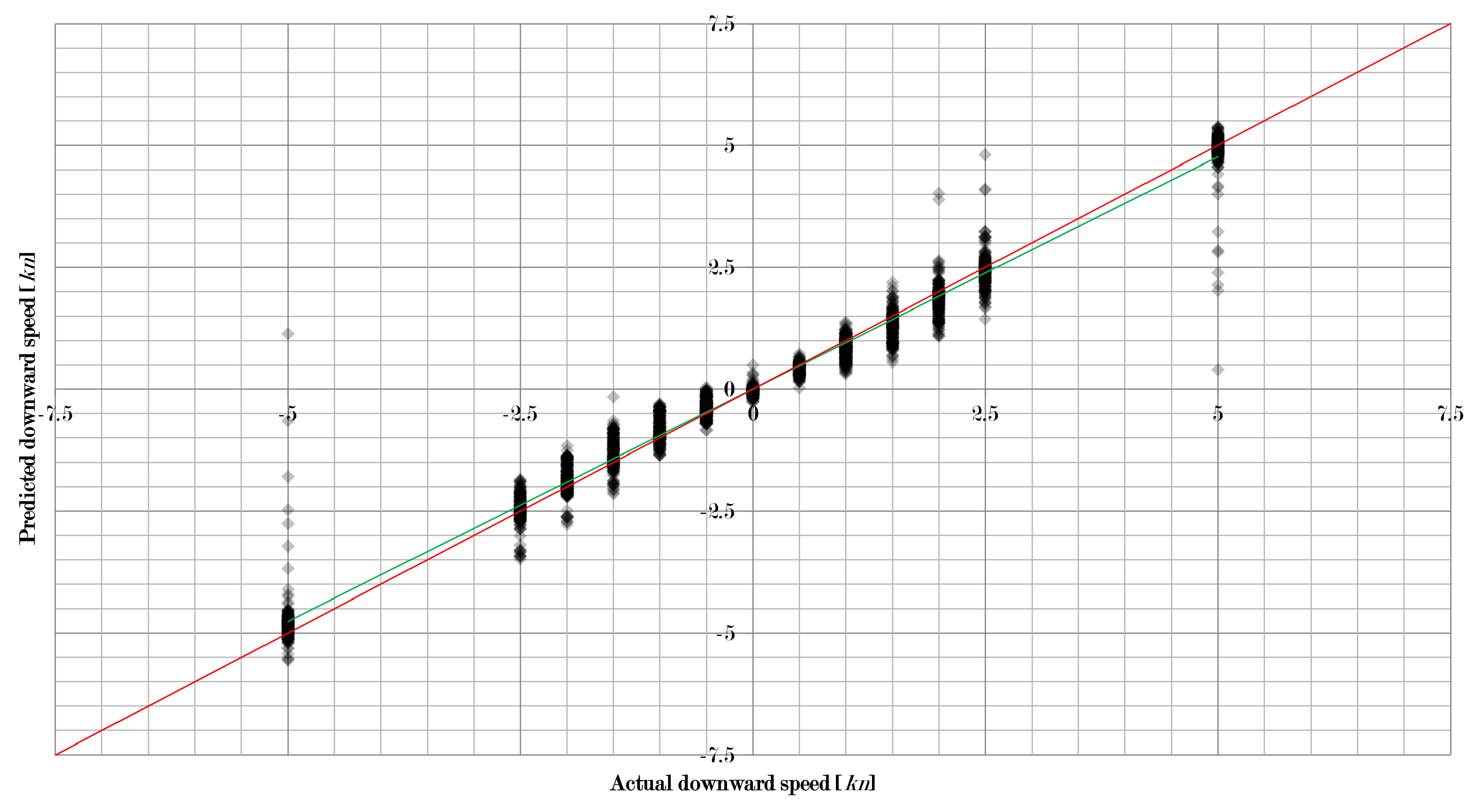
Figure 7,
Figure 8 and
Figure 9 show how the approach in this study worked for the three velocity components separately when using a combination of learning machine and pre-processing with a low RMSE. For all 2873 flow situations, the speed predicted by the algorithm was compared to the actual speed set in the simulation. The intensity of diamonds indicates the number of results. Hence, a black diamond shows that there are a large number of results falling into this area.
As one can see, quite a large number of results are very close to the perfect prediction (red line). However, some results deviate significantly. Thus, there are problems with some unique flow situations that need to be addressed. It can also be observed that the linear fit of the data (green line) is very close to the perfect prediction as well, which indicates that the overall performance is very good.
When compared to
Figure 3,
Figure 4 and
Figure 5, one may observe that there are fewer outliers and the other points are much closer to the perfect prediction. The improvement is visualised quite well. However, the remaining outliers are much further out than for the original setup. In addition, the linear fit of the data is much closer to the perfect fit compared to the original setup.
6. Conclusions and Outlook
Within this study, the applicability of different learning methods for determining flow parameters of a surrounding fluid from pressure on an AUV body were tested based on numerous computational fluid dynamical simulations and using pressure data from 56 specified points on the surface of the AUV. These points were situated on four lines along the starboard side, the port side, the top, and the bottom of the AUV body. It was shown that support vector machines are excellent choices to perform this task, provided that the pressure data are pre-processed appropriately. It was also shown that the deviation between the velocity determined by the algorithms and the actual velocity first increases and then decreases with increasing velocity.
With the findings from the simulations, the position of pressure measurement points were then optimised so that the most significant pressure changes due to changing flow velocities could be captured. The measurement points were then situated on three rings, one near the nose, one in the middle section, one near the stern, and on the top and bottom of each fin of the AUV. Each set contained eight points. This reduced the number of measurement points to 32. It was then shown that, for the optimised setup support, vector machines were also the best choices for the given task. However, the machines were less complex in this case due to fewer inputs.
The approach presented currently uses the original pressure data without any additional filtering except for the removal of frequency noise via fast Fourier transform. In the next step, pre-filters should be included into the algorithm to remove unwanted influences due to outliers, measurement errors, and noise, and hence make the algorithm more robust. The influence of the propellers should also be taken into account. It was neglected in this study.
Furthermore, the accuracy of the approach should be improved for small velocities. This is of particular interest since AUVs executing SLAM are usually quite slow (only a few knots). At these flow velocities, fluctuations need to be considered. The reason is that, although the fluctuations are smaller for lower velocities, they become large relative to the flow velocity and therefore have a significant influence on the results. In this approach, Reynolds-averaged Navier–Stokes equations (RANS) were used, which are not good at capturing these fluctuations. Hence, in the next step, the near-wall regions need to be resolved and analysed in detail with respect to the fluctuation of the surface pressure due to the water flow and the surface roughness.
In addition, the approach presented currently does not work for a stationary solution where the fluid is moving but the relative velocity between the AUV and the fluid is zero. To be able to capture this situation, a new type of “active pressure and shear stress sensor”, which is small and lightweight is currently under development.
Finally, it is planned to carry out several experiments with a real AUV body. This will enable the evaluation of the method and its applicability in real situations. In addition, the experiments will result in a significantly higher number of datasets than obtained in this study with CFD, which in turn will allow for further improvement of the approach.
Author Contributions
Conceptualisation, J.H. and W.K.; methodology, J.H.; software, J.H. and W.K.; validation, J.H. and W.K.; formal analysis, J.H. and W.K.; investigation, J.H.; resources, W.K.; data curation, J.H.; writing—original draft preparation, J.H.; writing—review and editing, W.K.; visualisation, J.H.; supervision, W.K.; project administration, J.H.; and funding acquisition, W.K.
Funding
This research received no external funding.
Acknowledgments
The authors would like to thank Johannes Gottschling from the Chair of Mathematics for Engineers at the University of Duisburg-Essen for his insights into statistical learning.
Conflicts of Interest
The authors declare no conflict of interest.
Abbreviations
The following abbreviations are used in this manuscript:
| ADCP | Acoustic Doppler Current Profiler |
| ANN | Artificial Neural Network |
| AUV | Autonomous Underwater Vehicle |
| BN | Bayesian Network |
| CFD | Computational Fluid Dynamics |
| Conv | Convolution |
| DPS | Differential Pressure Sensors |
| EKF | Extended Kalman Filter |
| FFT | Fast Fourier Transform |
| IMU | Inertial Measurement Unit |
| KNN | k-Nearest Neighbour |
| MA | Moving Average |
| MLR | Multiple Linear Regression |
| RANS | Reynolds-Averaged Navier-Stokes equations |
| RSME | Root Mean Square Error |
| SLAM | Simultaneous Localisation and Mapping |
| SVD | Singular Value Decomposition |
| SVM | Support Vector Machine |
| UKF | Unscented Kalman Filter |
| UUV | Unmanned Undersea Vehicle |
References
- Chance, T.S.; Northcutt, J. Deep Water AUV Experience; C & C Technologies: Bridgewater, NJ, USA, 2001. [Google Scholar]
- Wynna, R.B.; Huvennea, V.A.I.; Basa, T.P.L.; Murtona, B.J.; Connellya, D.P.; Betta, B.J.; Ruhla, H.A.; Morrisa, K.J.; Peakallb, J.; Parsonsc, D.R.; et al. Autonomous Underwater Vehicles (AUVs): Their past, present and future contributions to the advancement of marine geoscience. Mar. Geol. 2014, 352, 451–468. [Google Scholar] [CrossRef]
- Bingham, B. Navigating Autonomous Underwater Vehicles. In Underwater Vehicles; Inzartsev, A., Ed.; IntechOpen: London, UK, 2009; pp. 33–50. ISBN 978-9537619497. [Google Scholar]
- Mueller, D.S.; Wagner, C.R.; Rehmel, M.S.; Oberg, K.A.; Rainville, F. Measuring discharge with acoustic Doppler current profilers from a moving boat. In U.S. Geological Survey Techniques and Methods, Book 3; U.S. Geological Survey: Reston, VA, USA, 2013; ISSN 2328-7047. [Google Scholar]
- Paull, L.; Saeedi, S.; Seto, M.; Li, H. AUV Navigation and Localization: A Review. IEEE J. Ocean. Eng. 2014, 39, 131–149. [Google Scholar] [CrossRef]
- Wendel, J. Integrierte Navigationssysteme—Sensordatenfusion, GPS und Inertiale Navigation; De Gruyter Oldenbourg: Berlin, Germany, 2011; ISBN 978-3486704396. [Google Scholar]
- Klein Associates. Available online: http://www.l-3mps.com/Klein/ (accessed on 31 May 2016).
- Shang, Z.; Ma, X.; Liu, Y.; Yan, S. Attitude Determination of Autonomous Underwater Vehicles based on Pressure Sensor Array. In Proceedings of the 2015 CCC, Hangzhou, China, 28–30 July 2015. [Google Scholar] [CrossRef]
- Fan, Z.; Chen, J.; Zou, J.; Li, J.; Liu, C.; Delcomyn, F. Development of artificial lateral-line flow sensors. In Proceedings of the Solid-State Sensor, Actuator and Microsystem Workshop, Hilton Head Island, SC, USA, 2–6 June 2002. [Google Scholar]
- Martiny, N.; Sosnowski, S.; Kühnlenz, K.; Hirche, S.; Nie, Y.; Franosch, J.-M.P.; van Hemmen, J.L. Design of a Lateral-Line Sensor for an Autonomous Underwater Vehicle. In Proceedings of the 2009 IFAC International Conference on Manoeuvring and Control of Marine Craft, Guarujá, Brazil, 16–18 September 2009. [Google Scholar] [CrossRef]
- Muhammad, N.; Strokina, N.; Toming, G.; Tuhtan, J.; Kämäräinen, J.-K.; Kruusmaa, M. Flow feature extraction for underwater robot localization: Preliminary results. In Proceedings of the 2015 IEEE ICRA, Seattle, WA, USA, 26–30 May 2015. [Google Scholar] [CrossRef]
- Yen, W.-K.; Sierra, D.M.; Guo, J. Controlling a Robotic Fish to Swim Along a Wall Using Hydrodynamic Pressure Feedback. IEEE J. Ocean. Eng. 2018, 43, 369–380. [Google Scholar] [CrossRef]
- Xu, Y.; Mohseni, K. A Pressure Sensory System Inspired by the Fish Lateral Line: Hydrodynamic Force Estimation and Wall Detection. IEEE J. Ocean. Eng. 2017, 42, 532–543. [Google Scholar] [CrossRef]
- Asadnia, M.; Kooapalli, A.G.P.; Shen, Z.; Miao, J.M.; Barbastathis, G.; Triantafyllou, M.S. Flexible, zero powered, piezoelectric MEMS pressure sensor arrays for fish-like passive underwater sensing in marine vehicles. In Proceedings of the IEEE MEMS 2013, Taipei, Taiwan, 20–24 January 2013. [Google Scholar] [CrossRef]
- Kooapalli, A.G.P.; Asadnia, M.; Shen, Z.; Miao, J.M.; Tan, C.W.; Barbastathis, G.; Triantafyllou, M. Polymer MEMS pressure sensor arrays for fish-like underwater sensing applications. Micro Nano Lett. 2012, 7, 1189–1192. [Google Scholar] [CrossRef]
- Antonelli, G. Underwater Robots; Springer: Heidelberg, Germany, 2006; ISBN 978-3319028767. [Google Scholar]
- Whitcomb, L.L.; Yoerger, D.R.; Singh, H. Combined Doppler/LBL based navigation of underwater vehicles. In Proceedings of the 11th International Symposium on Unmanned Untethered Submersible Technology, Durham, UK, 22–25 August 1999. [Google Scholar]
- Suzuki, H.; Sakaguchi, J.; Inoue, T.; Watanabe, Y.; Yoshida, H. Evaluation of methods to Estimate Hydrodynamic Force Coefficients of Underwater Vehicle based on CFD. IFAC Proc. Vol. 2013, 46, 197–202. [Google Scholar] [CrossRef]
- Li, M.; Shang, Z.; Wang, R.; Li, T. Attitude Determination of Autonomous Underwater Vehicles based on Hydrodynamics. In Proceedings of the 2016 WCICA, Guilin, China, 12–15 June 2016. [Google Scholar] [CrossRef]
- Bayat, M.; Crasta, N.; Aguiar, A.P.; Pascoal, A.M. Range-Based Underwater Vehicle Localization in the Presence of Unknown Ocean Currents: Theory and Experiments. IEEE Trans. Control Syst. Technol. 2016, 24, 122–139. [Google Scholar] [CrossRef]
- Williams, D.P.; Baralli, F.; Micheli, M.; Vasoli, S. Adaptive underwater sonar surveys in the presence of strong currents. In Proceedings of the 2016 IEEE ICRA, Stockholm, Sweden, 16–21 May 2016. [Google Scholar] [CrossRef]
- Osborn, J.; Qualls, S.; Canning, J.; Anderson, M.; Edwards, D.; Wolbrecht, E. AUV State Estimation and Navigation to Compensate for Ocean Currents. In Proceedings of the MTS/IEEE OCEANS 2015, Washington, DC, USA, 19–22 October 2015. [Google Scholar] [CrossRef]
- Allotta, B.; Costanzi, R.; Fanelli, F.; Monni, N.; Paolucci, L.; Ridolfi, A. Sea currents estimation during AUV navigation using Unscented Kalman Filter. IFAC PapersOnLine 2017, 50, 13668–13673. [Google Scholar] [CrossRef]
- Gao, A.; Triantafyllou, M. Bio-inspired pressure sensing for active yaw control of underwater vehicles. In Proceedings of the IEEE OCEANS 2012, Hampton Roads, VA, USA, 14–19 October 2012. [Google Scholar] [CrossRef]
- Fuentes-Pérez, J.F.; Kalev, K.; Tuhtan, J.A.; Kruusmaa, M. Underwater vehicle speedometry using differential pressure sensors: Preliminary results. In Proceedings of the 2016 IEEE/OES AUV, Tokyo, Japan, 6–9 November 2016. [Google Scholar] [CrossRef]
- Fuentes-Pérez, J.F.; Meurer, C.; Tuhtan, J.A.; Kruusmaa, M. Differential Pressure Sensors for Underwater Speedometry in Variable Velocity and Acceleration Conditions. IEEE J. Ocean. Eng. 2018, 43, 418–426. [Google Scholar] [CrossRef]
- Aleksander, I.; Morton, H. An Introduction to Neural Computing, 2nd ed.; Cengage Learning EMEA: Andover, UK, 1995; ISBN 978-1850321675. [Google Scholar]
- McCulloch, W.; Pitts, W. A logical calculus of the ideas immanent in nervous activity. Bull. Math. Biophys. 1943, 5, 115–133. [Google Scholar] [CrossRef]
- Kim, Y.-S.; Seok, S.; Lee, J.-S.; Lee, S.K.; Kim, J.-G. Optimizing anode location in impressed current cathodic protection system to minimize underwater electric field using multiple linear regression analysis and artificial neural network methods. Eng. Anal. Bound. Elem. 2018, 96, 84–93. [Google Scholar] [CrossRef]
- Lu, H.; Li, Y.; Uemura, T.; Kim, H.; Serikawa, S. Low illumination underwater light field images reconstruction using deep convolutional neural networks. Future Gener. Comput. Syst. 2018, 82, 142–148. [Google Scholar] [CrossRef]
- Wang, X.; Jiao, J.; Yin, J.; Zhao, W.; Han, X.; Sun, B. Underwater sonar image classification using adaptive weights convolutional neural network. Appl. Acoust. 2019, 146, 145–154. [Google Scholar] [CrossRef]
- Chame, H.F.; Machado dos Santos, M.; Silvia, S.d.C.B. Neural network for black-box fusion of underwater robot localization under unmodeled noise. Robot. Auton. Syst. 2018, 110, 57–72. [Google Scholar] [CrossRef]
- Elhaki, O.; Shojaei, K. Neural network-based target tracking control of underactuated autonomous underwater vehicles with a prescribed performance. Ocean Eng. 2018, 167, 239–256. [Google Scholar] [CrossRef]
- Ferreira, C. Designing Neural Networks Using Gene Expression Programming. In Applied Soft Computing Technologies: The Challenge of Complexity; Abraham, A., Köppen, M., Nickolay, B., Eds.; Springer: Heidelberg, Germany, 2006; pp. 517–535. ISBN 978-3540316497. [Google Scholar]
- Haykin, S. Neural Networks and Learning Machines; Pearson Education: London, UK, 2009; ISBN 978-0131293762. [Google Scholar]
- Rojas, R. Neural Networks: A Systematic Introduction; Springer: Heidelberg, Germany, 1996; ISBN 978-3540605058. [Google Scholar]
- Bablani, A.; Edla, D.R.; Dodi, S. Classification of EEG Data using k-Nearest Neighbor approach for Concealed Information Test. Procedia Comput. Sci. 2018, 143, 242–249. [Google Scholar] [CrossRef]
- Guo, Y.; Han, S.; Li, Y.; Zhanga, X.; Bai, Y. k-Nearest Neighbor combined with guided filter for hyperspectral image classification. Procedia Comput. Sci. 2018, 129, 159–165. [Google Scholar] [CrossRef]
- Müller, P.; Salminen, K.; Nieminen, V.; Kontunen, A.; Karjalainen, M.; Isokoski, P.; Rantala, J.; Savia, M.; Väliaho, J.; Kallio, P.; et al. Scene classification by K nearest neighbors using ion-mobility spectrometry measurements. Expert Syst. Appl. 2019, 115, 593–606. [Google Scholar] [CrossRef]
- Fix, E.; Hodges, J.L. Discriminatory analysis, nonparametric discrimination: Consistency properties. Int. Stat. Rev. Revue Int. Stat. 1989, 57, 238–247. [Google Scholar] [CrossRef]
- Lewicki, P.; Hill, T. Statistics: Methods and Applications; StatSoft: Tulsa, OK, USA, 2005. [Google Scholar]
- Drucker, H.; Burges, J.C.; Kaufman, L.; Smola, A.; Vapnik, V. Support Vector Regression Machines. In Advances in Neural Information Processing Systems 9; Mozer, M.C., Jordan, M.I., Petsche, T., Eds.; MIT Press: Cambridge, MA, USA, 1997; pp. 155–161. [Google Scholar]
- Cortes, C.; Vapnik, V. Support-Vector Networks. Mach. Learn. 1995, 20, 273–297. [Google Scholar] [CrossRef]
- Richhariya, B.; Tanveer, M. EEG signal classification using universum support vector machine. Expert Syst. Appl. 2018, 106, 169–182. [Google Scholar] [CrossRef]
- Huang, S.; Cai, N.; Pacheco, P.P.; Narandes, S.; Wang, Y.; Xu, W. Applications of Support Vector Machine (SVM) Learning in Cancer Genomics. Cancer Genom. Proteom. 2018, 15, 41–51. [Google Scholar] [CrossRef]
- Morales, N.; Toledo, J.; Acosta, L. Path planning using a Multiclass Support Vector Machine. Appl. Soft Comput. 2016, 43, 498–509. [Google Scholar] [CrossRef]
- Qiao, X.; Bao, J.; Zhang, H.; Wana, F.; Li, D. Underwater sea cucumber identification based on Principal Component Analysis and Support Vector Machine. Measurement 2019, 133, 444–455. [Google Scholar] [CrossRef]
- Schölkopf, B. Support Vector Learning. Ph.D. Thesis, Technische Universität, Berlin, Germany, 1997. [Google Scholar]
- Press, W.H.; Teukolsky, S.A.; Vetterling, W.T.; Flannery, B.P. Numerical Recipes; Cambridge University Press: Cambridge, UK, 2007; ISBN 978-0521880688. [Google Scholar]
- Jaynes, E.T.; Bretthorst, G.L. Probability Theory: The Logic of Science: Principles and Elementary Applications; Cambridge University Press: Cambridge, UK, 2003; ISBN 978-0521592710. [Google Scholar]
- Ben-Gal, I. Bayesian Networks. In Encyclopedia of Statistics in Quality & Reliability; Ruggeri, F., Kenett, R.S., Faltin, F.W., Eds.; Wiley & Sons: Hoboken, NJ, USA, 2007; ISBN 978-0470018613. [Google Scholar]
- Li, X.; Zhang, L.; Zhang, S. Efficient Bayesian networks for slope safety evaluation with large quantity monitoring information. Geosci. Front. 2018, 9, 1678–1687. [Google Scholar] [CrossRef]
- Naili, M.; Bourahla, M.; Naili, M.; Tari, A.K. Stability-based Dynamic Bayesian Network method for dynamic data mining. Eng. Appl. Artif. Intell. 2019, 77, 283–310. [Google Scholar] [CrossRef]
- Shen, Y.; Zhanga, L.; Zhanga, J.; Yangb, M.; Tangc, B.; Lid, Y.; Leia, K. CBN: Constructing a clinical Bayesian network based on data from the electronic medical record. J. Biomed. Inform. 2018, 88, 1–10. [Google Scholar] [CrossRef]
- Shi, H.; Lin, Z.; Zhang, S.; Li, X.; Hwang, K.-S. An adaptive decision-making method with fuzzy Bayesian reinforcement learning for robot soccer. Inf. Sci. 2018, 436–437, 268–281. [Google Scholar] [CrossRef]
- Brito, M.; Griffiths, G. A Bayesian approach for predicting risk of autonomous underwater vehicle loss during their missions. Reliab. Eng. Syst. Saf. 2016, 146, 55–67. [Google Scholar] [CrossRef]
- Hegde, J.; Utne, I.B.; Schjølberg, I.; Thorkildsen, B. A Bayesian approach to risk modeling of autonomous subsea intervention operations. Reliab. Eng. Syst. Saf. 2018, 175, 142–159. [Google Scholar] [CrossRef]
- Cooper, G.F.; Herskovits, E. A Bayesian method for the induction of probabilistic networks from data. Mach. Learn. 1992, 9, 309–347. [Google Scholar] [CrossRef]
- Heckerman, D.; Geiger, D.; Chickering, D.M. Learning Bayesian networks: The combination of knowledge and statistical data. Mach. Learn. 1995, 20, 197–243. [Google Scholar] [CrossRef]
- Friedman, N.; Geiger, D.; Goldszmidt, M. Bayesian network classifiers. Mach. Learn. 1997, 29, 131–163. [Google Scholar] [CrossRef]
- Gámez, J.A.; Mateo, J.L.; Puerta, J.M. Learning Bayesian networks by hill climbing: Efficient methods based on progressive restriction of the neighborhood. Data Min. Knowl. Discov. 2011, 22, 106–148. [Google Scholar] [CrossRef]
- Lemos, T.; Kalivas, J.H. Leveraging multiple linear regression for wavelength selection. Chemom. Intell. Lab. Syst. 2017, 168, 121–127. [Google Scholar] [CrossRef]
- Kong, Y.S.; Abdullah, S.; Schramm, D.; Omar, M.Z.; Haris, S.M. Development of multiple linear regression-based models for fatigue life evaluation of automotive coil springs. Mech. Syst. Signal Process. 2019, 118, 675–695. [Google Scholar] [CrossRef]
- Ghorbani, M.A.; Asadi, H.; Makarynskyy, O.; Makarynska, D.; Yaseen, Z.M. Augmented chaos-multiple linear regression approach for prediction of wave parameters. Eng. Sci. Technol. Int. J. 2017, 20, 1180–1191. [Google Scholar] [CrossRef]
- Lefort, R.; Real, G.; Drémeau, A. Direct regressions for underwater acoustic source localization in fluctuating oceans. Appl. Acoust. 2017, 16, 303–310. [Google Scholar] [CrossRef]
- The International Association for the Properties of Water and Steam. Release on the IAPWS Formulation 2008 for the Thermodynamic Properties of Seawater; The International Association for the Properties of Water and Steam: Berlin, Germany, 2008. [Google Scholar]
- Milleroa, F.J.; Feistel, R.; Wright, D.G.; McDougall, T.J. The composition of Standard Seawater and the definition of the Reference-Composition Salinity Scale. Deep-Sea Res. I 2008, 55, 50–72. [Google Scholar] [CrossRef]
- Bardina, J.E.; Huang, P.G.; Coakley, T.J. Turbulence Modeling Validation, Testing, and Development; NASA Ames Research Center: Moffett Field, CA, USA, 1997; No. 110446.
- Launder, B.E.; Spalding, D.B. The numerical computation of turbulent flows. Comput. Method Appl. Mech. 1974, 3, 269–289. [Google Scholar] [CrossRef]
- Ferziger, J.H.; Peric, M. Numerische Strömungsmechanik; Springer: Heidelberg, Germany, 2008; ISBN 978-3540675860. [Google Scholar]
© 2019 by the authors. Licensee MDPI, Basel, Switzerland. This article is an open access article distributed under the terms and conditions of the Creative Commons Attribution (CC BY) license (http://creativecommons.org/licenses/by/4.0/).


