Nominal Stiffness of GT-2 Rubber-Fiberglass Timing Belts for Dynamic System Modeling and Design


Abstract
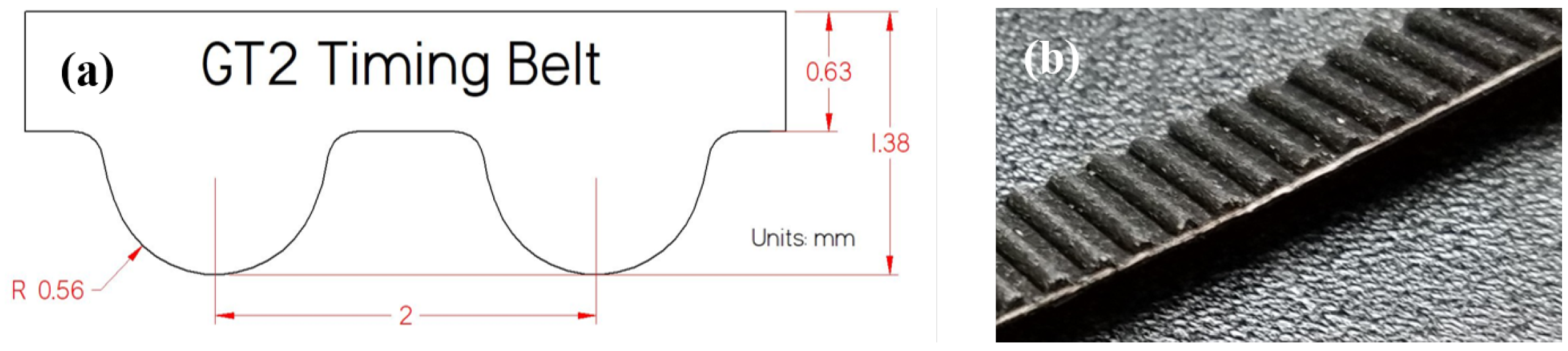
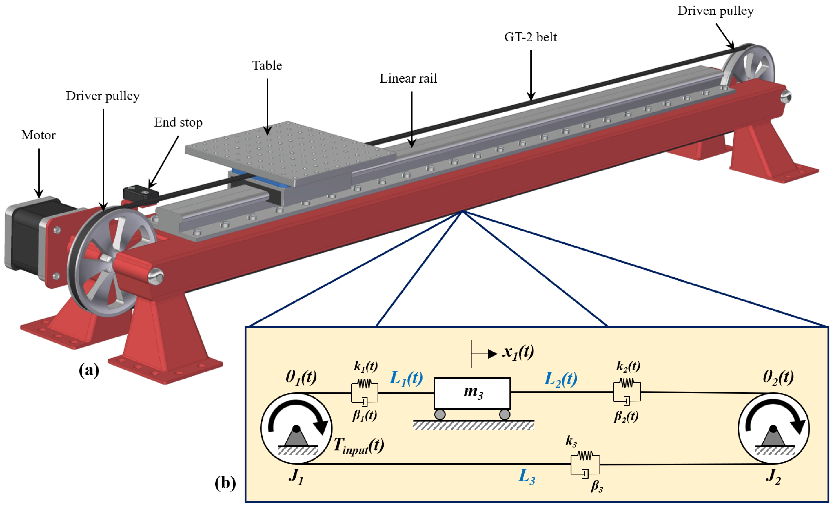
1. Introduction
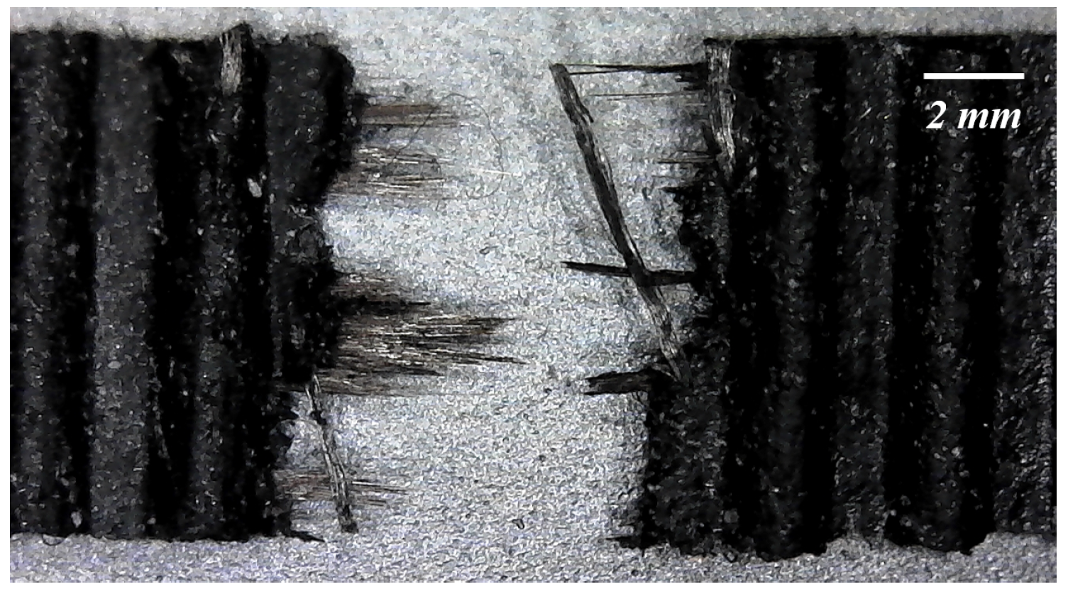
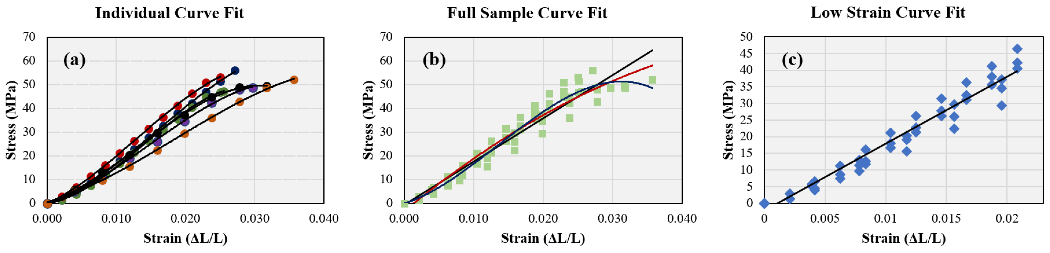
2. Procedure and Results
3. Recommendations for Use and Applications
- Identify the nominal stiffness of each belt type used in the system (e.g., if two thicknesses of belts are used, two different nominal stiffnesses will be present). This information may be collected from manufacturer datasheets or from tests on each belt type, similar to the tests done in this technical report.
- Decide if a linear or nonlinear nominal stiffness model will be used for each belt type. The primary driving force for this decision will be the computational cost for analyzing the system; for a simple system, it may be practical to use a nonlinear nominal stiffness model, but a linear model would be more feasible in a system with several elements. However, the importance of the model accuracy is a serious consideration and may justify a high computational cost if high accuracy is required.
- Based on the configuration of the system and the decisions made in the first two steps, the effective stiffness k can take one of four forms:
- (a)
- If the belt length is constant and a linear model is used for , the effective stiffness in the equations of motion will be constant and described by
- (b)
- If the belt length is constant and a nonlinear model is used to find , the nominal stiffness will be a function derived form a force-deflection curve. The effective stiffness in that belt section will be described bywhere is a continuous function of x.
- (c)
- If the belt length is time-variant and a linear model is used for , the effective stiffness in the equations of motion will be time-variant and described by
- (d)
- If the belt length is time-variant and a nonlinear model is used to find , the nominal stiffness will be a function derived form a force-deflection curve. In this case, the effective belt section stiffness will be described bywhere is a continuous function of x and the belt length is a function of time. Therefore, the effective stiffness will be dependent on both the length of the belt and the amount of force placed on the belt.
4. Conclusions
Author Contributions
Funding
Conflicts of Interest
Nomenclature
- b = Belt width (m)
- = Belt section i damping coefficient
- = Nominal belt stiffness (N/m)
- = Effective (true) belt section i stiffness (N/m)
- = Belt section i length (m)
- = Mass of block i (kg)
- = Pulley i angle (degrees)
References
- Laureto, J.; Pearce, J. Open Source Multi-Head 3D Printer for Polymer-Metal Composite Component Manufacturing. Technologies 2017, 5, 36. [Google Scholar] [CrossRef]
- Krahn, J.; Liu, Y.; Sadeghi, A.; Menon, C. A tailless timing belt climbing platform utilizing dry adhesives with mushroom caps. Smart Mater. Struct. 2011, 20, 115021. [Google Scholar] [CrossRef]
- Parietti, F.; Chan, K.; Asada, H.H. Bracing the human body with supernumerary Robotic Limbs for physical assistance and load reduction. In Proceedings of the IEEE International Conference on Robotics and Automation (ICRA), Hong Kong, China, 31 May–7 June 2014. [Google Scholar]
- Choudhary, R.; Sambhav; Titus, S.D.; Akshaya, P.; Mathew, J.A.; Balaji, N. CNC PCB milling and wood engraving machine. In Proceedings of the International Conference On Smart Technologies For Smart Nation (SmartTechCon), Bangalore, India, 17–19 August 2017. [Google Scholar] [CrossRef]
- Sollmann, K.; Jouaneh, M.; Lavender, D. Dynamic Modeling of a Two-Axis, Parallel, H-Frame-Type XY Positioning System. IEEE/ASME Trans. Mechatron. 2010, 15, 280–290. [Google Scholar] [CrossRef]
- York Industries. York Timing Belt Catalog: 2mm GT2 Pitch (pp. 16). Available online: http://www.york-ind.com/print_cat/york_2mmGT2.pdf (accessed on 13 June 2018).
- SDP/SI. Handbook of Timing Belts, Pulleys, Chains, and Sprockets. Available online: www.sdp-si.com/PDFS/Technical-Section-Timing.pdf (accessed on 13 June 2018).
- Huang, J.L.; Clement, R.; Sun, Z.H.; Wang, J.Z.; Zhang, W.J. Global stiffness and natural frequency analysis of distributed compliant mechanisms with embedded actuators with a general-purpose finite element system. Int. J. Adv. Manuf. Technol. 2012, 65, 1111–1124. [Google Scholar] [CrossRef]
- Barker, C.R.; Oliver, L.R.; Breig, W.F. Dynamic Analysis of Belt Drive Tension Forces During Rapid Engine Acceleration; SAE Technical Paper Series; SAE International: Warrendale, PA, USA, 1991. [Google Scholar]
- Gates-Mectrol. Technical Manual: Timing Belt Theory. Available online: http://www.gatesmectrol.com/mectrol/downloads/download_common.cfm?file=Belt_Theory06sm.pdf&folder=brochure (accessed on 13 June 2018).
- Hace, A.; Jezernik, K.; Sabanovic, A. SMC With Disturbance Observer for a Linear Belt Drive. IEEE Trans. Ind. Electron. 2007, 54, 3402–3412. [Google Scholar] [CrossRef]
- Johannesson, T.; Distner, M. Dynamic Loading of Synchronous Belts. J. Mech. Des. 2002, 124, 79. [Google Scholar] [CrossRef]
- Childs, T.H.C.; Dalgarno, K.W.; Hojjati, M.H.; Tutt, M.J.; Day, A.J. The meshing of timing belt teeth in pulley grooves. Proc. Inst. Mech. Eng. D 1997, 211, 205–218. [Google Scholar] [CrossRef]
- Callegari, M.; Cannella, F.; Ferri, G. Multi-body modelling of timing belt dynamics. Proc. Inst. Mech. Eng. K 2003, 217, 63–75. [Google Scholar] [CrossRef]
- Leamy, M.J.; Wasfy, T.M. Time-accurate finite element modelling of the transient, steady-state, and frequency responses of serpentine and timing belt-drives. Int. J. Veh. Des. 2005, 39, 272. [Google Scholar] [CrossRef]
- Feng, X.; Shangguan, W.B.; Deng, J.; Jing, X.; Ahmed, W. Modelling of the rotational vibrations of the engine front-end accessory drive system: a generic method. Proc. Inst. Mech. Eng. D 2017, 231, 1780–1795. [Google Scholar] [CrossRef]
- Rodriguez, J.; Keribar, R.; Wang, J. A Comprehensive and Efficient Model of Belt-Drive Systems; SAE Technical Paper Series; SAE International: Warrendale, PA, USA, 2010. [Google Scholar]
- Cepon, G.; Boltezar, M. An Advanced Numerical Model for Dynamic Simulations of Automotive Belt-Drives; SAE Technical Paper Series; SAE International: Warrendale, PA, USA, 2010. [Google Scholar]
- Tai, H.M.; Sung, C.K. Effects of Belt Flexural Rigidity on the Transmission Error of a Carriage-driving System. J. Mech. Des. 2000, 122, 213. [Google Scholar] [CrossRef]
- Zhang, L.; Zu, J.W.; Hou, Z. Complex Modal Analysis of Non-Self-Adjoint Hybrid Serpentine Belt Drive Systems. J. Vib. Acoust. 2001, 123, 150. [Google Scholar] [CrossRef]
- Materials Testing Guide; ADMET: Norwood, MA, USA, 2013.
- Kumar, D.; Sarangi, S. Data on the viscoelastic behavior of neoprene rubber. Data Brief. 2018, 21, 943–947. [Google Scholar] [CrossRef] [PubMed]
- Mansouri, M.; Darijani, H. Constitutive modeling of isotropic hyperelastic materials in an exponential framework using a self-contained approach. Int. J. Solids Struct. 2014, 51, 4316–4326. [Google Scholar] [CrossRef]
- Shahzad, M.; Kamran, A.; Siddiqui, M.Z.; Farhan, M. Mechanical Characterization and FE Modelling of a Hyperelastic Material. Mater. Res. 2015, 18, 918–924. [Google Scholar] [CrossRef]
- Tokoro, H. Analysis of transverse vibration in engine timing belt. JSAE Rev. 1997, 18, 33–38. [Google Scholar] [CrossRef]
- Gerbert, G.; Jnsson, H.; Persson, U.; Stensson, G. Load Distribution in Timing Belts. J. Mech. Des. 1978, 100, 208. [Google Scholar] [CrossRef]


| Case | Plot Reference | A | B | C | D | |
|---|---|---|---|---|---|---|
| 760 mm (cubic model) - | Figure 5a | 94,969 | 958.80 | −0.5658 | 0.9996 | |
| 760 mm (cubic model) - | Figure 5a | 144,204 | 445.86 | −0.1163 | 0.9996 | |
| 760 mm (cubic model) - | Figure 5a | 95,693 | 1281.60 | −0.0723 | 0.9997 | |
| 400 mm (cubic model) - | Figure 5a | 81,219 | 849.99 | 0.2296 | 0.9993 | |
| 400 mm (cubic model) - | Figure 5a | 95,332 | 935.37 | 0.2840 | 0.9995 | |
| 400 mm (cubic model) - | Figure 5a | −922,283 | 50,993 | 810.95 | 0.4965 | 0.9994 |
| Full dataset (cubic model) | Figure 5b | 98,091 | 937.22 | −0.1758 | 0.9672 | |
| Full dataset (quadratic model) | Figure 5b | - | −19,340 | 2408.9 | −3.3656 | 0.9552 |
| Full dataset (linear model) | Figure 5b | - | - | 1821.1 | −0.6140 | 0.9431 |
| Low strain (linear model) | Figure 5c | - | - | 2013.8 | −2.3275 | 0.9573 |
© 2018 by the authors. Licensee MDPI, Basel, Switzerland. This article is an open access article distributed under the terms and conditions of the Creative Commons Attribution (CC BY) license (http://creativecommons.org/licenses/by/4.0/).
Share and Cite
Wang, B.; Si, Y.; Chadha, C.; Allison, J.T.; Patterson, A.E. Nominal Stiffness of GT-2 Rubber-Fiberglass Timing Belts for Dynamic System Modeling and Design. Robotics 2018, 7, 75. https://doi.org/10.3390/robotics7040075
Wang B, Si Y, Chadha C, Allison JT, Patterson AE. Nominal Stiffness of GT-2 Rubber-Fiberglass Timing Belts for Dynamic System Modeling and Design. Robotics. 2018; 7(4):75. https://doi.org/10.3390/robotics7040075
Chicago/Turabian StyleWang, Bozun, Yefei Si, Charul Chadha, James T. Allison, and Albert E. Patterson. 2018. "Nominal Stiffness of GT-2 Rubber-Fiberglass Timing Belts for Dynamic System Modeling and Design" Robotics 7, no. 4: 75. https://doi.org/10.3390/robotics7040075
APA StyleWang, B., Si, Y., Chadha, C., Allison, J. T., & Patterson, A. E. (2018). Nominal Stiffness of GT-2 Rubber-Fiberglass Timing Belts for Dynamic System Modeling and Design. Robotics, 7(4), 75. https://doi.org/10.3390/robotics7040075