Abstract
This paper presents a theory for the analytical determination of internal forces in the links of planar linkage mechanisms and manipulators with statically determinate structures, considering the distributed dynamic loads. Linkage mechanisms and manipulators were divided into elements and joints. Discrete models were created for both the elements and the entire mechanism. The dynamic equations of equilibrium for the discrete model of the elements and the hinged and rigid joints, under the action of longitudinal and transverse distributed dynamic trapezoidal loads, were derived. In the dynamic equations of the equilibrium of the discrete model of the elements and joints, the connections between the components of the force vector in the calculated cross-sections and the geometric, physical, and kinematic characteristics of the element were established for its plane-parallel motion. According to the developed technique, programs were created in the Maple system, and animations of the motion of the mechanisms were produced. The links were constructed with the intensity of transverse- and longitudinal-distributed dynamic loads, bending moments, and shearing and normal forces, depending on the kinematic characteristics of the links.
1. Introduction
One of the important problems in designing mechanisms and manipulators is ensuring the strength and stiffness of their links during full-time process. For strength and stiffness analysis, the laws of distribution of internal forces, which enable selecting the form of cross-sections and defining their linear sizes, should be considered.
To analyze the stress–strain state of linkage systems, there are different approaches: graphically analytic methods, forces methods, and displacement methods [1,2,3]. When calculating using the forces method, the main sought-after values are the forces in redundant constraints. Knowledge of the forces in redundant constraints enables the use of sectioning to perform complete calculations to determine the forces that arise in cross-sections of elements in a given system. When calculating using the displacement method, the main sought-after values are the displacements of the nodal points caused by deformation of the system. Knowledge of these displacements is necessary and sufficient to determine all internal forces that arise in cross-sections of elements in the system.
As all linkage systems have distributed mass, they are always systems with a degree of freedom of equal infinity; however, in many cases, it is possible to minimize the calculation of such systems to a calculation with an ultimate number of, or even with one, degree of freedom. One such approach to solve the problem of dynamic calculation of elastic systems is the lumped parameters method. Replacing the distributed masses by concentrated masses is based on the idea of approximate replacement of the system, replacing infinite degrees of freedom in the system with ultimate degrees. Considerable research has been devoted to the lumped parameters method [4,5,6,7,8].
One of the numerical methods that enable the computation of the stress–strain state of linkage systems is the finite element method. In finite element calculation, the system is split into simple finite elements. The matrix of stiffness of an element and the whole system connection is provided by the displacement of joints of the element and the system, as well as forces within [9,10,11,12,13,14,15,16,17,18,19]. Li and Hao [20] proposed a constraint force-based (CFB) modelling approach to model compliant mechanisms with a particular emphasis on modelling complex compliant mechanisms. The proposed CFB modelling approach can be regarded as an improved free-body-diagram (FBD) modelling approach, and was extended to the development of the screw-theory-based design approach.
However, in these graphically analytic and numerical methods for strength and stiffness, the analysis of linkage mechanisms and manipulators, the distributed loads from inertial forces, gravitational forces arising from distributed own mass of links, and changing their values and directions from kinematic parameters of mechanism are not considered. These distributed loads play an essential role in investigating the stress–strain state of the links between mechanisms and manipulators. Therefore, firstly, it is necessary to establish the distribution laws of distributed loads, that is, to find dependencies between the distributed loads and with geometric, physical, and kinematic characteristics of links with constant cross-sections in their plane-parallel movement. Thereafter, the approximation matrix of the forces of the elements that define dependence between the vector of forces in any cross-section of an element, and the vector of forces in calculated cross-sections, is determined. On the found approximation matrices of forces, the compliance matrix of the discrete element, which characterizes physical properties of element, is defined.
For the elastic calculation of linkage mechanisms, based on D’Alambert’s principle, the structures have a degree of freedom equal to zero. To define the internal forces in links of the computational scheme of the mechanism, the structure is divided into elements, as well as hinge and rigid joints. The elements are divided into three types of beams. The discrete models of these beams with constant cross-sections under the action of transverse and longitudinal distributed trapezoidal loads are developed. The constructed discrete models of these beams with constant cross-sections allow the determination of a number of independent dynamic equilibrium equations and the components of vector of forces in calculated cross-sections, and the construction of a discrete model of the entire structure.
This work addresses derived dynamic equilibrium equations for the discrete model of a link element with constant cross-sections under the action of transverse and longitudinal inertial trapezoidal loads. The dynamic equilibrium equations of the discrete model of the elements are derived, and connections are established between the components of vector of forces in calculated cross-sections, with geometric, physical, and kinematic characteristics of links with constant cross-sections in their plane-parallel movement. Thereafter, the equilibrium equations of hinge and rigid joints, expressed through required parameters of internal forces when the elements are subjected to the distributed trapezoidal loads, are derived. Connections between the components of the vectors of the forces in the calculated cross-sections of adjacent elements and the external concentrated loads applied to this joint are examined.
By combining the dynamic equilibrium equations of elements and joints into one system, the dynamic equilibrium equations of the entire discrete model of the system are derived. Such a system of equations is sufficient for determining the internal forces in the links of mechanisms and manipulators with statically determinate structures. The vector of the load and the vector of the force in the calculated cross-sections of discrete models of mechanisms are formed from the vector of loads and the vector of forces in the calculated cross-sections of their separate elements. Through this method, computer programs are developed in the Maple system, and animations of movement of mechanism with the construction of links in terms of intensity of transverse and longitudinal inertial loads, bending moments, and shearing and normal forces, which depend on kinematic characteristics of links, were produced.
2. Distributed Dynamic Loads and Approximation Matrix
Let us consider the plane-parallel movement of the link k of the mechanism with constant cross-sections with respect to the fixed coordinate system OXY. The following laws of distribution of transverse and longitudinal inertial loads along the link that arise from the mass of the link are defined [21]:
where:
where is the angle, defining position of link k with respect to the fixed coordinate system OXY; are the angular velocity and angular acceleration of the link k, respectively; and are the components of acceleration of the point (pole) of the link k, are directed along and perpendicular to the axis of the link k, respectively; is the specific weight of material of the link k; is the square of transverse cross-section of the link k; and is the acceleration of gravity.
The found expressions show that the distribution of transverse and longitudinal inertial forces along the axis of the link with constant cross-sections is characterized by a trapezoidal law.
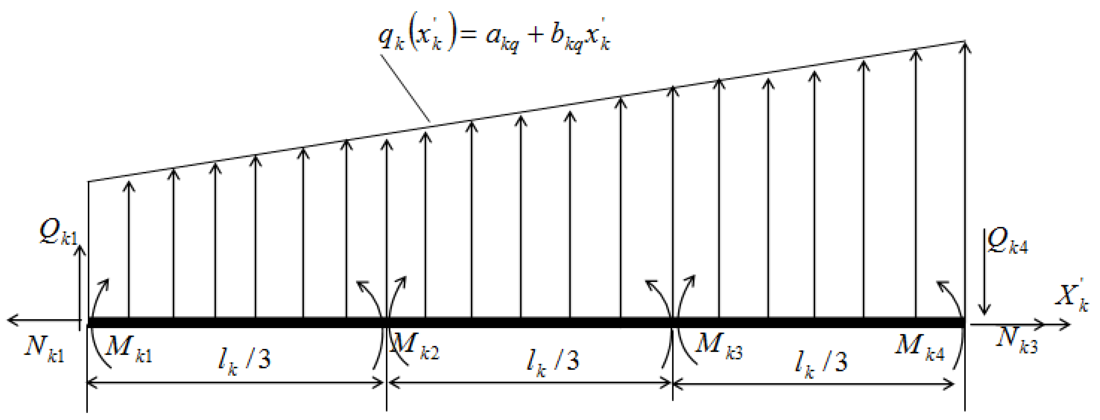
For the element k, which is under the influence of longitudinal distributed trapezoidal loads, as shown in Figure 1, the bending moments along the length of the element are distributed by a law of a third-order polynomial:
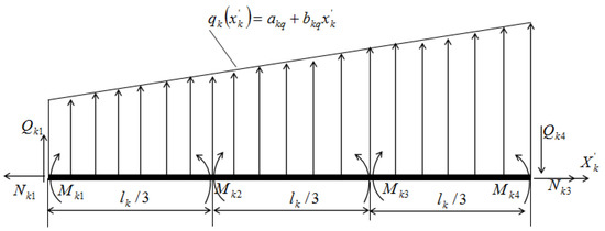
Figure 1.
The element under the action of transverse distributed trapezoidal loads.
Now, express the bending moment in the cross-section through the required bending moments in the cross-sections demonstrated in Figure 1.
For this purpose, it is enough to express the coefficients through , respectively. As a result we have [22]:
Differentiating by results in the equation of the shearing force:
Suppose, in addition to the transverse distributed load, the longitudinal distributed trapezoidal load acts on the element. In this case, the normal force in an arbitrary cross-section of the element can be expressed analogously to the previous expression by means of the normal forces in the calculated cross-sections as follows:
Thus, for the element experiencing transverse and longitudinal distributed trapezoidal loads, the approximation matrix connecting the internal forces in any cross-section of the element, with the values of internal forces in the calculated cross-sections, has the form:
The elements of the first row of this matrix can be seen in Equation (1); the elements of the second row can be seen in Equation (4); and the elements of the third row can be seen in Equation (5).
This expression of the approximation matrix of forces defines the relationship between the vector of forces in any cross-section of the element and the vector of forces in appointed cross-sections . For the element of linkage system, the approximation matrix is found exactly within the framework of the known laws of distribution of unknown forces.
We see that the equations of the bending moment, shearing force and normal forces, in Equations (3)–(5), respectively, which are expressed by the same values in the calculated cross-sections, demonstrate that, to define the internal loads of each element of the mechanism, it is enough to know the values of these loads in a finite number of cross-sections in each of these elements. The number of cross-sections in which it is necessary to know the values of internal forces are defined by the polynomial degrees of external actions. Thus, the internal forces of each continual link are determined unambiguously by a set of internal forces in its separate cross-sections and by the matrices of approximation. Therefore, the task is reduced to calculating internal forces in a finite number of cross-sections of the elements. Hence, we obtain a discrete model of elastic calculation of the links of linkage mechanisms and manipulators.
3. Discrete Models for Elastic Calculation of Elements and Entire Construction of Mechanisms and Manipulators
For elastic calculation of the linkage mechanisms based on D’Alambert’s principle, all distributed dynamic and concentrated loads were attached to the links, as well as unknown driving moments (forces) were attached to the driving links, which ensured the assigned laws of their motion. Therefore, we obtained the construction with degrees of freedom equal to zero, if the rotational kinematic pair that connect the driving link and fixed base are replaced by a rigid restraint.
To define the internal forces in the links (in the elements), the construction of the mechanisms and manipulators was divided into elements and joints. The link or the part of the link could be the element, whereas the joints were the kinematic pairs, connecting the adjacent links and cross-sections where the concentrated external forces were attached.
The process of division of the construction included assignment of the calculated cross-sections of elements and their designations. When dividing the elements of the computational scheme of the construction into calculated cross-sections and joints, it was necessary to establish which internal connections between the elements should remain and which ones should be deleted. After discarding some internal connections or their combinations in the element, the element was then broken up into two elements that can rotate, move, or be removed from each other. To prevent this, the internal forces were attached in place of the discarded connections. Henceforth, these forces were considered the main unknowns [23].
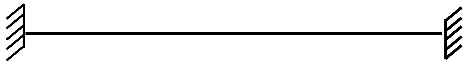
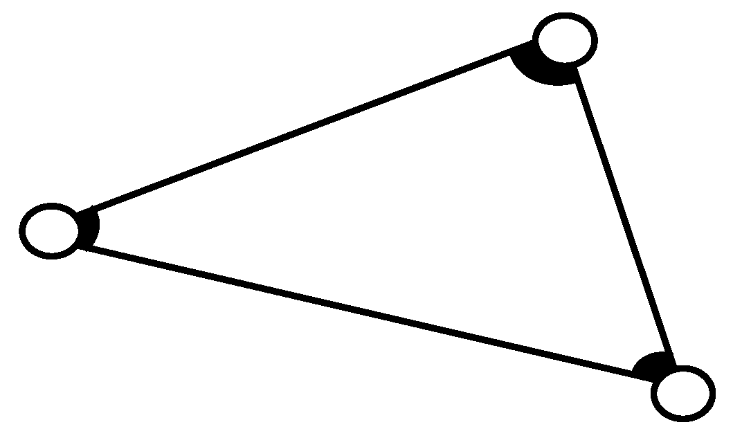
Let us decompose the element of the planar linkage mechanism into three types of beams for the convenience of producing the decisive equations and determining the internal forces in the assigned cross-sections of the elements of mechanism. The first type of the element was a beam with two rigidly fixed ends, as demonstrated in Figure 2. Such beams can be rods with basic links when these rods are interconnected rigidly, as shown in Figure 3.

Figure 2.
The beam in which both ends are connected rigidly (the first type of beam).

Figure 3.
The basic link in which rods are interconnected rigidly.
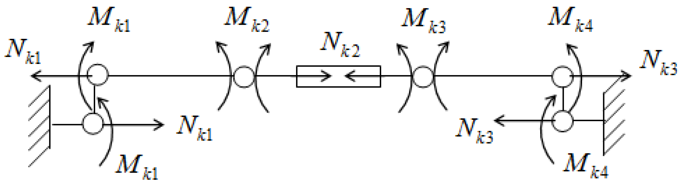
To determine the coefficients of expressions of the bending moment in Equation (3), it was necessary to know the values of the bending moments in the four cross-sections. To determine the coefficients of expressions of the normal forces in Equation (5), it was necessary to know the values of the normal forces in the three cross-sections of the element. Therefore, in this beam, we chose four cross-sections with unknown bending moments and three cross-sections with unknown normal forces. Then, considering the conditional schemes with corresponding unknowns, we constructed the discrete model of the considered beam, shown in Figure 4.
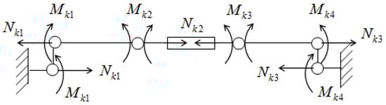
Figure 4.
The discrete model of the first type of beam under the action of distributed trapezoidal loads.
Then, the force vector in the calculated cross-sections of the discrete model for this beam is expressed by the following vector:
There is a dependence between the degree of freedom of discrete model , the number of attached external forces , and the degree of static indeterminacy of the computational scheme [1]:
This equation conveniently simplifies determining the degrees of freedom of the discrete model. The total number of forces in the calculated cross-sections are easily counted, and the degree of static indeterminacy of the computational scheme is found using the formula , where is the number of closed loops, is the number of single hinges, and is the degree of static indeterminacy of computational scheme of mechanism.
The degrees of freedom of the discrete model determines the number of necessary independent equations of statics. Let us define the degrees of freedom of discrete model of this beam. The number of unknowns is , the static indeterminacy of the beam is , so the degrees of freedom of the discrete model In other words, it is possible to derive four independent equilibrium equations for this discrete beam model.
The second type of element is the beam, where one end is fixed rigidly and the other is fixed by the motionless hinge. Such beams can be the driving links of planar linkage mechanisms.
The third type of element is the beam of the intermediate links. They can be considered as beams fixed with motionless hinged supports at both ends. The discrete models for the second and third types of beams can be constructed similarly to the discrete model for the first type of beam.
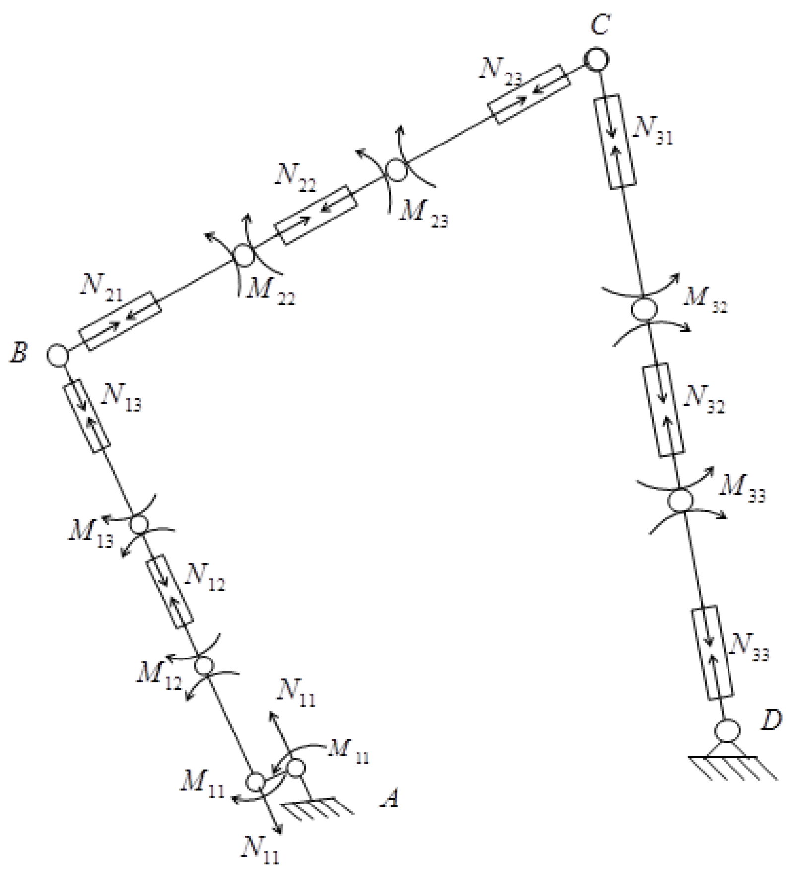
The discrete model of the four-bar linkage is shown in Figure 5, where all the unknown values that define all internal forces in any cross-section of links of the mechanism are illustrated. For the first link (the second type of beam) of this mechanism, the vector of forces in the calculated cross-sections has the following components:

Figure 5.
The discrete model of the four-bar mechanism with constant cross-sections.
For the second and third links (the third type of beam) of the considered mechanism, the vector of the forces in the calculated cross-sections have the following components, respectively:
For the entire discrete model of the mechanism, the vector of the forces in the calculated cross-sections are:
4. Dynamic Equilibrium Equations of the Discrete Models of the Elements and Joints
Let us derive the equations for the dynamic equilibrium of the element. From the applied concentrated external loads and the transverse distributed trapezoidal loads along the axis of the element, the bending moment arises in the arbitrary cross-section and is defined by Equation (2). The bending moment in cross-section of the element that is expressed through the sought-after moments in the calculated cross-sections is determined using Equation (3).
Differentiating Equations (2) and (3) three times by , equating them, and substituting the value of , the first equation of dynamic equilibrium becomes:
The dependence between the values of the sought-after magnitudes of the bending moments in the calculated cross-sections, and the geometric, physical, and kinematic characteristics of the element of the mechanism are found. The second equation of dynamic equilibrium is produced by taking the sum of the moments of all acting forces on the element relative to the center of gravity of the cross-section (Figure 1). Then, the following expression is derived:
where:
This expression is not difficult to derive if we substitute the value into Equation (4).
Substituting the values , and into Equation (13), and summing the coefficients of the same known and unknown magnitudes of the equation into the right-hand side, the second equation of the dynamic equilibrium is produced:
From the longitudinal distributed trapezoidal loads acting on the element, and from the force of the cross-section , normal force occurs in the cross-section of the element, which is defined by:
The normal force in the cross-section of the element, expressed through the normal forces in the calculated cross-sections, is calculated using Equation (5).
Differentiating the Equations (5) and (15) two times by , equating them, and substituting the value of , the third dynamic equilibrium equation is produced:
Projecting all the forces acting on element k onto axle and substituting the values of , the fourth equation of dynamic equilibrium is found:
The resulting system of equations consisting of Equations (12), (14), (16) and (17), can be written down in matrix form:
where:
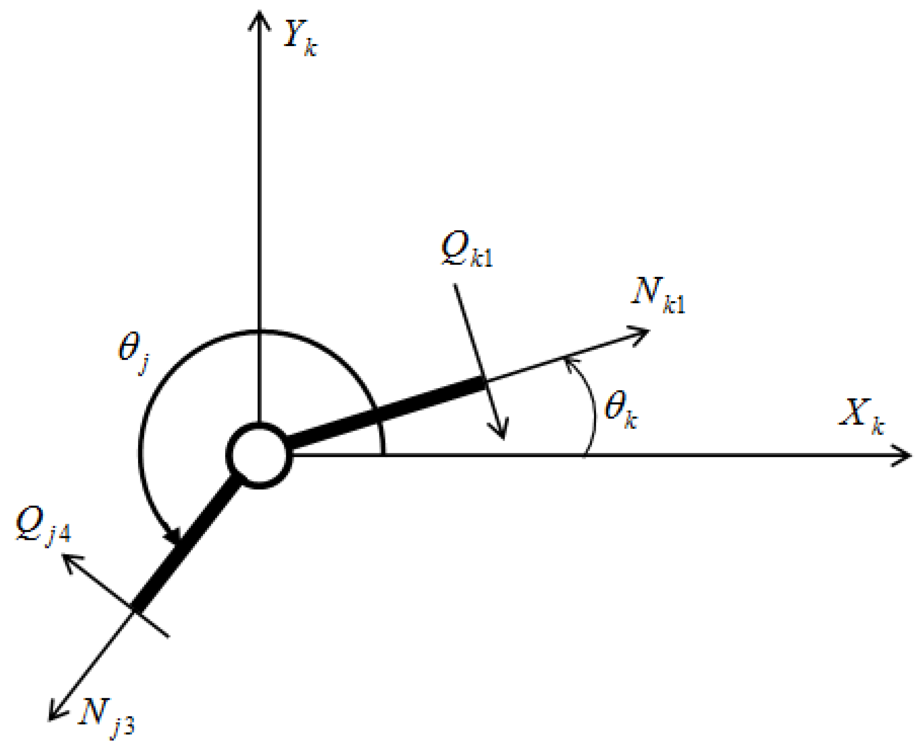
Let the two elements and of the mechanism form a rotational kinematic pair, i.e., tolerate rotational motion relative to each other. Let the length of these elements have constant cross-sections. We cut out the kinematic pair with adjacent cross-sections of the elements forming this pair from the mechanism. In this case, in the cross-sections of the elements adjacent to the joint (to the kinematic pair), the internal forces occur as shown in Figure 6. For such joints, we have two equilibrium conditions. These equilibrium equations for the joint under consideration are written as:
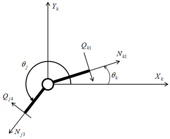
Figure 6.
Hinge joint of the mechanism with constant cross-sections of the element.
The magnitudes of are expressed by means of the sought-after moments in the calculated cross-sections of the discrete model of the elements. To this end, we used Equation (4) for the shearing force, and by substituting the values and , we obtain, respectively:
Now, substituting the values of and into Equation (19), we have the following equilibrium equations for the joint:
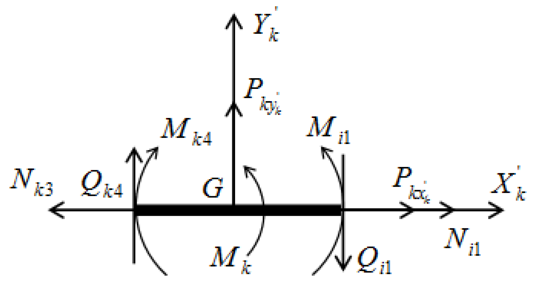
Rigid joints can also be cross-sections of the link where external concentrated forces are applied. The cross-sections of the links can be rigid joints if external concentrated loads are attached in this cross-section. For instance, let the concentrated loads and , and the concentrated moment , be attached to the cross-section of the link (Figure 7). Then, the link is divided into two elements: kth and ith. Figure 7 shows the joint with adjacent cross-sections, where the arising internal forces are shown. For this joint, the following three conditions of dynamic equilibrium are expressed through the sought-after parameters of the elements:
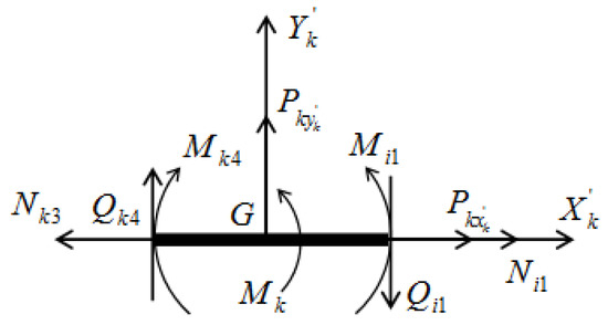
Figure 7.
Rigid joint with constant cross-sections of the element, where the external concentrated loads are attached.
5. Decisive Equations for Determining Internal Forces
By combining the equations of the equilibrium of the elements and joints into one system, we obtain the equilibrium equations for the entire discrete model of the mechanism. They can be written in the general form:
These systems of equations are sufficient for determining internal forces in links of mechanisms with statically determinate structures. The matrix of equilibrium equations for the discrete model of the mechanisms consists of the matrices of the equilibrium equations of their individual elements, as well as the equilibrium equation of their joints. The matrix of the equilibrium equations for the discrete models of mechanisms is as follows:
The vector of load and the vector of the force in the calculated cross-sections of the discrete models of the mechanisms are formed from the vectors of the load and the forces in the calculated cross-sections of their individual elements. These vectors in the vector form have the following form:
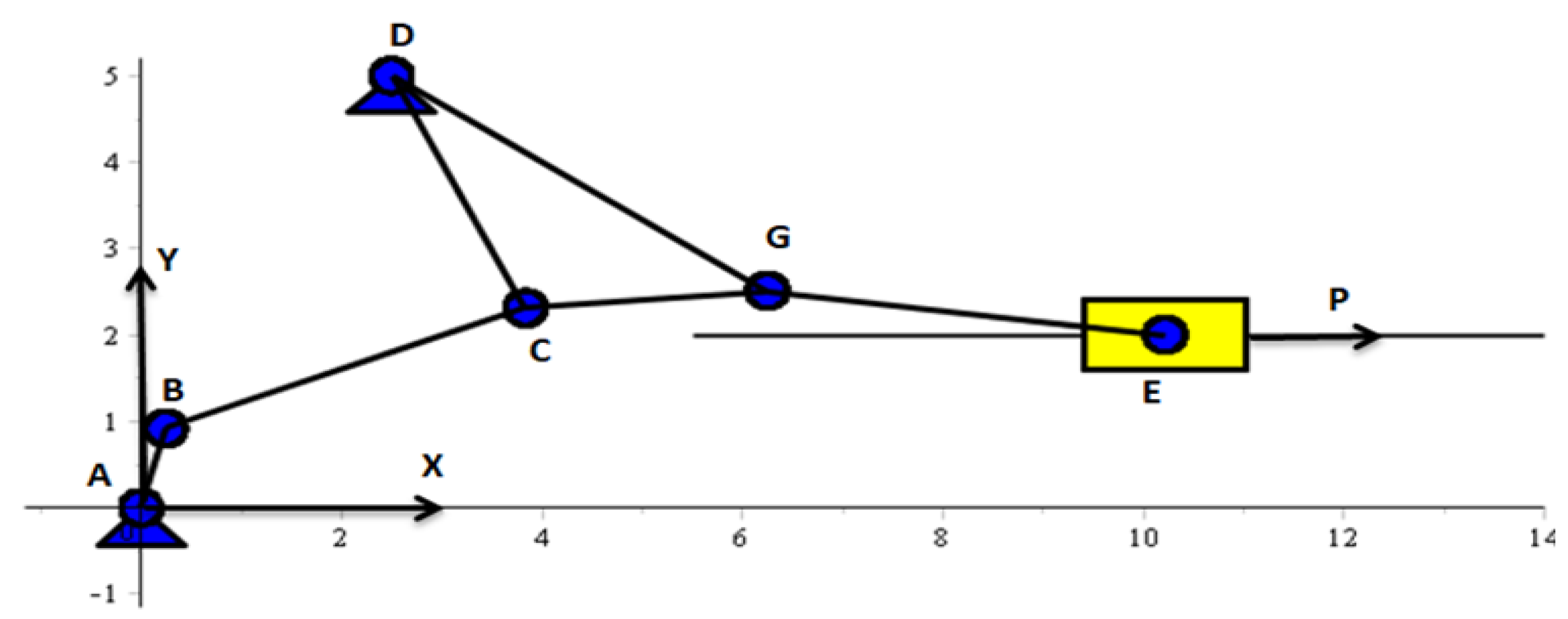
Determination of internal forces will be outlined using an example of a second-class six-bar linkage with one driving link, shown in Figure 8. Computer programs were developed in the Maple system to determine and construct the diagrams of inertial and internal forces on the links. The resulting inertial and internal forces are shown in Figure 8, Figure 9, Figure 10, Figure 11, Figure 12 and Figure 13 for some positions of the mechanism.
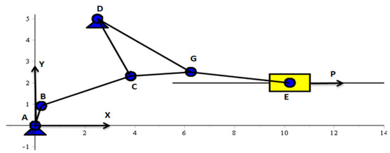
Figure 8.
The second-class six-bar mechanism with one driving link.
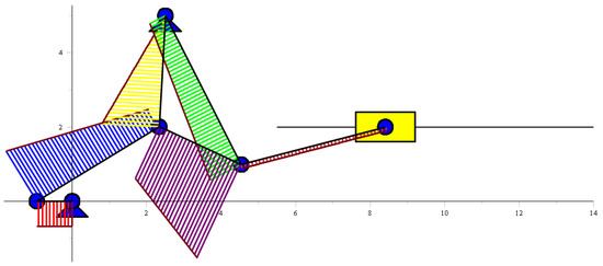
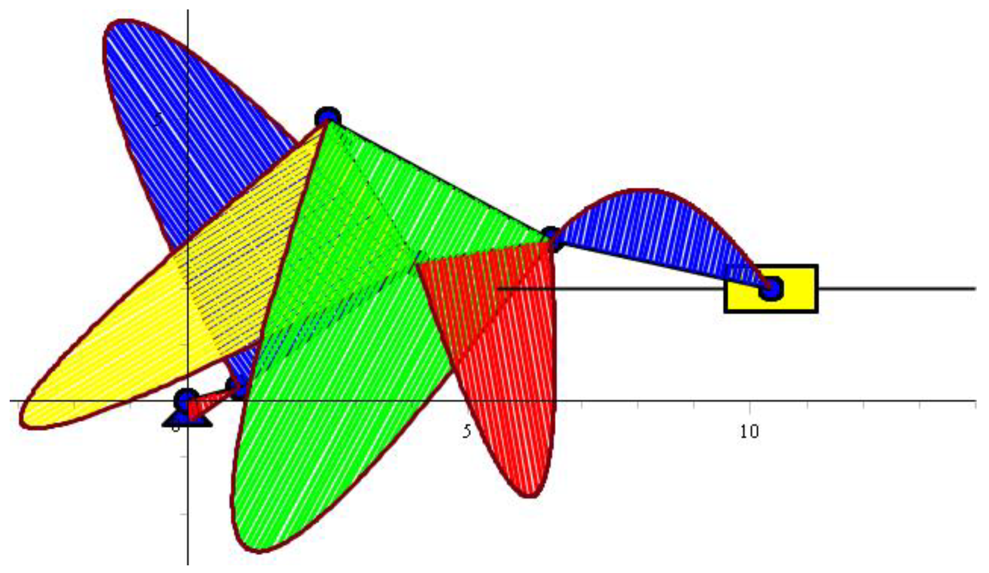
Figure 9.
The mechanism under discussion of the links showing the constructed transverse dynamic distributed loads.
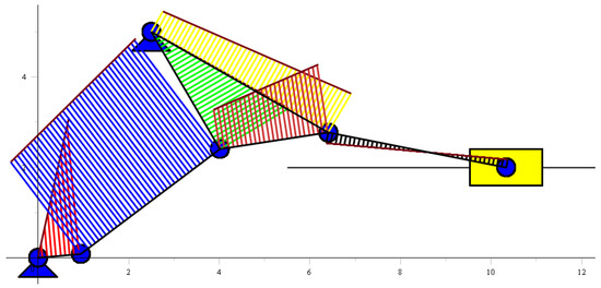
Figure 10.
The mechanism of the links illustrating the constructed longitudinal dynamic distributed loads.

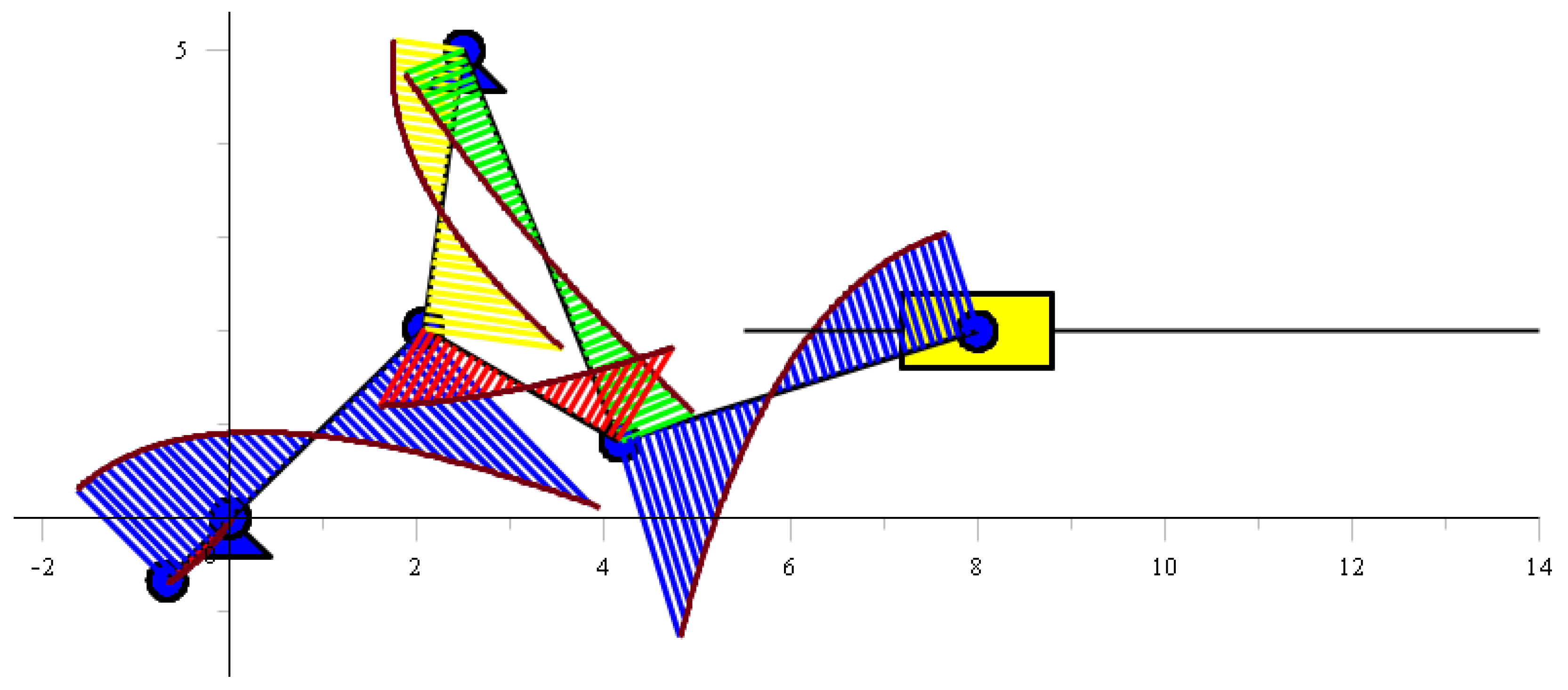
Figure 11.
The mechanism of the links showing the constructed bending moments.
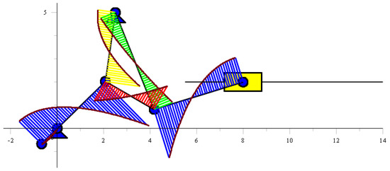
Figure 12.
The mechanism of the links showing the constructed shearing force.
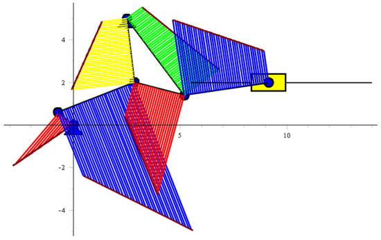
Figure 13.
The mechanism of the links showing the constructed normal force.
6. Results and Discussion
To verify our developed theory, we applied the theory to solving a task involving a specific six-bar linkage. We solved the kinematics problem and determined the internal forces in the links, as well as animated the motion and constructed the diagrams of the distributed dynamic loads and internal forces on the links. Thus, we wanted to show that our developed theory works and determine the dynamic loads and the internal forces in the links, depending on how the mechanism position changes. To determine the maximum values of the internal forces, it was necessary to determine internal forces in all positions of the mechanism and manipulator. The maximum values of internal forces allow, according to the appropriate strength theories, to select the shape and find linear dimensions of the cross-sections of the links. The validity of the results can be seen from the plotted diagrams, for example, in Figure 11 in the cross-section A of the link 1. The driving moment is shown and the moment in the cross-section B is zero, since there is a rotational kinematic pair. Since there are differential dependencies between the distributed transverse dynamic loads, the shearing force, and the bending moment, using these relationships all the diagrams can be checked. For example, in Figure 12, in the cross-section of link 2 where the shearing force is zero, the bending moment in the same cross-section in Figure 11 has a maximum value and so on.
7. Conclusions
In this study, we established the laws of distribution of the distributed loads from inertial forces and forces of gravity, arising from the distributed weight of the links with constant cross-sections. Dependencies between the distributed loads and with geometrical, physical, and kinematic characteristics of the links were determined. The approximation matrix of the internal forces of the element under the action of distributed loads with trapezoidal shape intensity was found. The approximation matrices of the internal forces define the relationship between the vector of the force in any cross-section of the element and the vector of forces in the calculated cross-sections . The computational and discrete schemes of the linkage mechanisms for elastic calculation were developed. The dynamic equations of equilibrium for the discrete model of each element, as well as the dynamic equations of equilibrium for hinged and rigid joints, under the action of transverse and longitudinal distributed trapezoidal loads, were derived. In the dynamic equilibrium equations of the discrete model of the elements, the connections were established between the components of the vector of the forces in the calculated cross-sections and with geometric, physical, and kinematic characteristics of links with constant cross-sections, in their plane-parallel movement. Decisive equations were derived for determining internal forces in the links of the mechanisms with a statically determinate structure. In using the developed technique, programs were created in the Maple system and animations of the motion of the mechanisms were produced. The links were constructed with the intensity of the distributed transverse and longitudinal dynamic loads, the bending moments, and the shearing and normal forces, depending on the kinematic characteristics of the links.
Author Contributions
M.U. established the laws of distribution of distributed dynamic loads, received the approximation matrix of internal forces of the element; developed the computational discrete model of elastic calculation of mechanisms and manipulators; M.U. and T.S. derived the dynamic equilibrium equations of the discrete model of the element; Z.B., S.Z. and S.P. derived the dynamic equilibrium equations for hinged and rigid joints; M.U., T.S. and Z.B. received the decisive equations for determining internal forces in the links of mechanisms and manipulators; M.U., S.Z. and S.P. created the programs in the MAPLE and solved the problem for the specific six-bar linkage with the solution of the kinematics problem and with the determination of internal forces in the links, as well as with the animation of motion and with the construction of the diagrams of distributed dynamic loads and internal forces on the links. All authors contributed equally to the evaluation of the results and writing of this paper.
Funding
This research received no external funding.
Conflicts of Interest
The authors declare no conflicts of interest.
References
- Tschiras, A.A. Structural Mechanics; Stroyizdat: Moscow, Russia, 1989; ISBN 5-274-00555-1. [Google Scholar]
- Darkov, A.V.; Shaposhnikov, N.N. Structural Mechanics; Lan’: St. Petersburg, Russia, 2010; ISBN 978-5-8114-0576-3. [Google Scholar]
- Shakirzyanov, R.A.; Shakirzyanov, F.R. Lecture Notes in Structural Mechanics; KGASU: Kazan, Russia, 2014. [Google Scholar]
- Neubert, V.H.; Hahn, H.T.; Lee, H. Lumped parameter beams based on impedance methods. J. Eng. Mech. Div. 1970, 96, 69–82. [Google Scholar] [CrossRef]
- Golebiewski, E.P.; Sadler, J.P. Analytical and experimental investigation of elastic slidercrank mechanisms. J. Eng. Ind. 1976, 98, 1266–1271. [Google Scholar] [CrossRef]
- Sadler, J.P. A Lumped Parameter Approach in the Kineto-Elastodynamic Analysis of Mechanisms. Ph.D. Thesis, Rensselaer Polytechnic Institute, New York, NY, USA, 1972. [Google Scholar]
- Sadler, J.P.; Sandor, G.N. A lumped parameter approach to vibration and stress analysis of elastic linkages. J. Eng. Ind. 1973, 95, 549–557. [Google Scholar] [CrossRef]
- Sadler, J.P.; Sandor, G.N. Nonlinear vibration analysis of elastic four-bar linkages. J. Eng. Ind. 1974, 96, 411–419. [Google Scholar] [CrossRef]
- Zienkiewicz, O.; Taylor, R.; Zhu, J. The Finite Element Method: Its Basis and Fundamentals; Butterworth-Heinemann: Oxford, UK, 2013; ISBN 978-0-0809-5135-5. [Google Scholar]
- Strang, G.; Fix, G. An Analysis of the Finite Element Method; Wellesley-Cambridge Press: Wellesley, MA, USA, 2008; ISBN 978-0-9802-3270-7. [Google Scholar]
- Tokhi, M.O.; Mohamed, Z.; Amin, S.H.M.; Mamat, R. Dynamic Characterizaion of a Flexible Manipulator System: Theory and Experiments. Available online: https://zapdf.com/dynamic-characterisation-of-a-flexible-manipulator-system-th.html (accessed on 4 September 2018).
- Tokhi, M.O.; Mohamed, Z.; Shaheed, M.H. Dynamic characterization of a flexible manipulator system. Robotica 2001, 19, 571–580. [Google Scholar] [CrossRef]
- Chung, J.; Yoo, H.H. Dynamic analysis of a rotating cantilever beam by using the finite element method. J. Sound Vib. 2002, 249, 147–164. [Google Scholar] [CrossRef]
- Shaker, M.C.; Ghosal, A. Nonlinear modeling of flexible manipulators using non-dimensional variables. J. Comput. Nonlinear Dyn. 2006, 1, 123–134. [Google Scholar] [CrossRef]
- Yue, S.; Tso, S.K.; Xu, W.L. Maximum dynamic payload trajectory for flexible robot manipulators with kinematic redundancy. Mech. Mach. Theory 2001, 36, 785–800. [Google Scholar] [CrossRef]
- Korayem, M.H.; Haghpanahi, M.; Heidari, H.R. Maximum allowable dynamic load of flexible manipulators undergoing large deformation. Sci. Iran. 2010, 17. Available online: http://scientiairanica.sharif.edu/article_3246.html (accessed on 04 September 2018).
- Korayem, M.H.; Haghpanahi, M.; Heidari, H.R. Maximum allowable load of very flexible manipulators by using absolute nodal coordinate. Aerosp. Sci. Tech. 2015, 45, 67–77. [Google Scholar] [CrossRef]
- Du, Z.; Yu, Y.; Yang, J. Analysis of the Dynamic Stress of Planar Flexible-Links Parallel Robots. Front. Mech. Eng. China 2007, 2, 152–158. [Google Scholar] [CrossRef]
- Dwivedy, S.K.; Eberhard, P. Dynamic analysis of flexible manipulators: A literature review. Mech. Mach. Theory 2006, 41, 749–777. [Google Scholar] [CrossRef]
- Li, H.; Hao, G. Constraint-Force-Based Approach of Modelling Compliant Mechanisms: Principle and Application. Precis. Eng. 2016, 47, 158–181. [Google Scholar] [CrossRef]
- Utenov, M.U. Investigations of forces, arising from the self mass of links with constant and variable cross-sections in their plane-parallel motion. In Proceedings of the First International Scientific and Practical Conference, Almaty, Kazakhstan, 18–19 October 2000. [Google Scholar]
- Utenov, M.U. The matrix of approximation of element force under the action of distributed load with parabolic intensity. In Proceedings of the First International Scientific and Practical Conference, Almaty, Kazakhstan, 18–19 October 2000. [Google Scholar]
- Utenov, M.U. Construction of discrete models of planar rod mechanisms in the elastic calculation. Bull. Kazakh Acad. Transp. Commun. 2001, 6, 61–64. [Google Scholar]


© 2018 by the authors. Licensee MDPI, Basel, Switzerland. This article is an open access article distributed under the terms and conditions of the Creative Commons Attribution (CC BY) license (http://creativecommons.org/licenses/by/4.0/).