Workspace Limiting Strategy for 6 DOF Force Controlled PKMs Manipulating High Inertia Objects

Abstract

This article describes an efficient and effective strategy for limiting the workspace of a six degrees of freedom parallel manipulator, with challenging motion smoothness requirements due to both the high inertia objects carried by the end effector and the pose references coming from a force feedback loop. Firstly, a suitable formulation of the workspace is studied, distinguishing between different conventions and procedures. Thereafter a discrete and analytical formulation of the workspace is obtained and developed in order to suit this application. Having obtained the limits, a methodology to evaluate the robot pose is discussed, taking into account the reference pose buffering technique and the real time pose estimation through the numeric solution of the nonlinear forward kinematics equations. The safety algorithm designed checks the actual robot pose and future poses to be commanded, and takes control of the reference pose generation process, if an exit of the safety workspace is detected. The result obtained is a soft compliant surface within which the robot is free to move, but outside of which a “force field” pushes the robot end-effector to return smoothly. To reach this objective, the control deflects the end effector trajectory safely and smoothly and moves it back to within the workspace limits. Nevertheless, this preserves the continuity of the velocity and controls the acceleration, to avoid dangerous vibrations and shocks. Simulation and experimental result tests are conducted to verify the algorithm effectiveness and the efficient implementation.

1. Introduction

This work is one of the results obtained from the development of a new Hardware-in-The-Loop (HIL) system for the European H2020 project named LIFES50+ [1]. The aim of this project is to prove cost effective technology for floating substructures for 10 MW [2] offshore wind turbines, at water depths greater than 50 m. In particular, the objectives are optimizing and qualifying two innovative substructure designs for 10 MW wind turbines. Within this project, the Politecnico di Milano has designed a novel real time HIL experimental setup, whose aim is to test the scaled model of a 10 MW wind turbine inside a wind tunnel test facility, emulating the dynamic behaviour of the floating substructure by means of a robotic device.

HIL is a fundamental tool for both hardware and software component developments [3], combining many advantages of both physical and virtual prototyping, allowing rapid, accurate and economic development of increasingly complex and integrated systems. The basic idea of this technique is to test a single real component or subsystem, cooperating with virtual or emulated part of the complete system or environment. Examples of HIL devices can be found in many different fields, ranging from flight simulation, through to military/space applications [4] and automotive ones. In the latter field examples include single subsystems to test active/passive suspensions, engines [5], power trains, tires, brakes with Anti-lock-Braking-System (ABS) or Electronic-Stability-Program (ESP) control systems, Driver-In-the-Loop virtual simulations [6], immersing real cockpit or even complete vehicles in virtual environments.

The HIL proposed setup allows one to reproduce within the wind tunnel, the dynamic effects of both aerodynamic and hydrodynamic loads, acting respectively on the real (scaled wind turbine) and simulated (floating substructure and sea environment) parts of the system. The output motion of the floater dynamic model is imposed to the turbine thanks to a six Degree-Of-Freedom (DOF) parallel manipulator, named Hexafloat [7], controlled in closed real time loop with the dynamic model of the floater and the real loads generated by the wind [8].

The primary task of the robot is to carry the wind turbine model, emulating the behaviour of the floating substructure immersed in the sea environment. During this task, the control software has to guarantee a high level of safety and performance [9]. In particular, special attention is required for the motion generation in terms of fluidity (velocity continuity) and acceleration limits. In fact, unexpected discontinuities in velocity or excessive accelerations imposed to the robot could cause dangerous vibrations, invalidating the test measurements and generating potentially hazardous situations. Multiple sources can lead to this problem: trajectory planning and motion blending failure in the presence of unpredictable reference generation and force input, communication issues, procedural mistakes, numerical problems and saturation. All these can potentially cause great accelerations to be commanded at the base of the wind turbine. Multiple safety algorithms and specific software tools have been developed to ensure optimum performance and safety requirements of this challenging HIL application. The one treated in this article belongs to the safety routines and deals with the task of limiting robot movements inside a specific workspace.

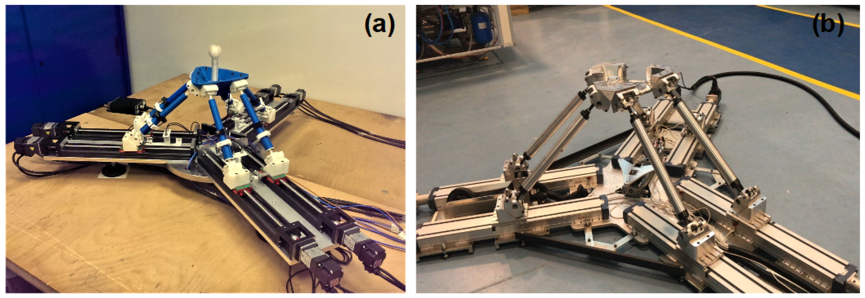
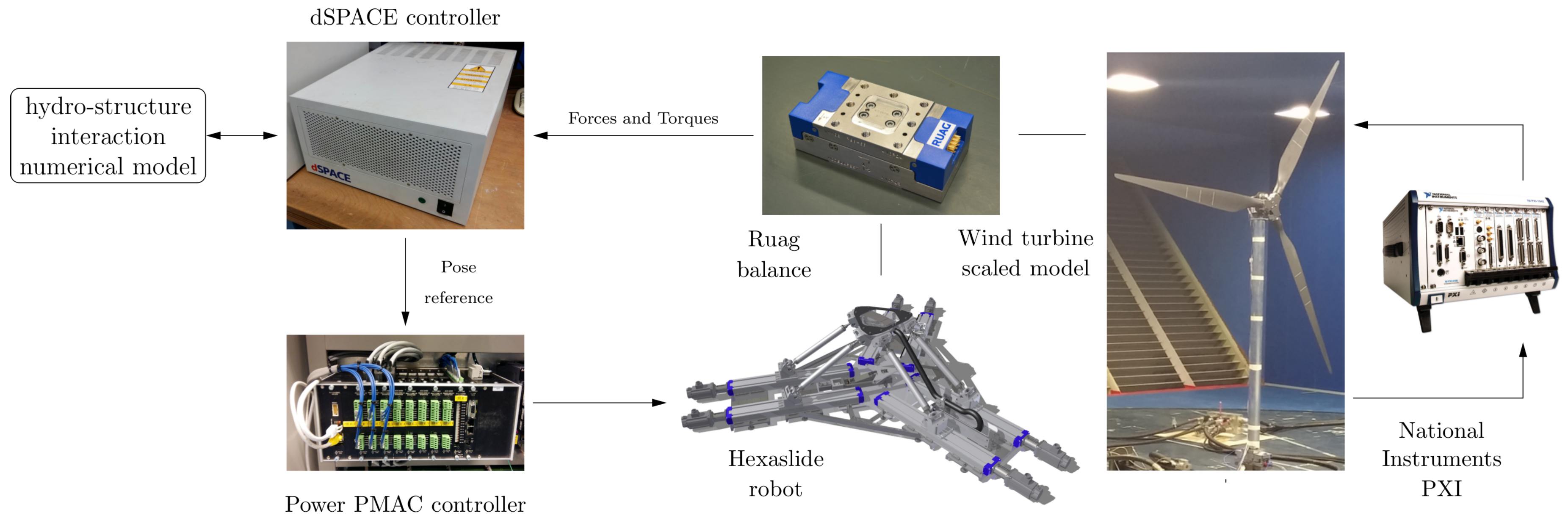
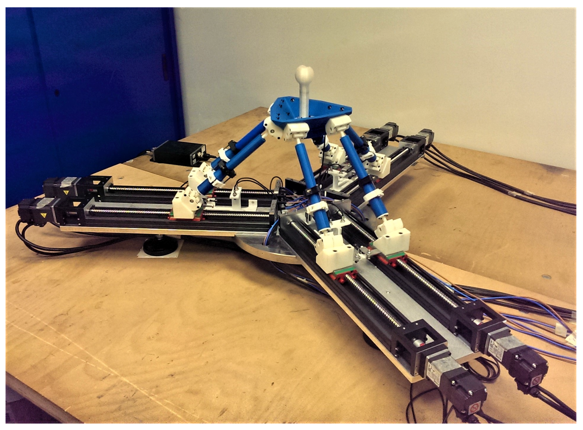
2. Hexafloat Robot Description

Two robots have been designed and realized for the purposes of this project, both shown in Figure 1. The first one is installed below the wind tunnel floor and properly dimensioned for HIL tests in the contest of the LIFES50+ experimental activities [10,11,12]. The second robot is a 1:3 faithful scaled reproduction of the first installed in a laboratory and designed to develop, verify and optimize the control and safety algorithms without the use of the wind tunnel. Multiple requirements have been taken into account during the robot design and optimization. Extensive description of the optimization process is provided in [11,13,14,15].

The result of the design process is a fully parallel six DOF robot, based on the PUS (PRRS) joints configuration, actuated by six direct drive brushless motors, that realize six prismatic joints by means of direct ballscrew–slider connection. All the actuators are ground connected to reduce overall inertia and improve dynamic capabilities. A six axis force/torque sensor will be the interface between the turbine and robot’s end-effector. The robot, due to its architecture, is fully developed under the turbine model, reducing its influence on air flow quality, even considering that it will be mounted below the wind tunnel floor level. The high level control software and tools together with position and velocity servo loops, have been implemented on a Power PMAC motion controller, property of Omron Delta Tau, while the torque/current loop and phase commutation are controlled by six servo controller. Floater dynamic model real time integration is performed by a dedicated dSPACE controller, while turbine management is handled by a completely independent PXI controller by NI. Refer to Figure 2 for a simplified scheme of the HIL setup.

Since kinematics and kinetostatics equations will be used inside workspace formulation, a brief summary of the main constraint equations is provided. Refer to Figure 3 for a simplified scheme of the Tool-Centre-Point (TCP) geometric parameters; refer instead to Figure 4 for vectorial closures of each kinematic chain and reference frames, and to Equation (2) for the analytical solution of the i-th inverse kinematics problem. In

Table 1. Components of the unitary orientation vectors of the guides, expressed in the global reference frame.

${\widehat{\mathit{u}}}_1$	${\widehat{\mathit{u}}}_2$	${\widehat{\mathit{u}}}_3$	${\widehat{\mathit{u}}}_4$	${\widehat{\mathit{u}}}_5$	${\widehat{\mathit{u}}}_6$
1	1	$-1/2$	$-1/2$	$-1/2$	$-1/2$
0	0	$\sqrt{3}/2$	$\sqrt{3}/2$	$-\sqrt{3}/2$	$-\sqrt{3}/2$
0	0	0	0	0	0

the unitary vectors components representing actuation direction in the global reference frame are provided. In

Table 2. Optimized geometrical parameters of the actual and scaled robot.

Parameter	Value
	Actual	Scaled
Home position height $z_{WSd}$	463 mm	154.3 mm
Half-distance between base joints centers s	203 mm	67.7 mm
Links length l	686.6 mm	228.9 mm
Platform joints radius $R_p$	238.71 mm	79.6 mm
Platform joints angle ${\theta }_p$	38.474°	38.5°

are reported the major geometrical parameters for both full scale and scaled machine.

$${\mathbf{d}}_i=\mathbf{p}+\left[R\right]{\mathbf{b}}_i^{\prime }-{\mathbf{s}}_i$$

(1)

$$q_i={\mathbf{d}}_i^T{\widehat{\mathbf{u}}}_i+\sqrt{{\mathbf{d}}_i^T({\widehat{\mathbf{u}}}_i{\widehat{\mathbf{u}}}_i^T-\left[I\right]){\mathbf{d}}_i+l_i^2}$$

(2)

In Equation (1), the $\mathbf{p}$ and $\left[R\right]$ terms represent, respectively, the position vector and the orientation matrix of the end-effector.

The study of the dynamic model of the floating substructure has highlighted the need of a parallelepiped-shaped nominal workspace, obtained imposing three upper limits and three lower limits to the three translational degrees of freedom. These limits represent the volume in which the robot must be able to assume all the possible orientations obtained combining the three angle ranges expressed in

Table 3. Technical specifications for the nominal workspace.

Workspace	Specifications
Surge x	$\pm 150$ mm
Sway y	$\pm 75$ mm
Heave z	$\pm 75$ mm
Roll $\alpha$	$\pm 5$
Pitch $\beta$	$\pm 8$
Yaw $\gamma$	$\pm 3$

and preserving an optimum kinematic behaviour. The limits expressed in Table 3 refer to the full scale machine: for the scaled one, about which the results will be provided, the translations ranges have to be downscaled by a $1/3$ factor, while rotations ranges remain the same. These requirements have been used during the geometric optimization of the machines, and constitute also the starting point for the formulation of the safety limit for the workspace.

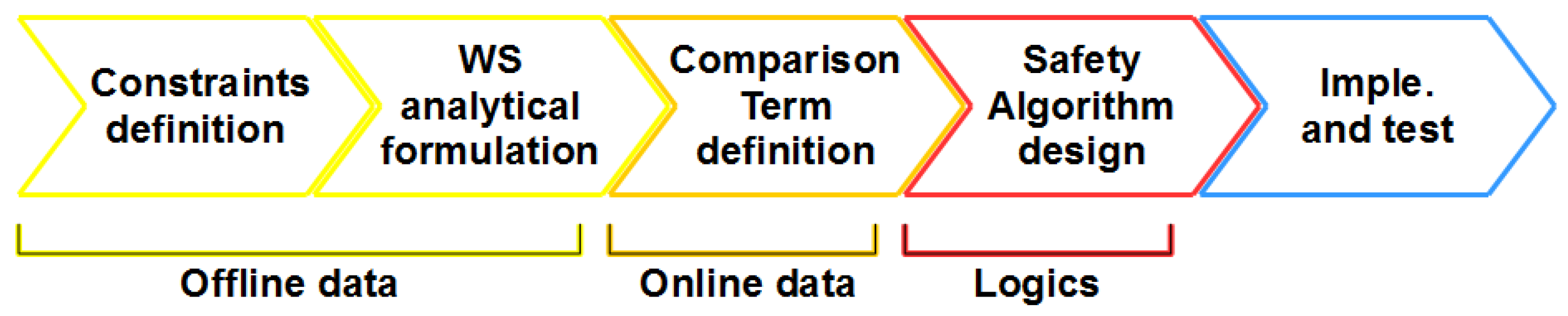
3. Workspace Safe Limiting

The first fundamental step for this algorithm is to find an analytical and convenient formulation of the acceptable WorkSpace (WS) for the six DOF robot Hexafloat. Depending on the boundaries conditions chosen and on the formulation method, multiple WS are definable. Moreover, once the analytical definition of the WS has been found, it is necessary to define how to use this limit in order to respect the safety requirements of the application and how to monitor the end-effector position with respect to it. Finally, the designed safety algorithm has to be implemented and tested in order to verify efficiency and performance. All of these steps are graphically summarized in Figure 5 .

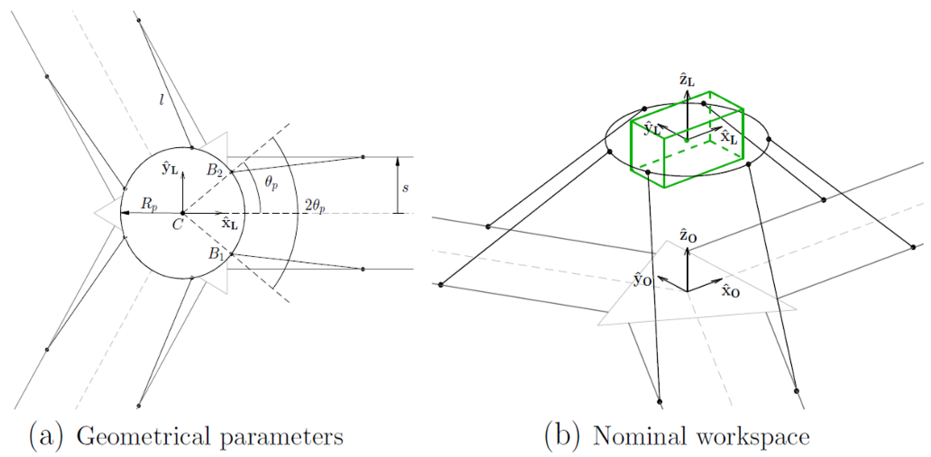
3.1. Workspace Analytical Formulation

The complete workspace of a PKM with six DOF is a six-dimensional space which can not be directly related to a 3-D representation. For this reason, different types of subsets of the complete workspace are usually determined. The most commonly determined workspace is the constant- orientation workspace, which is the three-dimensional volume that can be attained by the TCP when the mobile platform is maintained at a constant orientation [16]. If the platform orientation is null, the zero-orientation workspace is obtained. For this particular application, we study and determine the total-orientation workspace that corresponds to the volume within which all possible orientations determined by the combinations of the three orientation angles varying in a given range are guaranteed [17]. Many methods are available in the literature to determine the total-orientation workspace and they are based essentially on two different approaches:

• geometrical approach, as made by Gosselin for the Gough–Stewart hexapod computing the so-called vertex space [18] and applied by Bonev [16], or as introduced in [19]; and
• numerical approach based on discretization [20,21].

The former is potentially fast and accurate, while the accuracy of the latter depends on how fine the discretization is. Even though numerical approach is computationally demanding, for our application, the calculation associated will be performed only once and off-line, so it has been preferred over the geometrical approach due to implementation simplicity. The numerical method requires a proper space discretization in order to verify constraints equations at a finite number of points. In order to express the coordinates of each point, it is convenient to adopt a spherical coordinate system positioned in the centre of the nominal workspace, whose parameters are the radius r, the azimuth $-{90}^{\circ }\le \phi \le {90}^{\circ }$, and the elevation $0^{\circ }\le \theta \le {360}^{\circ }$. In Figure 6, the relationship between local spherical coordinate system and Cartesian reference frames is shown, togheter with azimuth and elevation angles. Every time a point is investigated, it will be included inside total-orientation-workspace only if a set of constraints are satisfied:

• Kinematic constraints:

  -

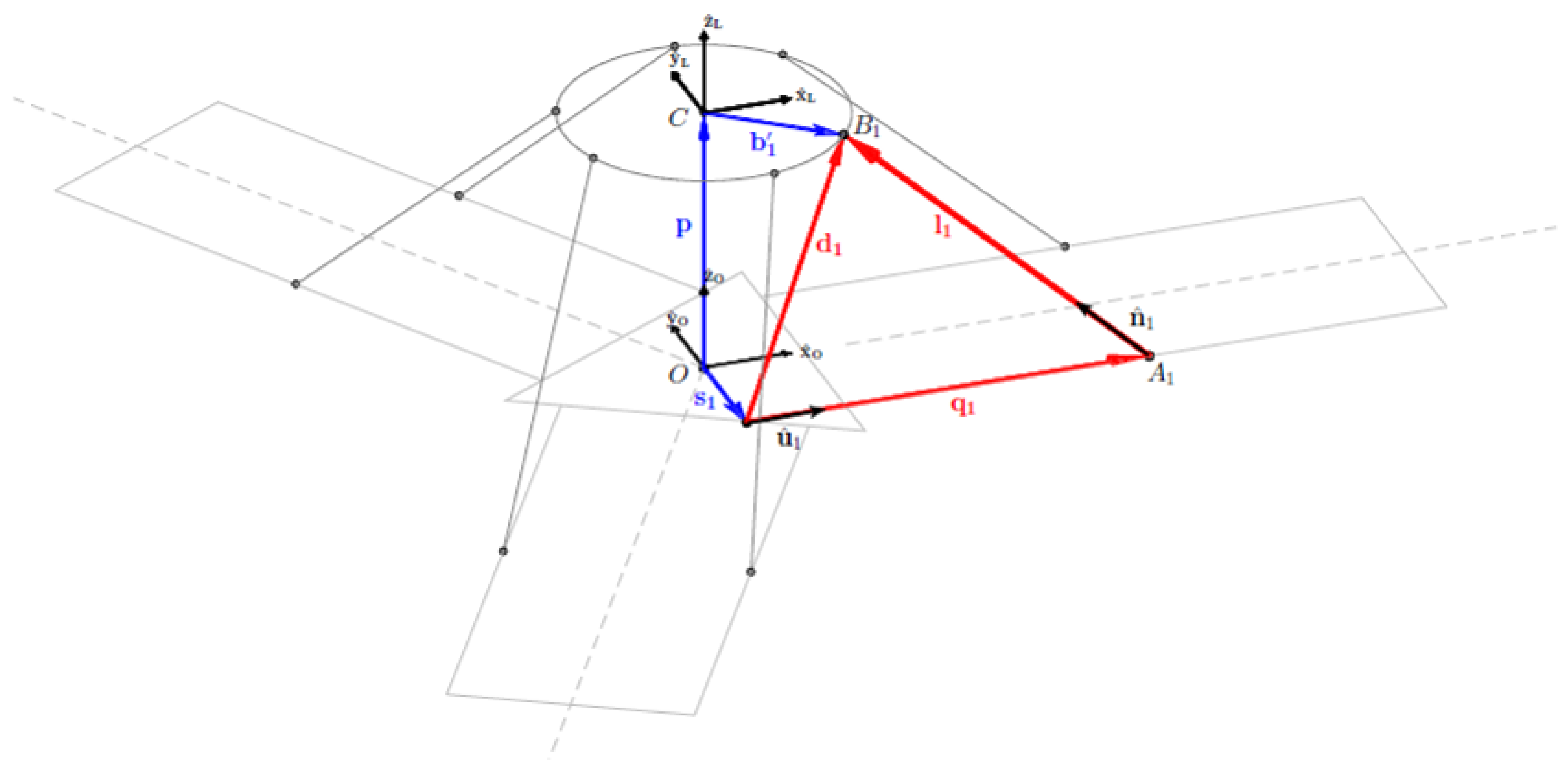
  ${\Delta }_i\ge 0$: with reference to Equation (2), ${\Delta }_i={\mathbf{d}}_i^T({\widehat{\mathbf{u}}}_i{\widehat{\mathbf{u}}}_i^T-\left[I\right]){\mathbf{d}}_i+l_i^2$. This condition is relative to top-base joints distance consistency with respect to links length.

  -

  Actuated joints range of motion.

  -

  Passive universal joints range of motion.

• Kinetostatic constraints:

  -

  Maximum multiplication of external loads. This criterion is based on limiting ${\left|\right|\left[J\right]}^{-T}{\left|\right|}_{\infty }$ starting from ${\mathbf{f}}_{\mathbf{c}}=\left[J\right]{\mathbf{Ø}}_{\mathbf{a}}$ that bounds the external loads to the actuation torques ${\mathbf{Ø}}_{\mathbf{a}}$ through the Jacobian matrix $\left[J\right]$, obtained by differential kinematics analysis.

The algorithm that computes the total-orientation workspace requires verifying that, for each point, the robot can guarantee all the possible orientations in the range in which it has been designed for. The algorithm procedure is summarized in the following steps:

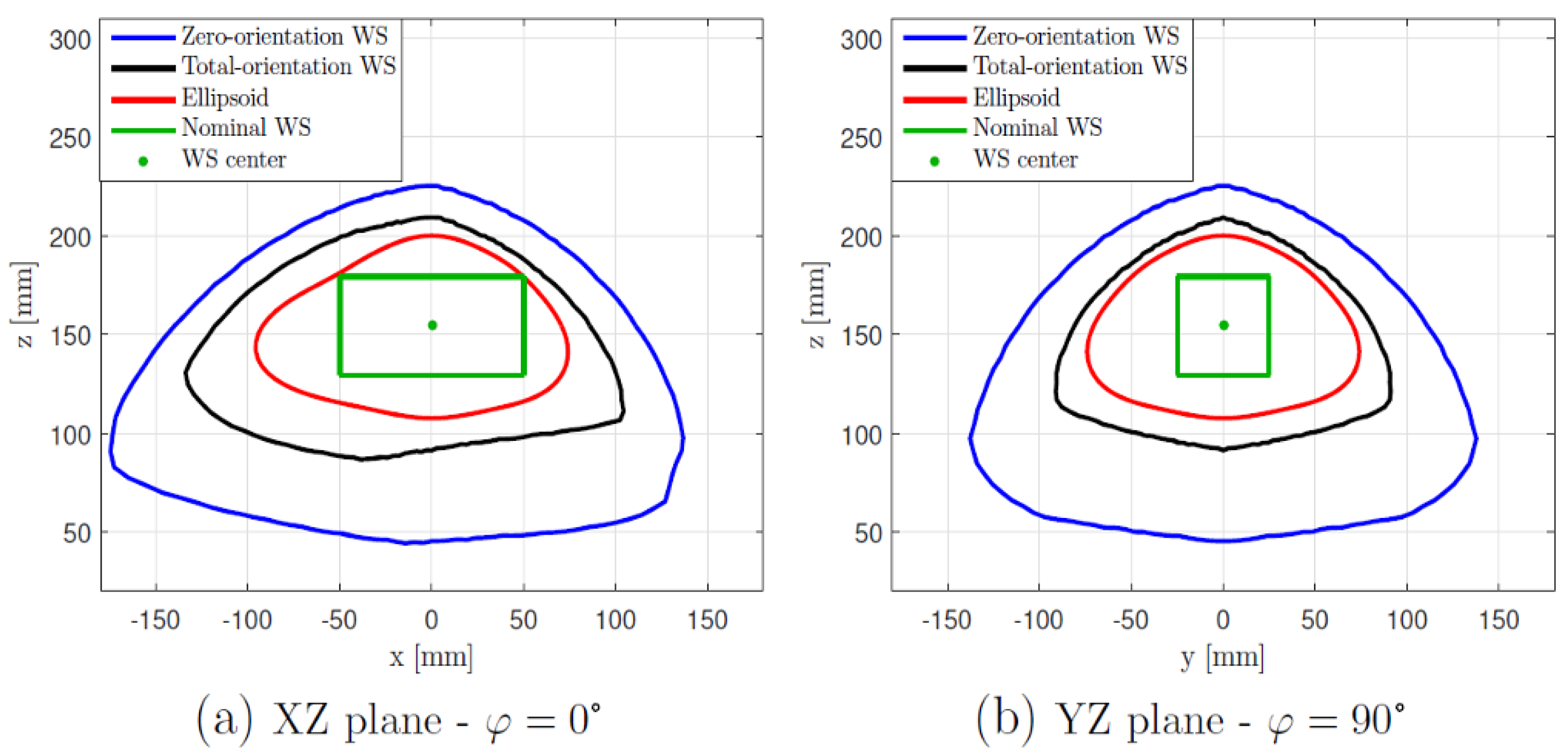
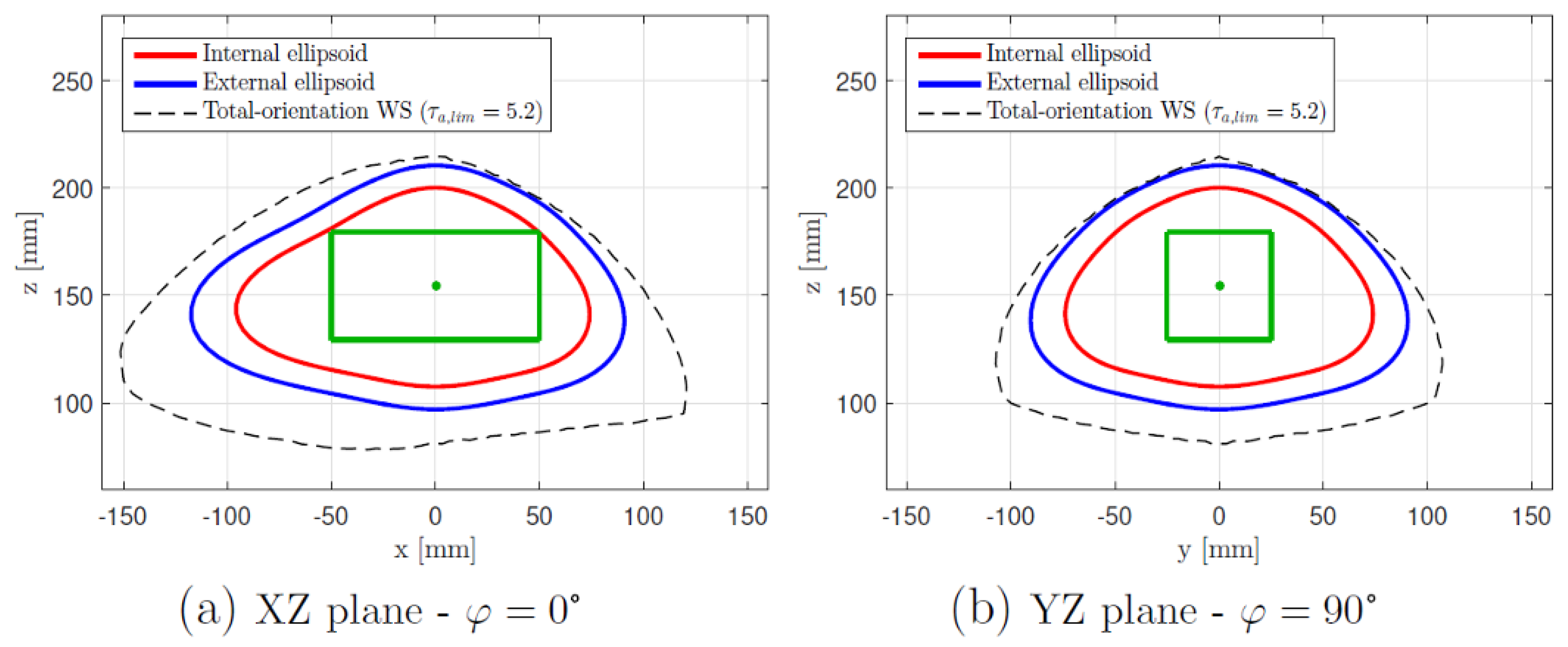
• both the ranges of $\phi$ and $\theta$ are properly discretized through the chosen resolution $\Delta \phi$ and $\Delta \theta$;
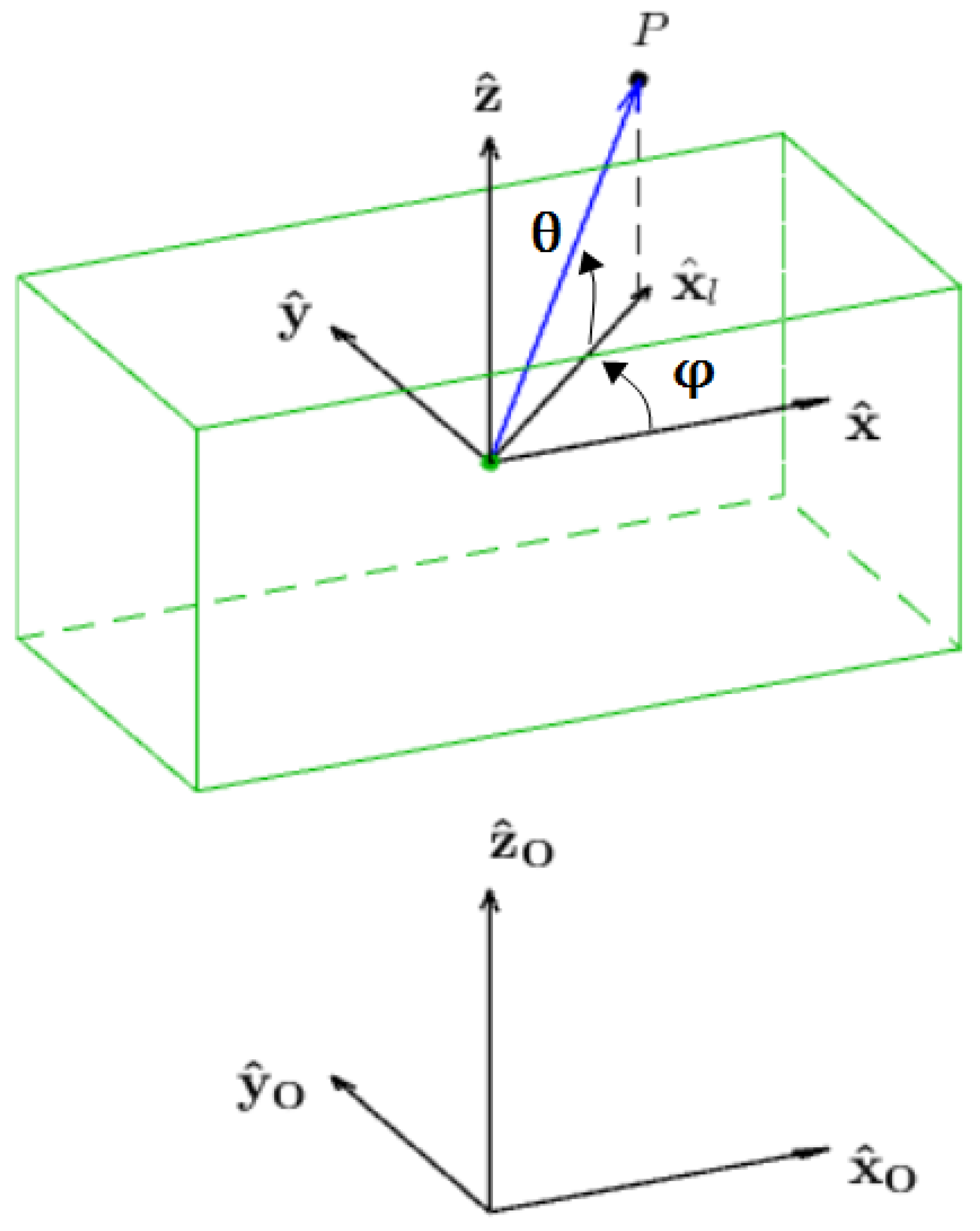
• a proper value of $r_{max}$ is chosen as the radius of a spherical surface that contains the whole total-orientation workspace;
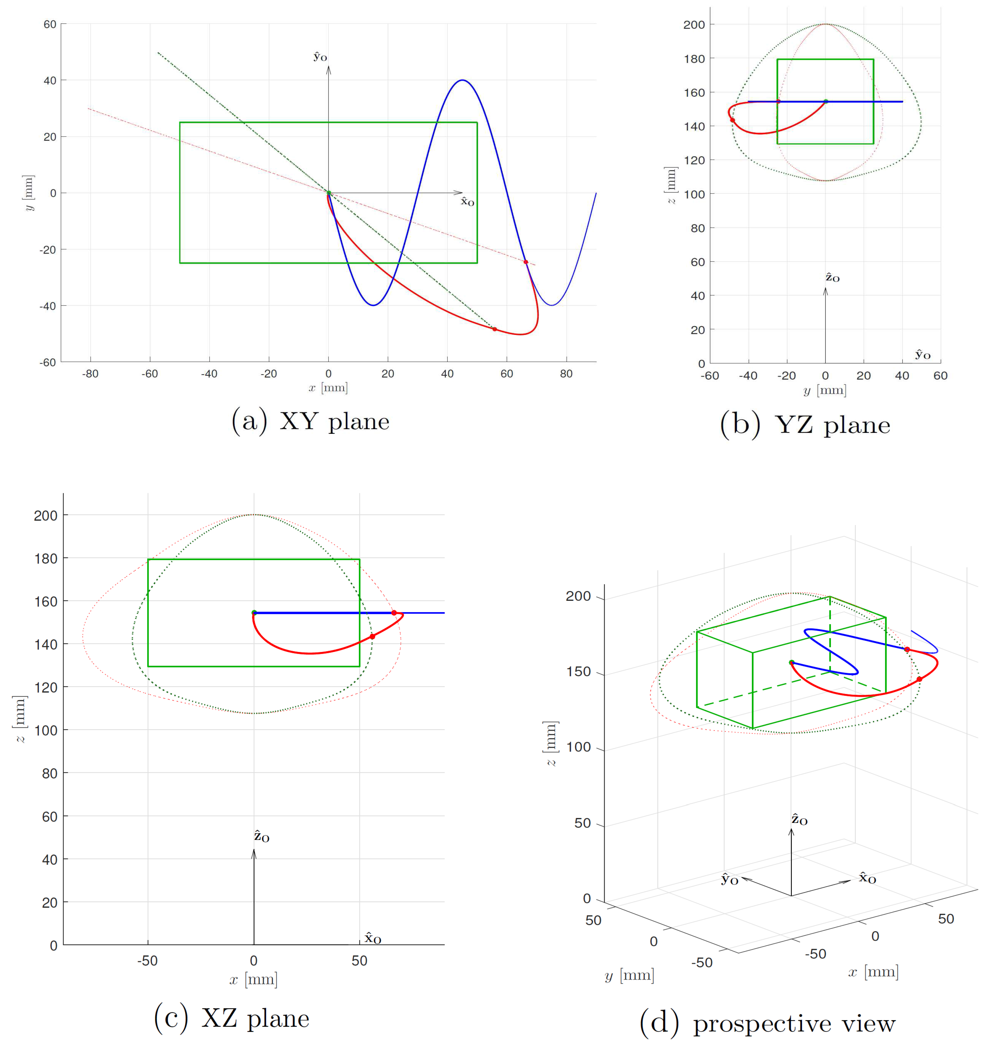
• for each plane identified by ${\phi }_i$, all the values ${\theta }_j$ are analysed. For each combination, the point P determined by the parameters $\{r,{\phi }_i,{\theta }_j\}$ is considered, as shown in Figure 6.
• for each point, all the possible combinations of orientation inside the given range must be evaluated, which means that the orientation angles also have to be discretized with a proper resolution;
• if all the constraints are satisfied for each possible orientation, the point is contained in the total-orientation workspace: the value of r is saved in a proper matrix and the algorithm proceeds with the next value of ${\theta }_j$ or with the next value of ${\phi }_i$ if all the values ${\theta }_j$ have been analysed for the current plane;
• if at least one constraint is violated, the algorithm stops the calculations for the current set of parameters $\{r,{\phi }_i,{\theta }_j\}$, and the point P is rejected and the value of the radius r is decreased of a proper step $\Delta r$; and
• the algorithm stops when all the values ${\phi }_i$ have been evaluated.

For every plane identified by a value of $\phi$, the result of the process is a section of the total-orientation WS made by the set of maximum admissible radius associated to each value of $\theta$. This radius map is not related to an analytical formulation at this stage, therefore is necessary to obtain the equation of a 3-D surface more easily usable in a safety algorithm. For this reason a 3-D ellipsoid has been modified in order to fit the shape of the discretized volume computed and obtain a more conservative analytical limit. Figure 7 shows a comparison between analytical result, nominal WS and the zero and total discretized WS. The analytical limit exploits well the space available with a continuous surface.

The resulting modified ellipsoid is defined by the nonlinear equation:

$$r_e=f(\mathbf{a},\phi ,\theta )$$

(3)

where $\mathbf{a}$ is a vector of constant coefficients. The components of the vector $r_e$ on the local frame axis are:

$$\begin{array}{cc}\hfill r_{e,x}& =r_{e}cos\theta cos\phi \hfill \\ \hfill r_{e,y}& =r_{e}cos\theta sin\phi \hfill \\ \hfill r_{e,z}& =r_{e}sin\theta \hfill \end{array}$$

(4)

3.2. Robot Pose Monitoring

The next step for building a safety algorithm is to determine what is to be compared with the analytical 3-D limit computed. The real-time monitoring of the limits require knowledge of the actual position and orientation of the TCP. Since direct measure of the pose is a challenging task, the combination of numerical estimation and buffering technique has been implemented. First, the nonlinear forward kinematics equation has been solved: to estimate TCP pose in real-time, a fast and stable numeric algorithm has been implemented in C language, based on Jacobian-Free-Monotonic-Descent-factor (JFMD) [22]. This algorithm assures convergence even for initial guesses far from the actual solution and time approximately with a computation time of 50 $\mathsf{\mu }$s, suitable for real-time pose estimation at the servo frequency of 1.6 kHz.

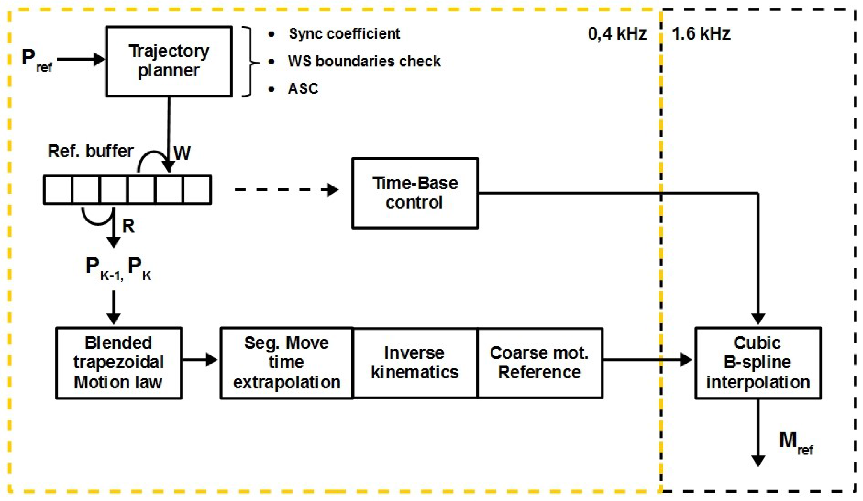
3.3. Motion Planner

The actual safety routine is implemented inside an high performance Motion-Planner architecture, described in Figure 8. This architecture features three main control levels [23]. The highest level is occupied by the Trajectory-Planner, or the group of safety algorithms that analyse and eventually modify the pose references coming from dynamic model integration. Besides WS boundaries check, highlighted in red in Figure 8, two more algorithms act at this level, featuring a synchronization coefficient between first reference coming from outside and robot starting pose, and Acceleration-Saturation-Control (ASC).

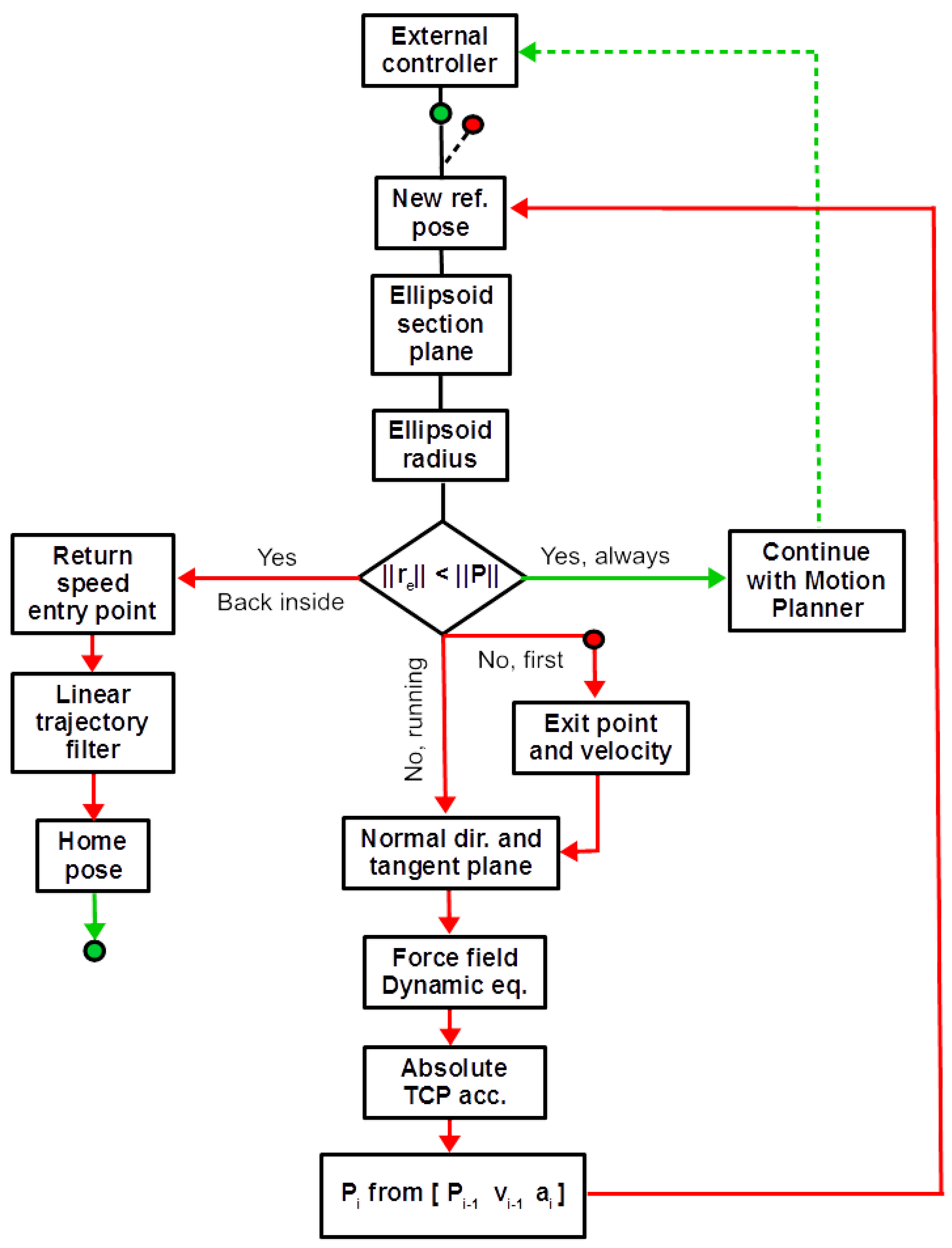
3.4. Workspace Safety Algorithm

At middle level, the output pose from trajectory planner is managed by means of cyclic buffering technique. A write index (W) and a read index (R) are updated each control cycle and used to access the buffer. Time-base control, whose specific functioning is not a topic of this article, works to maintain the distance between R and W at a default value, slightly altering velocity for small move sections. The objectives of this routine are to always have at least one reference point ahead, to work most of the time in the minimum delay default condition, using the smallest effective distortion to restore default indexes distance when necessary. This method gives the opportunity to calculate high quality smooth trajectories, even for our case in which future external loads and therefore future references are hardly predictable, and remedying finite CPU clock resolution that affects every timing routine. Moreover, buffering technique offers the opportunity to look for future violation of WS limits.

The lowest level of the Motion-Planner is occupied by the routines that transform TCP workspace references into actuators workspace setpoints. Among all, consecutive moves blending, trajectory segmentation, inverse kinematics computation and high frequency interpolation at actuators level.

As mentioned above, it is required to avoid dynamic shocks of the turbine base to prevent possible dangerous situations. For this reason, it is not convenient to use the ellipsoid limit obtained as a simple saturation surface: this would cause severe deceleration, especially during high velocity saturation reaching. The algorithm implemented, instead, use this surface as a soft/compliant limit. The main purpose is to avoid uncontrolled references to be commanded outside robot optimum performances volume, but without introducing discontinuities in the velocity profile of the TCP and controlling the acceleration imposed on the turbine. This requirement is fulfilled by modeling the dynamic behaviour of the TCP interacting with the virtual compliant limit, so that it will act conveniently on the tangential and orthogonal direction with respect to ellipsoid surface. This approach is considerable as a particular haptic case of interaction with virtual environment [24]. However, some considerations about this assumption are necessary: since the workspace constraint formulation is based on robot optimum manipulation capabilities, exceeding application specific range of expected motion, we are not interested in keeping a steady or dynamic operative condition outside the computed limit. The algorithm proposed has to be primary intended as an emergency control logic, whose goal is to restore normal and controlled operative conditions in presence of unwanted/unexpected behaviour of the HIL system, whose normal expected behaviour is well inside the limits formulated. The haptic concept of equivalent mechanical system emulation during contact with virtual objects, is used here in order to obtain a continuous and stable deflection of TCP trajectory, but we are not interested in keeping active the force feedback loop once outside the limit. The reason behind this choice is that the HIL setup proposed is intended to be used like a realistic source of operative condition for monitoring scaled wind turbine behaviour: any force source not intended to be a scaled reproduction of some real effect could make tests ineffective. The main steps of the procedure are summarized in Figure 9.

A hard limit is fixed, for additional safety, by expanding the ellipsoid. The expansion coefficient is calculated so that the new surface remains within a new total-orientation WS obtained with less restrictive multiplication of external loads constraint. The three surfaces are shown in Figure 10. This external surface is used as a simple limit that puts the robot in the error state and stops any test and motion. This is to have a blended and controlled stop in the case of any other software safety algorithm failure, including the one described here, acting before software limits on the sliders and hardware limits.

For every move time cycle, a new global reference pose hase to be written in the buffer, represented inside Motion Planner scheme in Figure 8; the actual TCP commanded position $\mathbf{P}={\left\{P_x{P}_y{P}_z\right\}}^T$, expressed in the nominal WS centred frame, is extracted from the new reference pose together with its magnitude. Referring to Figure 6, the parameter $\phi$ is calculated as follows:

$$\phi =arctan\left(\frac{P_y}{P_x}\right)$$

(5)

while, to calculate the value of $\theta$, it is necessary to consider the projection of vector $\mathbf{P}$ along the local ${\widehat{\mathbf{x}}}_{\mathbf{l}}$ axis. The value of $P_{xl}$ is equal to:

$$P_{xl}=\mathrm{sign}(P_x)\sqrt{P_x^2+P_y^2}$$

(6)

and the value of $\theta$ can be obtained as:

$$\theta =arctan\left(\frac{P_z}{P_{xl}}\right)$$

(7)

Every case involving degeneration to zero of one or more components of $\mathbf{P}$ is treated separately, so that continuous results on $\phi$ and $\theta$ are guaranteed. From $\phi$ and $\theta$, the corresponding value of ${\mathbf{r}}_{\mathbf{e}}$ is calculated; it constitutes the radius of the internal ellipsoid along the direction of the position vector $\mathbf{P}$. If the magnitude of $\mathbf{P}$ is inferior to the one of ${\mathbf{r}}_{\mathbf{e}}$, then the TCP is still commanded to stay inside internal ellipsoid and no further actions are necessary. The reference read from the buffer is left unchanged and processed by subsequent algorithms of the Motion Planner.

Otherwise, if $\left|\right|{\mathbf{r}}_{\mathbf{e}}\left|\right|<\left|\right|\mathbf{P}\left|\right|$, a command outside the limit is detected. This condition is considered dangerous due to insufficient robot performances outside the hard limit, according to boundary conditions used during limit surface formulation. Moreover, a reference pose, given by the dynamic model of the floating substructure, outside nominal workspace, is indicative of a model unpredicted/unwanted behaviour that is necessary to control before possibly dangerous pose is commanded to the robot. Since the internal ellipsoid surface is already a permissive limit compared to the nominal workspace, once it has been violated is necessary that safety algorithm takes control of the new reference generation process, no more belonging to dynamic model integration. The external dSPACE controller, dealing with robot reference poses computation, is warned by a status flag about Power PMAC mastering reference generation process. The first commanded pose outside the limits, from now on called ${\mathbf{P}}_{\mathbf{0}}$, is used to compute algorithm’s initial conditions, such as exit velocity magnitude and direction.

Two other unitary vectors are computed, representing two ellipsoid tangent directions with respect to point ${\mathbf{r}}_{\mathbf{e}}$, identifying the tangent plane. The cartesian components of the tangent vectors ${\mathbf{t}}_{\theta }$ and ${\mathbf{t}}_{\phi }$ can be expressed taking the partial derivatives of the ellipsoid cartesian coordinates in Equation (4) with respect to $\theta$ and $\phi$. The unitary vectors are then obtained by dividing both $\mathbf{t}$ for its correspondent norm. Thanks to these two unitary vectors, it is possible to calculate the normal unitary vector ${\widehat{\mathbf{n}}}_e$ of the tangent plane, such that it points always outside the ellipsoid surface:

$$\begin{array}{cc}\hfill {\widehat{\mathbf{n}}}_{\mathbf{e}}& ={\widehat{\mathbf{t}}}_{\theta }\times {\widehat{\mathbf{t}}}_{\phi }\mathrm{if}\frac{\pi }{2}\le \theta \le \frac{3}{2}\pi \hfill \end{array}$$

(8)

$$\begin{array}{cc}\hfill {\widehat{\mathbf{n}}}_{\mathbf{e}}& ={\widehat{\mathbf{t}}}_{\phi }\times {\widehat{\mathbf{t}}}_{\theta }\mathrm{if}-\frac{\pi }{2}\le \theta \le \frac{\pi }{2}\hfill \end{array}$$

(9)

The exit velocity vector ${\mathbf{v}}_{\mathbf{0}}={\left\{v_{0x}{v}_{0y}{v}_{0z}\right\}}^T$ is calculated through the incremental ratio of each component of command position ${\mathbf{P}}_{\mathbf{0}}$ with respect to numeric computed actual TCP position vector. The component of this vector along the normal direction on the ellipsoid surface is calculated as:

$$v_n=\mathbf{v}·{\widehat{\mathbf{n}}}_{\mathbf{e}}$$

(10)

and the tangential velocity vector is obtained as:

$$\begin{array}{c}\hfill {\mathbf{v}}_t=\mathbf{v}-v_n{\widehat{\mathbf{n}}}_{\mathbf{e}}\\ \hfill {\widehat{\mathbf{n}}}_{\mathbf{t}}=\frac{{\mathbf{v}}_t}{\left|\right|{\mathbf{v}}_t\left|\right|}\end{array}$$

This vector lies in the tangential plane identified by ${\mathbf{t}}_{\theta }$ and ${\mathbf{t}}_{\phi }$. At this point, the algorithm deflects the TCP velocity maintaining continuity. To do that, two dynamic systems are implemented, acting every cycle on the fresh computed normal and tangential direction. The effects desired is equivalent to that of a viscous environment on tangential directions and viscoelastic on normal directions, imposing a dissipative force field on the TCP, considered as a concentrated mass, once outside internal surface. Initial position and velocity are modified every cycle applying the resulting acceleration, computed by dynamic equilibrium of the forces applied on the TCP.

The magnitude of the normal acceleration to be applied is equal to:

$$a_n=c_{n,eq}{v}_n+k_{n,eq}\Delta r_n$$

(11)

where $c_{n,eq}$ is an equivalent damping coefficient in the normal direction, $k_{n,eq}$ is an equivalent normal spring stiffness and $\Delta r_n$ is the component on the normal direction of the difference between $\mathbf{P}$ and ${\mathbf{r}}_e$, assuming that the relaxed position of the normal spring lies on the surface. The vectorial acceleration in normal direction is:

$${\mathbf{a}}_n=-a_n{\widehat{\mathbf{n}}}_{\mathbf{e}}$$

(12)

In the same way, the magnitude of the acceleration along the tangential direction is:

$$a_t=c_{t,eq}{v}_t$$

(13)

where $c_{t,eq}$ is the equivalent damping coefficient of the damper applied in tangential direction, and the vectorial form of the tangential acceleration is:

$${\mathbf{a}}_t=-a_t{\widehat{\mathbf{n}}}_{\mathbf{t}}$$

(14)

The two accelerations are combined to get the total acceleration vector to be applied:

$${\mathbf{a}}_{tot}={\mathbf{a}}_t+{\mathbf{a}}_n$$

(15)

thanks to which, the new commanded position of the TCP ,expressed in the reference frame positioned in the workspace centre, is calculated as:

$${\mathbf{P}}_{\mathbf{1}}={\mathbf{P}}_{\mathbf{0}}+{\mathbf{v}}_{\mathbf{0}}\Delta t+\frac{1}{2}{\mathbf{a}}_{tot}\Delta t^2$$

(16)

In each new cycle, a new point of the modified time history of ${\mathbf{P}}_{\mathbf{i}}$ is computed, starting from ${\mathbf{P}}_{\mathbf{i}-\mathbf{1}}$, ${\mathbf{v}}_{\mathbf{i}-\mathbf{1}}$, ${\mathbf{a}}_{\mathbf{i}}$ and all the ellipsoid parameters relative to the last position ${\mathbf{P}}_{\mathbf{i}-\mathbf{1}}$. The initial normal component of the velocity is gradually dissipated until the elastic action cause the normal acceleration inversion and the TCP is attracted back towards the ellipsoid limit. Instead, the tangent component of the velocity cause the TCP to travel between the internal and external ellipsoid and the normal direction to be recomputed each cycle. The viscous effect gradually reduces $v_t$, so that TCP absolute velocity becomes gradually normal to the ellipsoid surface and the elastic action exerted on this direction ensures the return back inside internal ellipsoid. The trajectory followed by the TCP depends on:

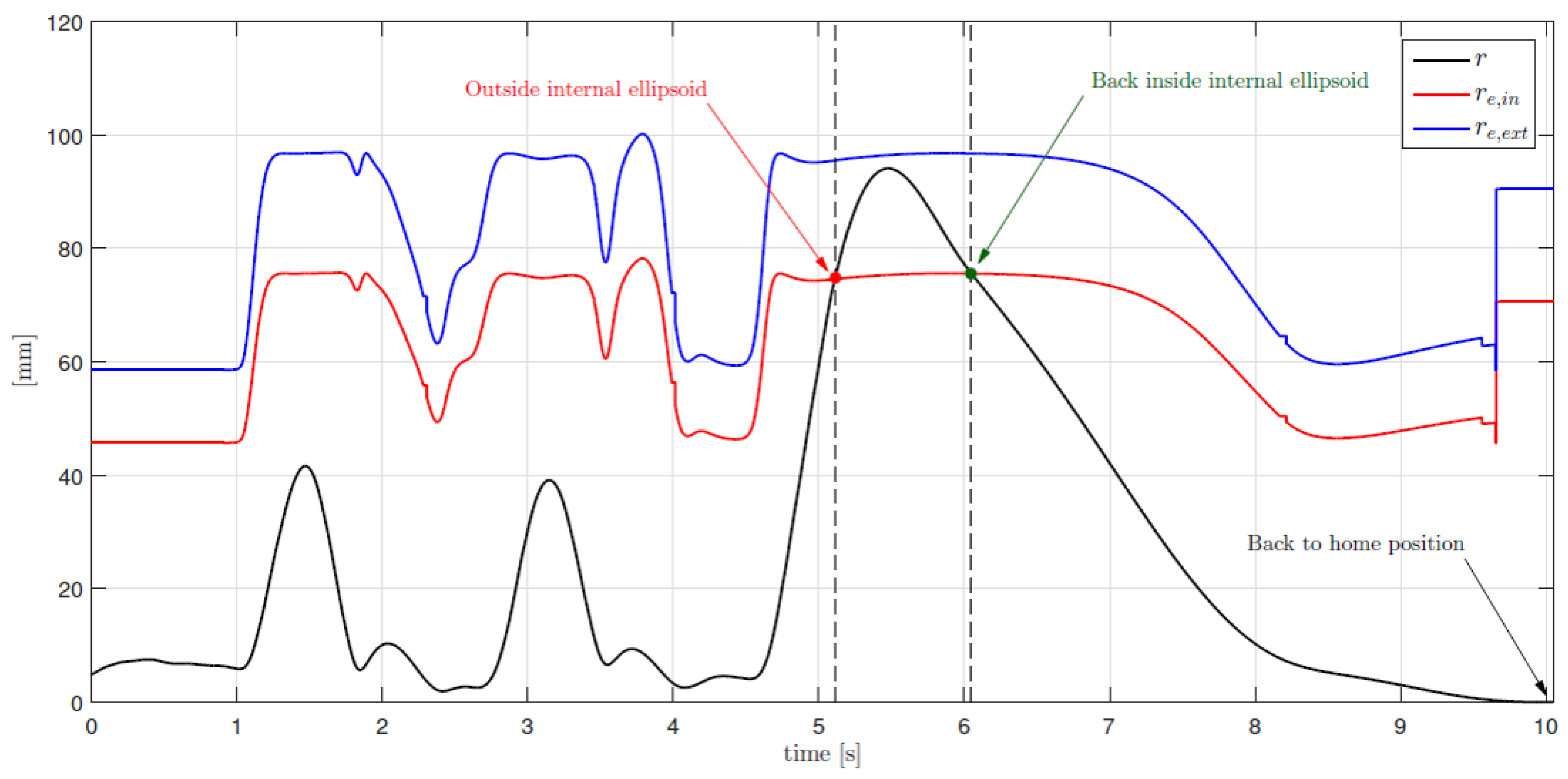
• Exit velocity magnitude and direction.
• Ellipsoid shape near the exit point; velocity components on normal and tangent direction evolve influenced even by ellipsoid shape found during trajectory progression.
• Dynamic parameters of the compliant limit.

Dynamic parameters tuning of the compliant limit allows respecting the limits set on TCP maximum acceleration. Velocity gradual alignment on normal direction not only guarantee TCP return inside the limit, but also prevent an immediate new exit once back inside the surface, possible if the return inside point is placed in a severe curvature region of the surface and the re-entry velocity has a relevant component along major curvature direction. During this procedure, the orientation of the TCP is kept constant to the exit condition.

Once back inside the safety limit, the robot is brought back to home position with zero orientation to restart the test and give back the reference generation charge to the dynamic model integrator dealing with the force loop. This is done again preserving velocity continuity: once back inside the ellipsoid, the force field is turned off, the undisturbed linear trajectory, resulting from keeping constant the re-entry velocity, is filtered through a ramp coefficient going from 1 to 0, so that the home pose is smoothly restored without introducing discontinuities.

4. Simulation

In the following section, simulation results of this algorithm is provided. A simulation scheme has been developed in Matlab/Simulink environment to verify the correct functioning of the algorithm steps: a simple sinusoidal motion reference for the TCP is used as input, written in the local $XY$ plane corresponding to local Z equal to zero and global Z equal to homing height $Z_{wsd}$. The results refer to the standalone implementation of the specific Motion Planner section dealing with workspace boundaries safety algorithm.

In Figure 11, the entire simulation is provided: looking at Figure 11a, the intersection between the sinusoid and the red dotted line, represent the first exit point of the TCP outside the soft limit. The red dotted line, visible as a dotted shape in the other sub-figures, represent the ellipsoid shape at the $\phi$ section containing the exit point. Once outside the limit, the sinusoid reference is ignored and the modified trajectory in solid red is computed: looking at all the different view angles provided, it is visible how the red trajectory bend in all three directions is influenced by the ellipsoid shape and by the exit velocity direction and modulus, preserving continuity with the exit velocity at the beginning of the trajectory. The intersection between modified trajectory in red and the grey dotted line in Figure 11a represents the return back inside point in the ellipsoid. As said before, all the other grey dotted shapes shown in the other sub-figures represent different view angles of the ellipsoid section containing the return point. Once back inside the limit, the TCP is brought back to nominal workspace origin, corresponding to home position. Once again, it is clear how velocity continuity is preserved during the outside/inside limit transition and approaching the final pose.

5. Experimental Results

The implementation of the described algorithm has been carried out on the Power PMAC motion controller, together with all the other control stages apart from motors torque loop and phase commutation. The WS boundaries safety algorithm is implemented at high level, among the group of routines part of Motion Planner architecture, as shown in Figure 8. In particular, this safety stage is positioned immediately after analog reference sampling, coming from dSPACE controller, dealing with floater/sea dynamic model integration. Each new reference is analysed and eventually modified by three routines, identified by the Trajectory Planner box in Figure 8; once the new reference has been processed, it is then inserted in the reference buffer according to current write-index position. The specific code associated with WS boundaries check algorithm is implemented in two main sections: the first is basically a small state machine, written in Omron Delta Tau script language inside a PLC program, dealing with logic distinction between all the different operative conditions of the safety routine and the corresponding effect desired on the main robot state machine; and, the second, written in C language to improve computation speed, is called by the state machine and deals with all ellipsoid computations and trajectory modification.

A test has been conducted on the 1:3 scaled version of the robot shown in Figure 12, using the Position Based Admittance Control (PBAC); this control mode allows emulating exactly the operative control mode that will be exploited inside wind tunnel, apart from the fact that the dynamic model used is way simpler than the real one and run directly by the motion controller. Actual testing has been carried out with Motion Planner architecture functioning at 0.4 kHz at high level and 1.6 kHz at low level, corresponding to 2.5 ms end-effector references computation and 0.625 ms motors references computation. Real-time pose estimation is performed at 1.6 kHz. The input force is provided through a joystick installed on a six axis ATI mini45 F/T sensor, instead of using wind action on the turbine as loads input. The robot platform is commanded to emulate the dynamic behaviour of a simple spherical mass with six independent degrees of freedom, connected to the environment with six spring-dampers on its COG, three acting on translations and three on rotations. Dynamics coefficient are setto match natural frequencies on every DOF, convenient dimensionless damping coefficients and static spring elongation compatible with external loads exerted by hands. Hexafloat and control capabilities about dynamic model emulation and perceived transparency, are not topics of this article and are discussed in another work.

During a random load exerted on the joystick, the robot end-effector is voluntarily pushed outside the limit for testing the safety algorithm. All the time histories reported refer to real-time robot pose, estimated through numeric solution of the nonlinear forward kinematics equations.

Looking at Figure 13, the two dotted black lines identify the exit and return back instants. The robot is kept between internal and external limits during the procedure. The red and blue curves represent the time history of both internal and external ellipsoid radius computed each cycle on the same direction of r. In Figure 14, the complete time history of the TCP position is provided, showing the algorithm effectiveness about preserving velocity continuity during all the procedure. Finally, Figure 15 shows the time history of the TCP orientation, represented by the three Euler angles $\alpha ,\beta ,\gamma$. As described in Section 3.4, the orientation is kept unchanged during the time spent by the TCP between the two limit surfaces; once back inside, all three angles are brought back to zero, always preserving continuity.

6. Conclusions

The characteristic workspace limiting requirements coming from the LIFES50+ project have been discussed. An efficient strategy for limiting the operative workspace of a six DOF PKM robot carrying high inertia objects is described and experimental results are provided. The safety algorithm presented is capable of realizing a virtual compliant surface, exerting on the robot a variable force field dependent on TCP absolute position and velocity between two control surfaces. Velocity magnitude and direction continuity are efficiently preserved, preventing dangerous vibrations triggered by simple and abrupt saturations arranged in the TCP domain. The results show optimum and efficient behaviour satisfying the imposed requirements, well integrated with the overall control of the robot. Thanks to efficient control threads priority managements, this safety routine does not have any additional influence in terms of delay and tracking error while inside the internal surface with respect to performance imposed by the buffering technique. The scaled robot allows us to efficiently verify and optimize this and other control routines that will be implemented on the full scale machine.

Additional verifications and fine tuning will be carried out on the full scale robot. As described in Section 3.4, while for the HIL tests planned we are not interested in keeping active the force feedback loop once outside the limit surface, further development of this work will include this possibility. In particular, future studies will focus on active regulation of the operative conditions of the test, giving the possibility to vary wind velocity and turbulence. In this scenario, the dynamic six DOF weight scale installed on the TCP, once outside the limit surface, will keep the force feedback loop active, taking into consideration aerodynamic and hydrodynamic loads cooperating with the force field caused by modelled environment impedance. The safety algorithm presented is designed so that this new condition can be realized by simply adding measured force to presently used dynamic six DOF weight scale and using real time estimated pose to track the modified dynamic behaviour of the system.

References

- Bayati, I.; Belloli, M.; Bernini, L.; Fiore, E.; Giberti, H.; Zasso, A. On the functional design of the DTU10 MW wind turbine scale model of LIFES50+ project. J. Phys. 2016, 753, 052018. [Google Scholar] [CrossRef]
- Bak, C.; Zahle, F.; Bitsche, R.; Kim, T.; Yde, A.; Henriksen, L.C.; Hansen, M.H.; Blasques, J.P.A.A.; Gaunaa, M.; Natarajan, A. The DTU 10-MW reference wind turbine. In Danish Wind Power Research 2013; Technical University of Denmark: Kongens Lyngby, Denmark, 2013. [Google Scholar]
- Fathy, H.K.; Filipi, Z.S.; Hagena, J.; Stein, J.L. Review of hardware-in-the-loop simulation and its prospects in the automotive area. Ann. Arbor. 2006, 6228, 62280E-1. [Google Scholar]
- Carignan, C.; Scott, N.; Roderick, S. Hardware-in-the-loop simulation of satellite capture on a ground-based robotic testbed. In Proceedings of the 12th International Symposium on Artificial Intelligence, Robotics and Automation in Space (iSAIRAS), Montreal, QC, Canada, 17–19 June 2014. [Google Scholar]
- Isermann, R.; Schaffnit, J.; Sinsel, S. Hardware-in-the-loop simulation for the design and testing of engine-control systems. Control Eng. Pract. 1999, 7, 643–653. [Google Scholar] [CrossRef]
- Brünger-Koch, M. Motion parameter tuning and evaluation for the DLR automotive simulator. In Proceedings of the 2005 Driving Simulator Conference (DSC NA CD-ROM), Orlando, FL, USA, 30 November–2 December 2005. [Google Scholar]
- Giberti, H.; Ferrari, D. A novel hardware-in-the-loop device for floating offshore wind turbines and sailing boats. Mech. Mach. Theory 2015, 85, 82–105. [Google Scholar] [CrossRef]
- Bayati, I.; Belloli, M.; Facchinetti, A.; Giappino, S. Wind tunnel tests on floating offshore wind turbines: A proposal for hardware-in-the-loop approach to validate numerical codes. Wind Eng. 2013, 37, 557–568. [Google Scholar] [CrossRef]
- D’Antona, G.; Davoudi, M.; Ferrero, R.; Giberti, H. A model predictive protection system for actuators placed in hostile environments. In Proceedings of the 2010 IEEE International Instrumentation and Measurement Technology Conference (I2MTC 2010), Austin, TX, USA, 3–6 May 2010; pp. 1602–1606. [Google Scholar]
- Bayati, I.; Belloli, M.; Ferrari, D.; Fossati, F.; Giberti, H. Design of a 6-DoF robotic platform for wind tunnel tests of floating wind turbines. Energy Procedia 2014, 53, 313–323. [Google Scholar] [CrossRef]
- Fiore, E.; Giberti, H. Optimization and comparison between two 6-DoF parallel kinematic machines for HIL simulations in wind tunnel. In Proceedings of the MATEC Web of Conferences, Singapore, Singapore, 13–14 January 2016; Volume 45. [Google Scholar]
- Ferrari, D.; Giberti, H. A genetic algorithm approach to the kinematic synthesis of a 6-DoF parallel manipulator. In Proceedings of the 2014 IEEE Conference on Control Applications (CCA 2014), Juan Les Antibes, France, 8–10 October 2014; pp. 222–227. [Google Scholar]
- Giberti, H.; Ferrari, D. Drive system sizing of a 6-DOF parallel robotic platform. In Proceedings of the ASME 12th Biennial Conference on Engineering Systems Design and Analysis (ESDA 2014), Copenhagen, Denmark, 25–27 July 2014; Volume 3. [Google Scholar]
- Fiore, E.; Giberti, H.; Ferrari, D. Dynamics modeling and accuracy evaluation of a 6-DoF hHexafloat robot. In Nonlinear Dynamics; Springer: Berlin/Heidelberg, Germany, 2016; Volume 1, pp. 473–479. [Google Scholar]
- Fiore, E.; Giberti, H.; Bonomi, G. An innovative method for sizing actuating systems of manipulators with generic tasks. Mech. Mach. Sci. 2017, 47, 297–305. [Google Scholar]
- Bonev, I.A.; Ryu, J. A geometrical method for computing the constant-orientation workspace of 6-RRS parallel manipulators. Mech. Mach. Theory 2001, 36, 1–13. [Google Scholar] [CrossRef]
- Merlet, J.P. Determination of 6D workspaces of Gough-type parallel manipulator and comparison between different geometries. Int. J. Robot. Res. 1999, 18, 902–916. [Google Scholar] [CrossRef]
- Gosselin, C. Determination of the workspace of 6-dof parallel manipulators. ASME J. Mech. Des. 1990, 112, 331–336. [Google Scholar] [CrossRef]
- Kim, D.; Chung, W.K.; Youm, Y. Geometrical approach for the workspace of 6-dof parallel manipulators. In Proceedings of the 1997 IEEE International Conference on Robotics and Automation, Albuquerque, NM, USA, 25 April 1997; Volume 4, pp. 2986–2991. [Google Scholar]
- Cao, Y.; Huang, Z.; Zhou, H.; Ji, W. Orientation workspace analysis of a special class of the Stewart–Gough parallel manipulators. Robotica 2010, 28, 989–1000. [Google Scholar] [CrossRef]
- Bonev, I.A.; Ryu, J. A new approach to orientation workspace analysis of 6-DOF parallel manipulators. Mech. Mach. Theory 2001, 36, 15–28. [Google Scholar] [CrossRef]
- Shen, G.; Tang, Y.; Zhao, J.; Lu, H.; Li, X.; Li, G. Jacobian free monotonic descent algorithm for forward kinematics of spatial parallel manipulator. Adv. Mech. Eng. 2016, 8. [Google Scholar] [CrossRef]
- La Mura, F.; Todeschini, G.; Giberti, H. High Performance Motion-Planner Architecture for Hardware-In-the-Loop System Based on Position-Based-Admittance-Control. Robotics 2018, 7, 8. [Google Scholar] [CrossRef]
- Adams, R.J.; Hannaford, B. Stable haptic interaction with virtual environments. IEEE Trans. Robot. Autom. 1999, 15, 465–474. [Google Scholar] [CrossRef]