Abstract
The presented work is part of the H2020 project SWEEPER with the overall goal to develop a sweet pepper harvesting robot for use in greenhouses. As part of the solution, visual servoing is used to direct the manipulator towards the fruit. This requires accurate and stable fruit detection based on video images. To segment an image into background and foreground, thresholding techniques are commonly used. The varying illumination conditions in the unstructured greenhouse environment often cause shadows and overexposure. Furthermore, the color of the fruits to be harvested varies over the season. All this makes it sub-optimal to use fixed pre-selected thresholds. In this paper we suggest an adaptive image-dependent thresholding method. A variant of reinforcement learning (RL) is used with a reward function that computes the similarity between the segmented image and the labeled image to give feedback for action selection. The RL-based approach requires less computational resources than exhaustive search, which is used as a benchmark, and results in higher performance compared to a Lipschitzian based optimization approach. The proposed method also requires fewer labeled images compared to other methods. Several exploration-exploitation strategies are compared, and the results indicate that the Decaying Epsilon-Greedy algorithm gives highest performance for this task. The highest performance with the Epsilon-Greedy algorithm ( = 0.7) reached 87% of the performance achieved by exhaustive search, with 50% fewer iterations than the benchmark. The performance increased to 91.5% using Decaying Epsilon-Greedy algorithm, with 73% less number of iterations than the benchmark.
1. Introduction
Agricultural robots exist to perform a variety of tasks, such as harvesting, trimming, transplanting and cultivating. Recently, a lot of research has been done on harvesting robots due to the lack of skilled workforce to do manual harvesting and an increase in salaries [1].
The EU H2020 project SWEEPER (G.A. 644313) (http://www.sweeper-robot.eu) [2,3,4] aims at brining the first generation of sweet pepper harvesting robots onto the market. Due to the dynamic and unstructured nature of greenhouse environment, the fruit detection part is very challenging. Several types of sensors and methods are suggested, see [5,6] for reviews. This paper proposes a new approach for yellow pepper detection from images of greenhouse environments. The proposed approach does not suffer from subjective tuning of parameters, and can therefore be used also in other application domains involving dynamic environments. In the SWEEPER project the developed method is intended to be used to detect sweet pepper fruits and to guide the arm towards the fruit using visual servoing. Figure 1 shows a block diagram of how this work fits into the developed robotic harvesting system. A pepper detection module outputs the location of all detected fruits in image coordinates to the visual servoing routine, which selects one of the fruits and computes the Δpose required to move the selected fruit to the center of the camera image. This value is added to the current pose and sent to a motion planner that guides the arm to the desired position.
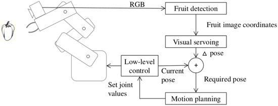
Figure 1.
The developed image segmentation technique is designed to be part of a robotic system that guides the robotic manipulator towards a detected fruit using visual servoing.
Despite intense research on harvesting robots and recent improvements, the performance of these robots are not sufficient compared to manual harvesting [7]. For fruit harvesting robots, one bottleneck is the fruit detection algorithms; Bac et al. [8] reported state of the art detection rate being 85% in their 2014 review. Fruit detection is a complex task due to the demanding agricultural environmental conditions. Different light conditions, unstructured and dynamic surrounding environments, and occlusions significantly affect the performance of detection algorithms. Image segmentation is one of the most difficult low-level image analysis tasks [9,10] and a critical step in many computer vision operations, such as feature extraction, object detection, and recognition. The main objective of segmentation is separating background and foreground to extract the regions of interest in the image. Despite the variety of existing methods for image segmentation with promising performance, it is still not proven that these methods can be used in diverse applications [11]. In these methods, the key parameters are manually tuned by system designers using trial and errors approaches, and the parameters cannot be adapted to environmental changes. Therefore, changes of the environmental conditions result in degraded performance. Shadows, light intensity and occlusions are some sources of changes in the environment.
A common method for segmentation is image thresholding. Considering the unstructured environment in a greenhouse and that the background and foreground features are similar, it is challenging to find the optimal threshold. Literature in computer vision demonstrate that pre-selected thresholds fail to correctly segment the image in most applications [10,12]. Therefore, adaptive thresholding has been used in many vision based agricultural applications, where the threshold is changed adaptively based on illumination conditions [13,14,15].
This paper introduces a novel method for a global adaptive image thresholding based on reinforcement learning (RL). Recently, RL has been used for a variety of image processing tasks such as image thresholding and object recognition. RL is based on interaction with the environment and analysis of a received numerical reward signal. It is different from supervised learning, which uses training examples provided by an expert supervisor. In many applications it is not possible to get enough examples to cover the entire parameter space, and it is more beneficial to learn from experience.
Shokri and Tizhoosh [16] trained an RL agent to learn the optimal weights of thresholds delivered by several thresholding algorithms, and use the fused thresholds to segment the image. Bhanu and Peng [17] introduced an image segmentation method that learns segmentation parameters using connectionist reinforcement learning technique based on environmental conditions. Peng and Bhanu [18] also used RL to create a mapping from input images to the parameters used for the segmentation of corresponding images in training step. An RL agent was trained for threshold tuning by Sahba and colleagues [19]. Additionally, RL has been used for maximum entropy thresholding, with reduced computational concerns [20]. Moreover, it is shown that it is beneficial to use RL for classification of objects [18,21]. Reinforcement learning has also been used in many other applications, such as web applications [22,23], control and management problems [24,25], and also in grid and cloud computing [26,27].
The rest of this paper is organized as follows: Section 2 summarizes image thresholding and segmentation quality measures; In Section 3 the proposed method is described; In Section 4 training and testing procedures are discussed and the experimental results are presented in Section 5; Conclusions and future work are presented in Section 6.
2. Image Thresholding
The goal of image segmentation is to divide an image into multiple segments in order to simplify further image analysis such as feature extraction, object detection and object recognition. One of the most common segmentation methods is thresholding, which splits an image into foreground and background [28,29,30] where the foreground contains the object of interest. A common thresholding technique is to first convert the RGB image to HSI or HSV color space [28] and then perform thresholding [31,32]. This decreases the effect of illumination changes in the image. A lower and upper threshold, different for hue and saturation images, determine which pixels are considered as background or foreground. A pixels is regarded as foreground if it is within the threshold window of both hue and saturation.
In this work, we use an RL-based technique to adaptively find thresholds for hue and saturation images such that it results in an optimally segmented image.
2.1. Segmentation Quality
A critical part in RL is the reward function, which in our case reflects the segmentation quality. To compute segmentation quality, two measures are introduced [33]: segmentation-overlap and segmentation-efficiency as illustrated in Figure 2. Segmentation-overlap is defined as the ratio between the number of pixels in the overlapped region (A) (i.e., pixels common to the segmented region (D) and the labeled region (E)) and the total number of pixels in the labeled region (E). It indicates how large area of the labeled pepper is segmented. For example, if the segmentation overlap is 0.9, then 90% of the pixels labeled as pepper are also segmented. Segmentation-efficiency is defined as the ratio between the number of pixels in the overlapped region (A) and the total number of pixels in the segmented area (D). It indicates how large part of the segmented area is labeled as pepper. For example, if the segmentation-efficiency is 0.8, then 20% of the segmented region covers the background and not the pepper. The performance measurements are within the range [0, 1]. The average of segmentation-overlap and segmentation-efficiency is used as a measure of segmentation quality q:

Figure 2.
Segmentation-overlap and segmentation-efficiency is used to compute segmentation quality.
The highest segmentation quality is achieved where both segmentation-overlap and segmentation-efficiency are 1, meaning segmented and labeled regions overlapped completely. High segmentation-overlap and low segmentation efficiency means that the segmented region covers a large part of the pepper, while only a small part of the segmented region contains parts of the pepper. Low segmentation-overlap and high segmentation-efficiency means that that the segmented region covers only a small part of the pepper, while a large part of the segmented region contains parts of the pepper.
3. Reinforcement Learning-Based Thresholding
A straightforward method to achieve optimal thresholds is to use trial and error. That is, testing different thresholds until the objective level of similarity between segmented image and labeled image is achieved. A problem with this is that it uses an excessive amount of computational resources [18]. Using reinforcement learning can speed up the process of finding the optimal threshold. Reinforcement learning (RL) works through iterative interactions with the environment based on trial and error [34]. In RL, the learning environment is formulated as a Markov Decision Process (MDP) described by a tuple where S is the set of environment states, A is the set of possible actions, T is the transition function specifying the transition probability of each state s by taking action a, and R is reward function which defines the reward of transition from state s to a new state by taking action a.
In this work Q-learning [34], a well-known algorithm in the class of Temporal Difference, was chosen to be applied to the problem of adaptive image thresholding.
Since in this work transition and reward function are non-deterministic, it is essential to represent the environment in a non-deterministic way. The agent updates state-action values in a non-deterministic environment as follows:
where is the learning rate and is the learned state-action value for a given state and action at time t. is the discount factor that defines the importance of future rewards and r is the reward value. If the discount factor is set to 0 the agent only considers the immediate reward, while if the value approaches 1, the agent focus on the long term reward.
Equation (3) defines the learning rate ( in Equation (2)) in a non-deterministic environment [35] where is the total number of times the tuple has been visited. Using Equations (2) and (3), updates of Q-values are made more gradually than in the deterministic case [35]. If the value of in Equation (2) is set to 1 it would be a deterministic case. The value in Equation (3) reduces as n increases, therefore, update values get smaller as training continues.
In the proposed method for image thresholding, given an image, the transition function does not give a new state but instead output a new form of the image. This is motivated by the n-armed bandit problem [34]. In this framework, the current state in Q-table is affected only by the previous visits of this state (first order MDP). Therefore, Equation (2) is modified as:
In the rest of this section we describe our approach based on reinforcement learning for image thresholding.
3.1. Proposed Algorithm
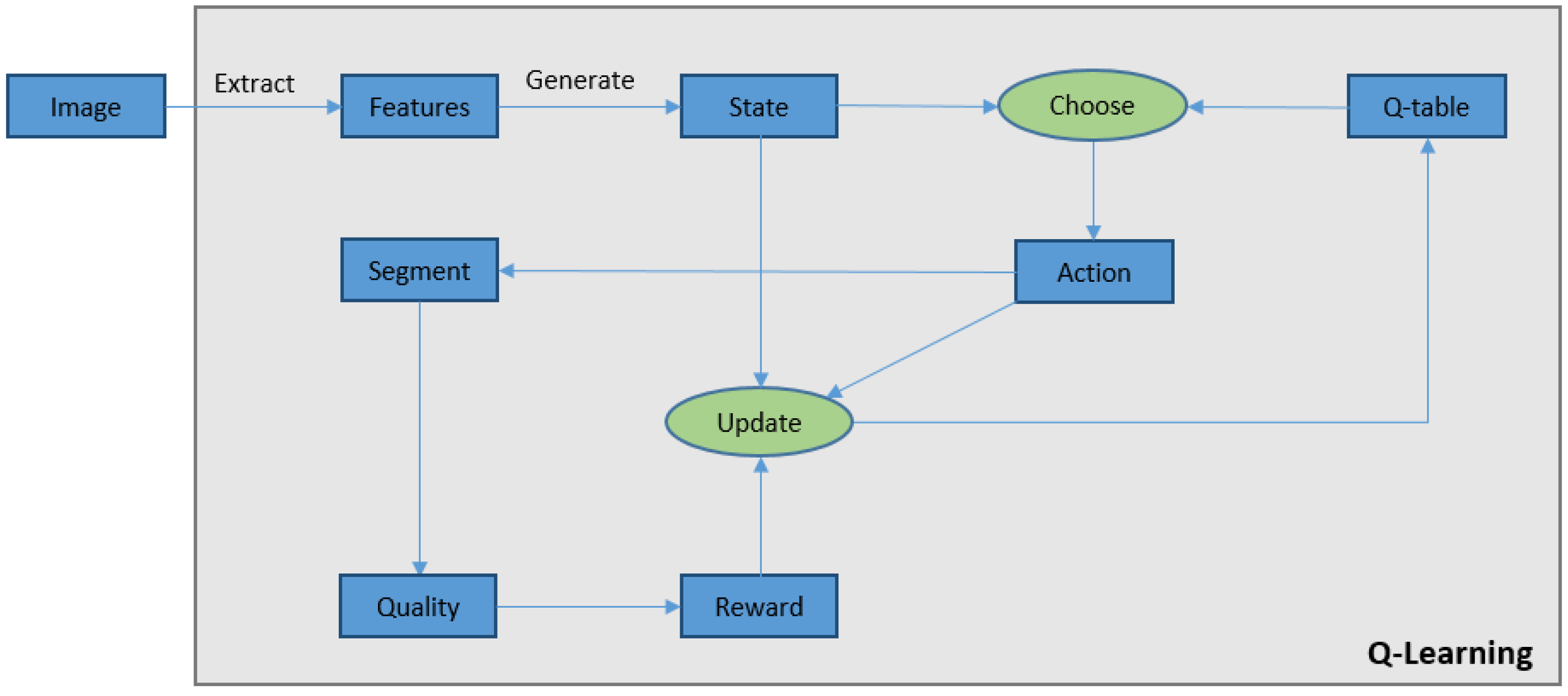
The pseudo-code of the method is presented in Figure 3. In this approach, for each input image, initially hue and saturation features are extracted to find the state of the image. Then, an action (threshold) is selected and applied to the image to segment it. The process followed by comparing the segmented image with the ground truth (labeled image) to measure the segmentation quality. The quality measure q (Equation (1)) is used as a reward function to update the Q-table using Equation (4). The whole process continues until it reaches the convergence condition (Equation (8)). The structure of the proposed approach is also illustrated in Figure 4.
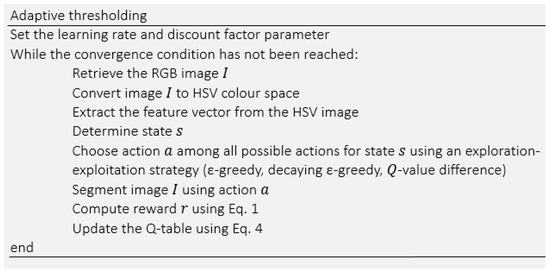
Figure 3.
The proposed approach for adaptive image thresholding based on reinforcement learning (RL).
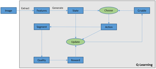
Figure 4.
Illustration of the proposed algorithm for image segmentation using Q-learning. For each image the state is determined and an action is selected to segment the image. Then the segmentation quality function is used to compare the segmented image with the ground truth to compute the reward and update the Q-table.
3.2. Image thresholding as an MDP
The tuple elements of the MDP are described as follows in our approach.
3.2.1. States
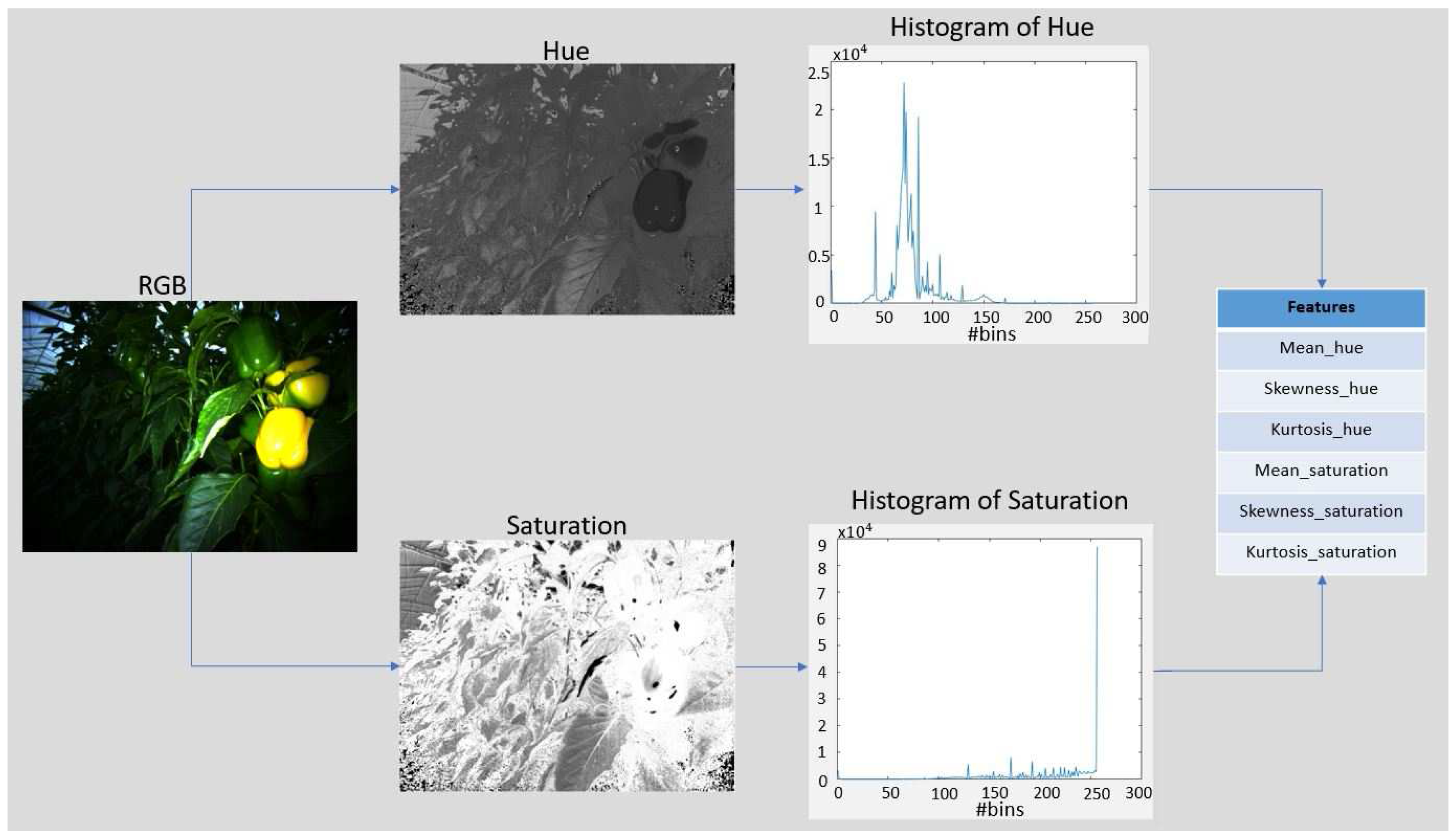
In this work, states are the representations of images. There are different methods of defining states using various image features. We converted the RGB image to HSV color-space, and then features are extracted from hue H and saturation S histograms. Extracted features include mean m, skewness s and kurtosis k of both H and S. The result is a feature vector of 6 dimensions which can highly discriminate between images. The method used for feature extraction is shown in Figure 5. We used a k-means clustering algorithm on the values of each feature in the feature vectors and extracted centroids of feature clusters [18]. The state of MDP is defined by a 6-tuples where each element is the value of the cluster centroid associated with the corresponding feature element in the feature vector. Therefore, centroids are used as the elements of the state tuple instead of using the actual values of the features. The k value (number of clusters) in k-means defines the the number of rows in Q-table and in this work is used. The clustering technique reduces the possible states of the system to discrete levels, reducing the size of Q-table and thereby reducing the number of required iterations for exploration of the search space and accordingly decreasing the training time.

Figure 5.
Feature extraction approach for state definition.
3.2.2. Actions
At each step of learning, the agent takes an action that affects the environment. The action set must provide the ability of optimizing states of the environment [34]. In this work the goal of the agent is to achieve the highest reward by finding the optimal hue and saturation threshold for an image. Each action is a vector including four parameters: , where and . Each parameter can have a value in the range resulting in 210 possible actions per image.
3.2.3. T Function
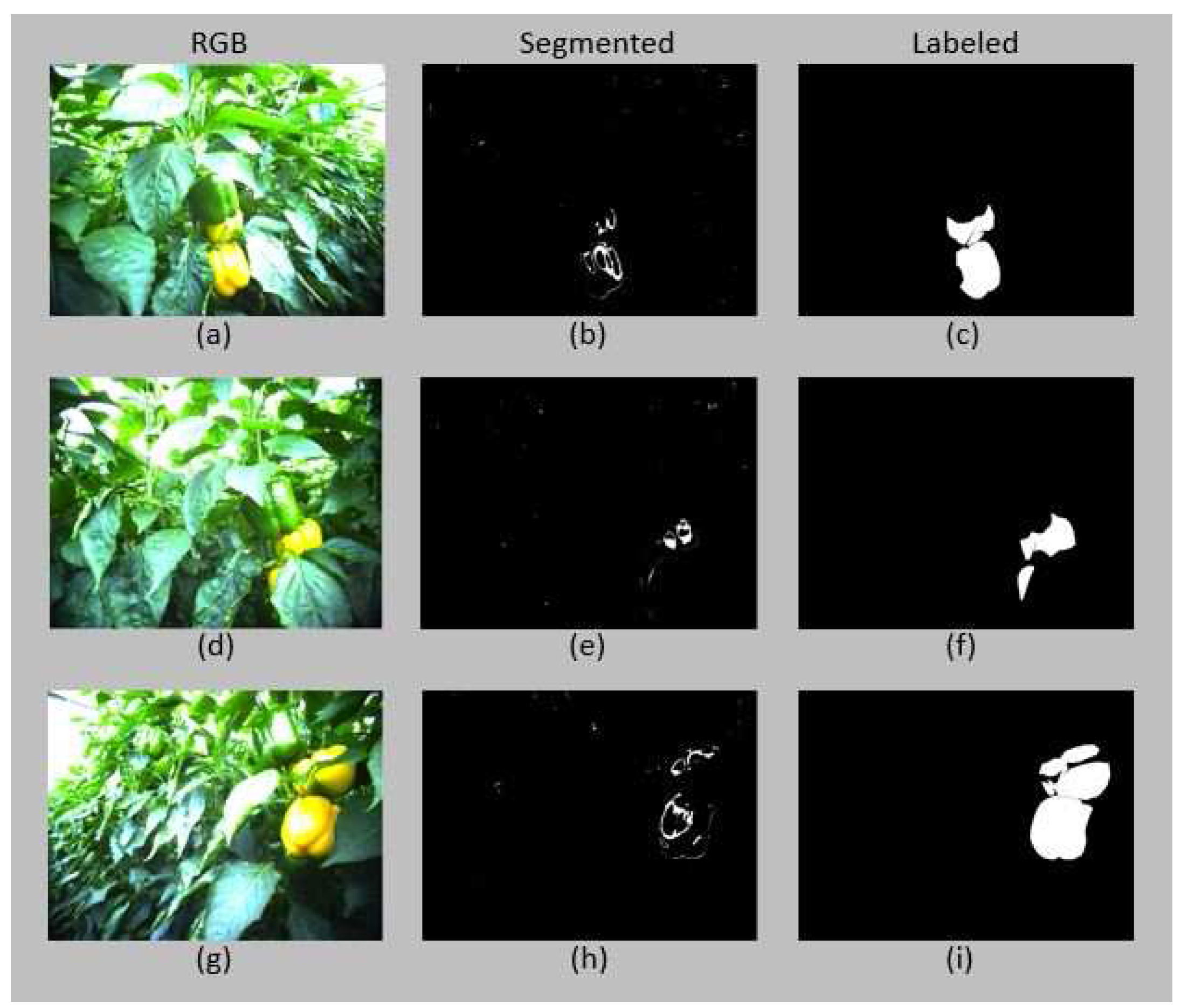
In RL the T function usually returns a new state for a given state s and action a . However, in this work the T function instead returns a new representation of the image; a segmented image. Applying the same action to different images at the same state (centroids of feature clusters) results in different segmented images as shown in Figure 6, and consequently dissimilar rewards. Therefore, in this work the T function is non-deterministic.

Figure 6.
Left (a,d,g): three different images from the database which belongs to the same state (centroid); Middle (b,e,h): segmentation result of applying threshold ( = 0.1, = 0.2, = 0.5, = 1) on the input images, resulting in segmentation quality 0.09, 0.12 and 0.15 for (b,e,h), respectively; Right (c,f,i,): manually labeled images of yellow peppers used as ground truth.
After applying the selected action, the process continues with comparing the segmented image with the labeled image, then segmentation quality (reward) is computed, and lastly the Q-table is updated. After this, a new iteration begins by taking a new image from the database.
3.2.4. R Function
The RL agent learns to select the optimal action (threshold) which maximizes the reward for the states of the environment (image features).
In this work, the reward function is defined as an objective function and returns a reward value which represents the similarity between the binarized and the labeled image as described in Section 2.1. The reward function is non-deterministic as it cannot be assumed that taking the same action for two different images in the same state results in the same reward value [35]. As an example, Figure 6 shows three different images within the same state resulting in different reward values when applying the same action.
3.3. Exploration-Exploitation Strategy
During the learning process there are mainly two strategies to select actions: exploration and exploitation. With exploration strategy, the agent takes different actions randomly and with exploitation, the agent takes the actions with the highest Q-value in the current state. An important challenge in RL is balancing the ratio of exploration and exploitation to enhance the performance of learning. The ratio has a large effect on learning time and RL algorithm performance.
Selecting an extreme number of actions based on exploration strategy may lead to not finding the maximum short-term reward since the actions with the highest reward might not be discovered. On the other hand, exploiting an undiscovered environment may also results to not finding the maximum long-term reward, as the selected actions may not be optimal.
There are many different approaches to balance the ratio of exploration-exploitation in RL, e.g., utilize counters [36], model learning [37], reward comparison [38], softmax [34], and -greedy [34,39]. Most often, -greedy method is selected since it is not required to memorize any exploration specific data and also in many applications it achieved near optimal results [40].
In this paper, we compared three different exploration-exploitation strategies including epsilon-greedy algorithm, decaying epsilon-greedy algorithm and Q-value difference measurement, which are described below.
3.3.1. Epsilon-Greedy Algorithm
Epsilon-greedy (-greedy) is a method for selecting actions which uses an extra value, epsilon. At each step, a randomly generated value is compared with epsilon. If it is smaller than epsilon, then a random actions is selected (exploration). Otherwise, the action with maximum Q-value is chosen (exploitation). Q-learning continues learning until it reaches the convergence criterion or reaches the bounded number of learning iterations. In this work the -greedy algorithm is used with = 0.2, 0.5 and 0.7.
3.3.2. Decaying Epsilon-Greedy Algorithm
Despite the fact that -greedy is broadly used for action selection and results in high performance, this method still lacks adaptation of the exploration-exploitation ratio during the learning progress. Therefore, in this work, in addition to classical epsilon-greedy method with hand tuned epsilon value, the decaying epsilon-greedy strategy was also tested for balancing the exploration-exploitation ratio.
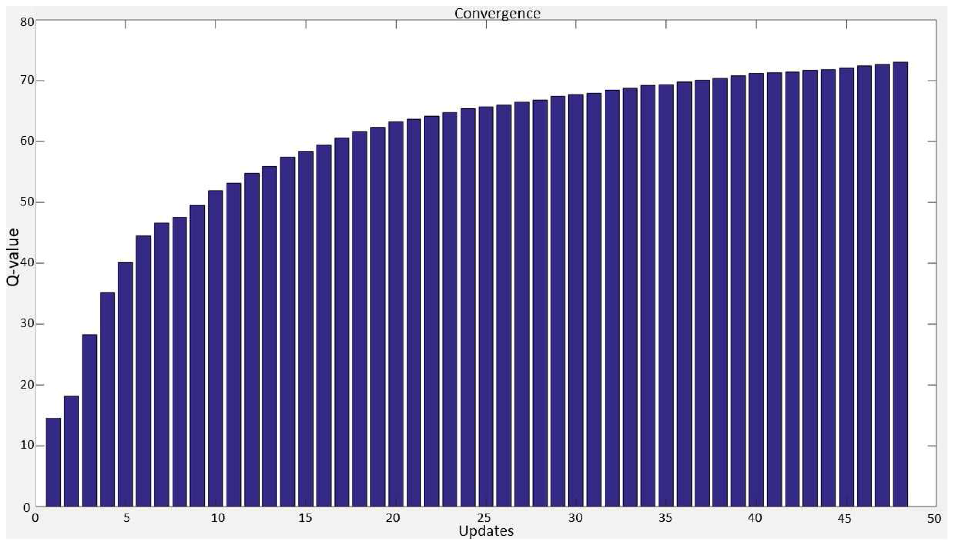
Decaying -greedy method starts with a high exploration rate and reduce it at each time step. Thus, the agent is more favored towards exploring the environment at the beginning of learning. As the agent gets more knowledge about the environment, the exploitation rate increases resulting in small or no changes in Q-values. Figure 7 shows an example of the Q-values during the learning process.
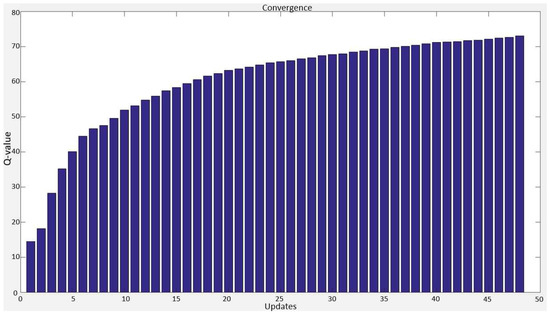
Figure 7.
Q-values during the learning process for a state-action pair using decaying -greedy strategy. Since at the beginning of the learning the number of exploration is high, changes of Q-values are large. As the process continues the exploitation rate increases, which results in more stable trend in Q-values.
3.3.3. Q-value Difference Measurement
Rather than -greedy and decaying -greedy strategies, we propose a method to switch between exploration and exploitation strategies adaptively.
Since in the beginning of a learning process the long term value of a state-action pair, , is unknown, thus we assume that the current Q-value of the selected action for the current state is the estimated value (). If the difference of current and previous Q-values is small enough, then it is near to the estimated value .
We use a measurement of Q-value difference, , as a parameter for switching between exploration and exploitation:
where i is the current iteration. We store during the progress and analyze it for the current state-action pair.
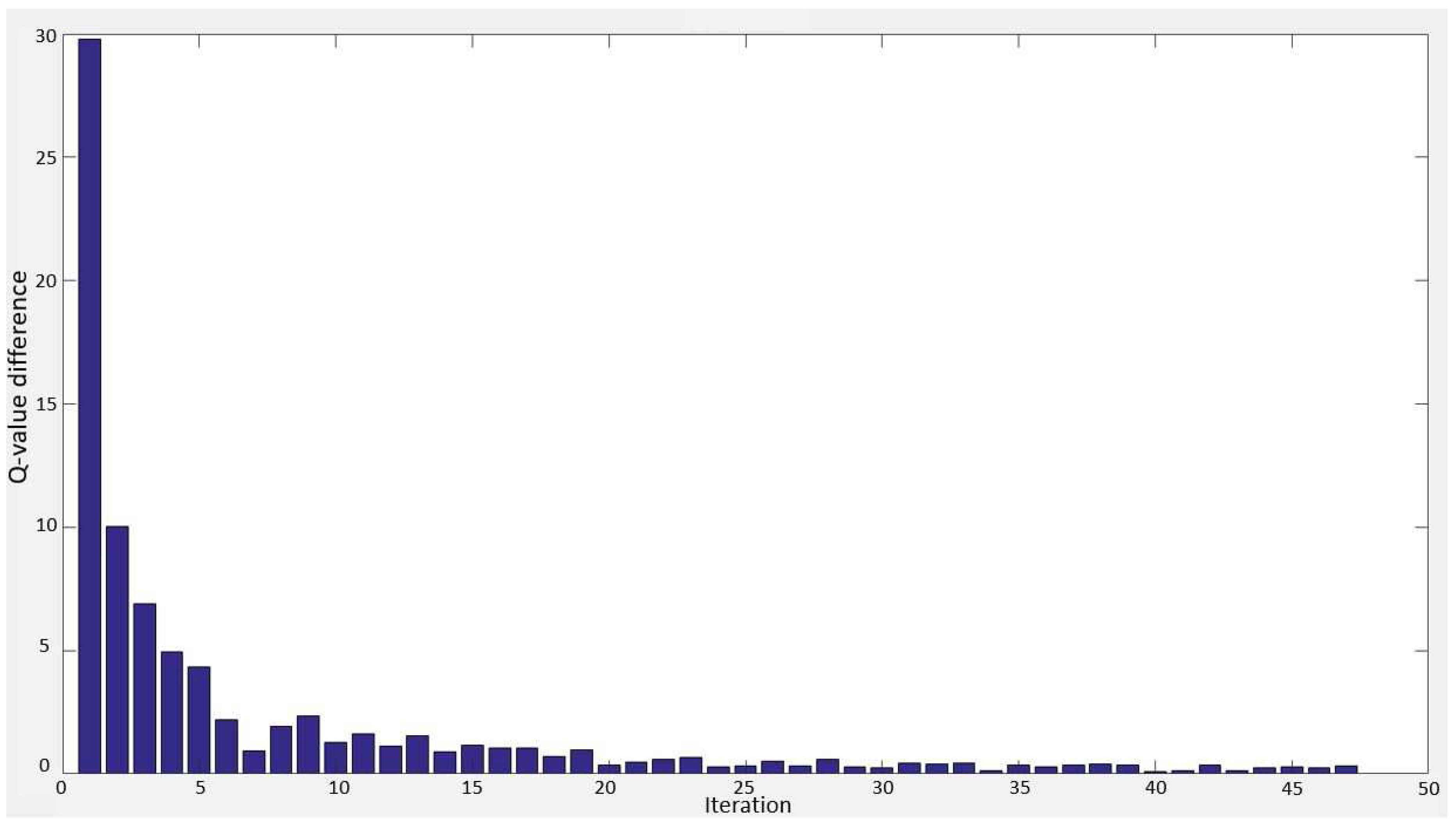
An ideal process reduces for each iteration, however, sometimes it increases. Figure 8 demonstrates an example of changes for a state-action pair in the learning process. To prevent from switching between exploration and exploitation when is small, we consider also the neighboring values by defining a sliding window with size .
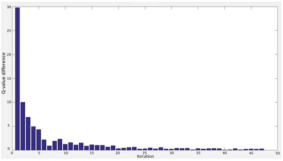
Figure 8.
Q-value differences of a state-action pair as a function iteration numbers during the learning process until it reached the convergence condition. generally decrease as the process gets closer to the convergence.
If the average of current five consecutive is larger than the average of previous five consecutive , then the strategy switches from exploration to exploitation. It means that the Q-values are not getting closer to , thus, we switch the strategy to exploitation to select the best action based on the current knowledge of the environment for the current state. Then, similar to the -greedy algorithm, the action selection strategy switches to exploration. The whole progress continues until the proposed convergence condition of the RL method is met.
3.4. Convergence
In general, RL might require tens of thousands of iterations before converging. As an example, Mitchell et al. [35] showed that the Tesauro’s TD-GAMMON needed 1.5 million of backgammon games iterations before it converged. It has been proven that the RL converges faster by reducing the learning rate during the learning process. The choice of in this work as in Equation (3), is proven by Watkins and Dayan [41] to meet the convergence conditions. In this paper we propose to stop the training when a criterion based on the expected return of the selected actions is satisfied.
One method to evaluate performance of the selected action in RL is to compute the difference between the expected return of the selected action and the optimal action [42], called expected error. This attribute has been investigated by Littlestone [43] and Kaelbling [42]. Kaelbling defined the expected error of an action a for a given state s, , as:
where is the expected return of the optimal action and is the expected return of the selected action a. The expected error, , for selecting optimal action () is 0, and for any non-optimal action .
During the learning process, the expected error of the selected actions decrease as it gets nearer to the optimal action. This means that the difference of expected errors between consecutive iterations will be reduced. We propose a convergence measurement to stop the training based on the difference of expected errors in n consecutive iterations in a state:
where i is the current iteration in state s and is a chosen threshold. Expanding and solving Equation (7), results in:
If the condition in Equation (8) is satisfied, the training is stopped. In the proposed method we use , to assure that the difference between expected error of selected actions is stable, and .
4. Training and Testing
An important characteristic distinguishing RL from other learning methods is that it uses the results of the training process for evaluation of the selected actions rather than using pre-training information about the correct action (output) [34]. This distinctive feature of RL creates the need of searching for a suitable action.
In this work a dataset with 170 labeled images of peppers in a greenhouse environment was used. The images were split into training and testing sets using 5-fold cross validation. For each image in the training phase, we first extract features to determine state of the image (see Section 3.2.1). Then, the agent using an exploration-exploitation strategy selects an action (threshold) and segments the image. The process continues by comparing the segmented image with the ground truth to compute the reward value (see Section 2.1). Afterward, the Q-table is updated using Equation (4), and the agent checks if the convergence condition is met. Images in the training set are repeatedly fed into the system until the convergence condition is met. At each time step in the training phase the action with the highest Q-value for each state can be found, called greedy action [34].
The testing phase starts when the RL method has converged. It begins with extracting features of an image to define the state in the Q-table. Then, the action with the highest Q-value for the defined state is selected as the optimal threshold. So, in testing phase we are exploiting the knowledge of the agent from action values by selecting the greedy action based on the input image.
In the next step, the segmented image using greedy action is compared with the ground truth to determine how good is the selected threshold.
5. Experimental Results
The proposed RL-based method was evaluated using different exploration-exploitation strategies as presented in Section 3.3. The performance of the proposed strategies was compared with each other, to a benchmark, to a strategy which selects actions randomly, and also with a standard optimization method. In this work, the benchmark is an exhaustive search on all actions to determine the best possible threshold for each image. Since 5-fold cross validation was used to split the data set to training and testing sets, the results are presented as an average of performance on five sets of test images. In Table 1 the average of the quality measurement (Equation (1)), q, normalized performance, , and required number of iterations for each exploration-exploitation strategy are shown. The normalized performance of a strategy is computed as:
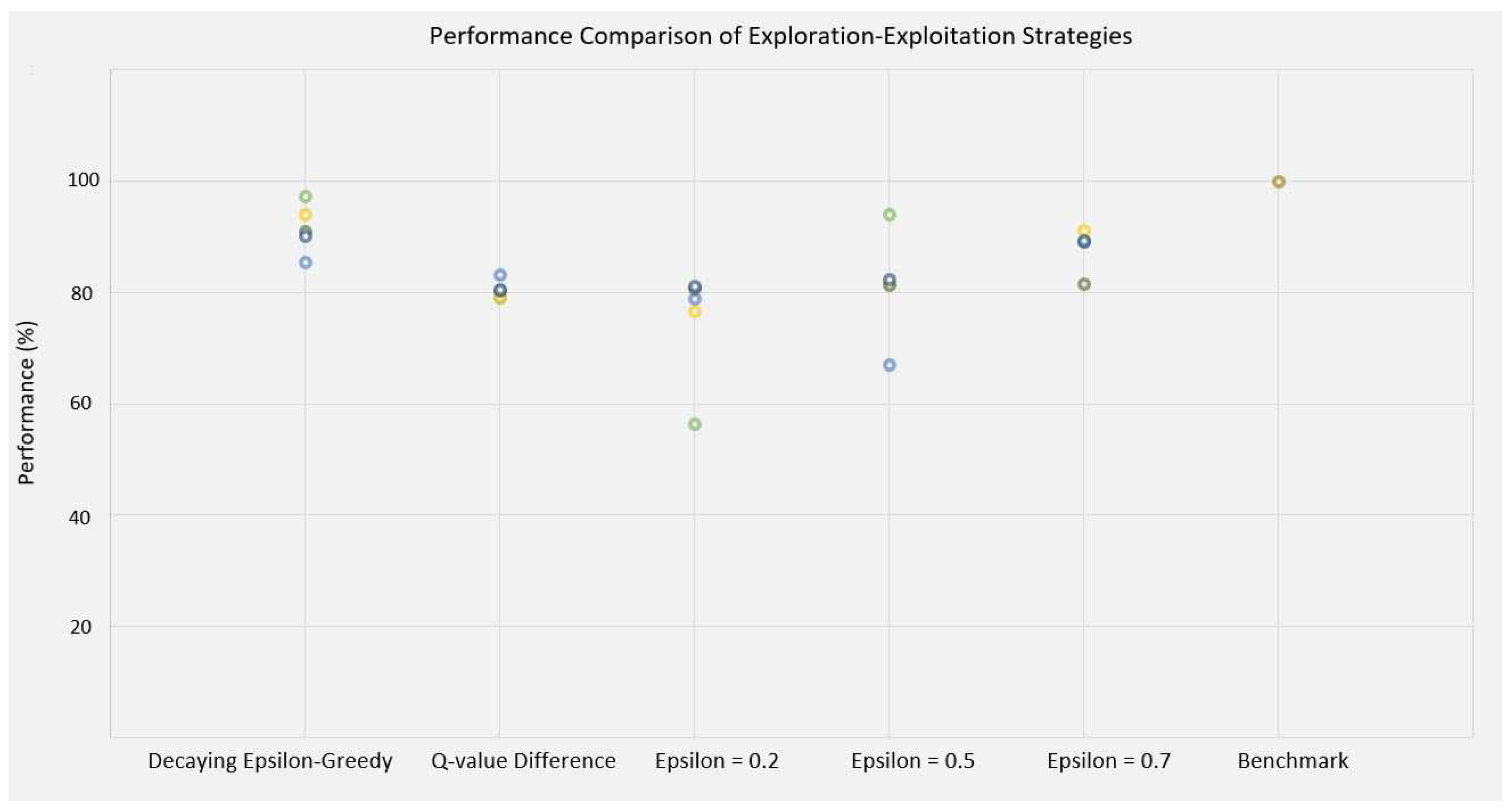
where and are the measure of segmentation quality from Equation (1) for a strategy and the benchmark respectively. Figure 9, demonstrates the normalized performance of each fold of test images for all strategies.

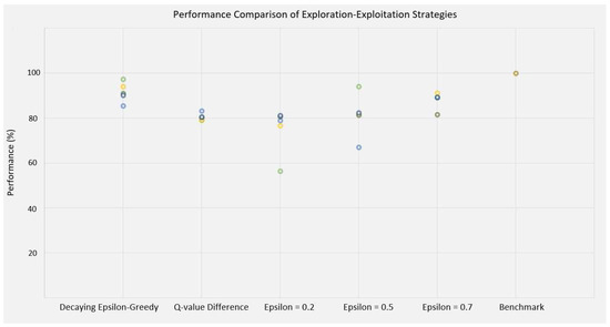
Figure 9.
Normalized performance (Equation (9)) of different exploration-exploitation strategies for each fold of cross validated test data. For comparison, the normalized performance of the benchmark (100%) is also presented. The same color of circles in different methods shows that they belong to the same fold of the test images.
In this work we consider number of iterations as the computation cost for an exploration- exploitation strategy. However, to select the best strategy we have to also consider performance of a strategy.
As depicted in Table 1, the novel exploration-exploitation strategy, Q-value difference measurement (QM), reached 80.3% of the performance achieved by the exhaustive search, with 75% less number of iterations than the benchmark. The performance increased to 87.0% using -greedy algorithm ( = 0.7), with 50% fewer required iterations compared to exhaustive search. Despite the fact that the performance increased by 6.7 percentage point (p.p), the -greedy needs twice the number of iterations for convergence in comparison to the QM algorithm.
Decaying -greedy strategy enhanced the performance to 91.5% of the benchmark, with 73% fewer iterations. This algorithm improved the performance by 11.2 p.p in comparison to the QM strategy, with similar number of iterations. It had slightly better performance than the -greedy strategy ( = 0.7) while requiring 46% fewer iterations.
Comparing the QM strategy with the -greedy algorithm with = 0.2, indicates that QM method increased the performance by 5%, however, the -greedy algorithm converged with 54% less iterations. The QM strategy and -greedy with = 0.5 had both similar performance and number of iterations. The QM strategy reached 92.0% of the performance of the best -greedy ( = 0.7) with 50.0% fewer iterations.
Considering only the computation cost, -greedy with = 0.2 converged using the least number of iteration, while also having the lowest performance of the proposed exploration-exploitation strategies. On the other hand, since decaying--greedy strategy has similar computation cost as QM and -greedy with = 0.5, lower cost in comparison to -greedy with = 0.7 and the benchmark, and also providing the highest performance among all strategies we select it as the best strategy in this work.
To check whether the RL methods is performing better than chance, we randomly selected actions for the same number of iterations as the best exploration-exploitation strategy. The results showed that randomly selected actions performed lower than any of the proposed RL methods.
Further, for the evaluation purpose, we compared the RL results with an optimization method by Jones [44]. This optimization approach is designed for finding the global minimum using Lipschitzian optimization which works without derivatives. We used a MATLAB implementation by Björkaman [45] for the tests. The optimization algorithm selected thresholds for the same number of iterations as the decaying -greedy algorithm. As it is shown in Table 1, the optimization method results to 14.1 p.p lower performance than the decaying -greedy algorithm and comes in fifth place, beating only -greedy () and random search.
With an input image of size 1600 by 1200 pixels, each iteration of the proposed algorithm took on average 85 ms with an Intel(R) Core(TM) i7 CPU, 3.40 GHz, 16 GB RAM computer. Each iteration includes, RGB to HSV conversion, extracting features and computing the centroid, selecting a threshold based on the exploration-exploitation strategies, measuring the segmentation quality, updating the Q-table and computing the convergence measurement.
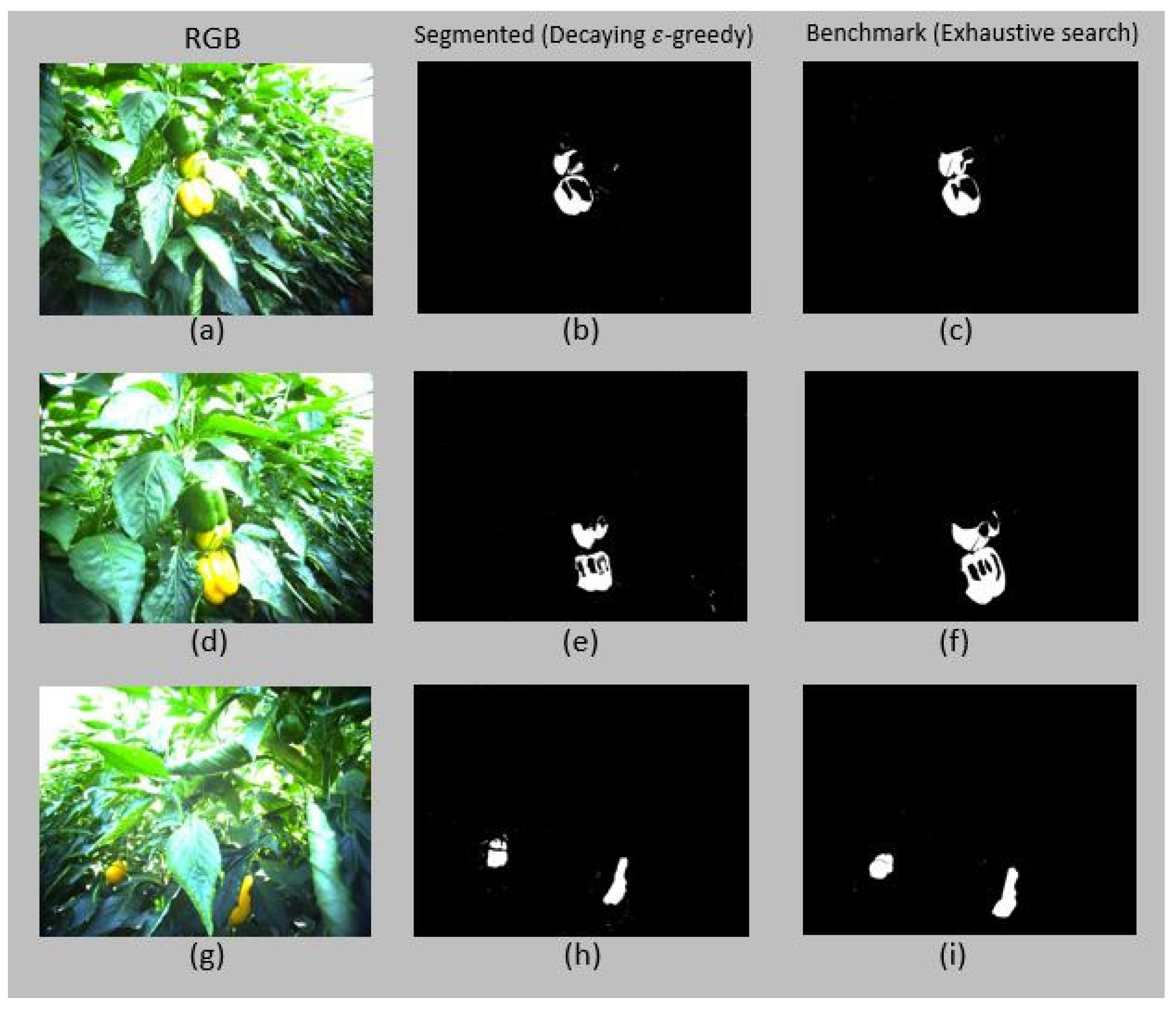
For illustration, the results of applying an optimal threshold which is selected by decaying -greedy algorithm and exhaustive search respectively to three different images which belongs to the same state (centroid) are presented in Figure 10 (see Figure 6 for the result of applying a non-optimal threshold to the same images). The optimal threshold selected by decaying -greedy algorithm was { = 0.1, = 0.2, = 0.35, = 1} with normalized performance 87%, 92% and 96% for (b), (e), and (h) respectively.

Figure 10.
The result of applying the optimal threshold selected by decaying -greedy (middle column (b,e,h)) and the benchmark (right column (c,f,i)) algorithms to three different input images (a,d,g)) which belongs to the same state (centroid). Normalized performance 87%, 92% and 96% for (b,e,h) respectively.
6. Conclusions and Future Work
Reinforcement learning is a promising method for autonomic solutions in many problems. In this work we present a reinforcement learning-based method for image thresholding. Besides the conventional exploration-exploitation strategies, a new strategy based on Q-value differences is introduced. Additionally, a convergence method based on the difference of expected errors in n consecutive iterations in a state is presented. The performance of the proposed method with different exploration-exploitation strategies are compared to the benchmark, an exhaustive search on actions (thresholds) for each image, and also to an optimization algorithm.
The highest performance was achieved by using the decaying -greedy algorithm. The results showed that the performance was 91.5% of the exhaustive search with 73% fewer iterations (computation cost). The best -greedy method ( = 0.7) decreased the performance and converged slower. The proposed Q-value difference measurement method achieved 80.3% performance of the benchmark with 7% fewer iterations than the decaying -greedy algorithm. This shows that the method needs further improvements to outperform conventional exploration-exploitation strategies.
Results of comparing the segmented images using the proposed segmentation quality method, show that it is capable of determining the difference between segmented images based on the overlap with background and foreground areas. It verifies that the proposed algorithm is an accurate method to compute the reward values in this work. Moreover, comparing results of the decaying -greedy, Q-value difference measurement and -greedy ( = 0.5) methods to the optimization algorithm demonstrated that RL methods achieved higher performance with similar number of iterations. It shows that the proposed RL algorithm is a reliable approach for adaptive image thresholding.
Convergence of Q-learning in a non-deterministic environment, like in this work, is expensive. Results demonstrated that the proposed method for convergence reduced the required number of iterations by a significant number (73% for decaying -greedy).
The system is designed to adaptively segment images of yellow peppers and results of the proposed RL method indicate that it is capable of selecting a near optimal threshold for each image from varying environmental conditions of real working scenes. The system can be trained to adaptively segment images of fruits with any color and not only yellow peppers. The fruit segmentation algorithms presented in this work can be integrated in the the sweet pepper harvesting robotic system developed in the SWEEPER project to enhance the fruit detection capabilities, especially during the visual servoing phase.
As future work, a neural network will be incorporated into the proposed method for learning the Q-values. The integrated network will be trained for each state, in which the inputs are the state actions, and the output is the set of generated Q-values for each state-action pair. In other words, the neural network will be used instead of a Q-table for storing the Q-values. It will considerably reduce the search time inside the Q-table when the size of Q-table is large. Also, Improving the performance of Q-value difference measurement algorithm using different methods of comparing the neighboring for switching between exploration and exploitation will be subject to future studies. Moreover, we will define an additional RL algorithm to determine the best set of features to be extracted from the segmented images. In this method, states would be a definition of the segmented images and actions can be described with different feature sets that would be used for classification of the segmented objects. Furthermore we intend to compare the method to existing methods for local thresholding. The efficiency of RL as search method will also be compared with stochastic gradient methods.
Acknowledgments
This research was supported by the European Commission (SWEEPER GA No. 644313). We thank our colleague Mahshid Helali Moghadam for providing expert advices on reinforcement learning.
Author Contributions
Ahmad Ostovar developed and implemented all algorithms. all authors contributed equally to the writing of this paper and evaluation of the results.
Conflicts of Interest
The authors declare no conflict of interest.
References
- Hayashi, S.; Ota, T.; Kubota, K.; Ganno, K.; Kondo, N. Robotic harvesting technology for fruit vegetables in protected horticultural production. In Proceedings of the Information and Technology for Sustainable Fruit and Vegetable Production, Montpellier, France, 12–16 September 2005; pp. 227–236. [Google Scholar]
- Hellström, T.; Ringdahl, O. A software framework for agricultural and forestry robots. Ind. Robot Int. J. 2013, 40, 20–26. [Google Scholar] [CrossRef][Green Version]
- Ringdahl, O.; Kurtser, P.; Barth, R.; Edan, Y. Operational flow of an autonomous sweetpepper harvesting robot. In Proceedings of the 5th Israeli Conference on Robotics, Hertzilya, Israel, 13–14 April 2016. [Google Scholar]
- Ringdahl, O.; Kurtser, P.; Edan, Y. Strategies for selecting best approach direction for a sweet-pepper harvesting robot. In Towards Autonomous Robotic Systems, Proceedings of the 18th Annual Conference, Guildford, UK, 19–21 July 2017; Springer: Berlin, Germany, 2017. [Google Scholar]
- Gongal, A.; Amatya, S.; Karkee, M.; Zhang, Q.; Lewis, K. Sensors and systems for fruit detection and localization: A review. Comput. Electron. Agric. 2015, 116, 8–19. [Google Scholar] [CrossRef]
- Kapach, K.; Barnea, E.; Mairon, R.; Edan, Y.; Ben-Shahar, O. Computer vision for fruit harvesting robots—State of the art and challenges ahead. Int. J. Comput. Vis. Robot. 2012, 3, 4–34. [Google Scholar] [CrossRef]
- Grift, T.; Zhang, Q.; Kondo, N.; Ting, K. A review of automation and robotics for the bioindustry. J. Biomech. Eng. 2008, 1, 37–54. [Google Scholar]
- Bac, C.W.; Henten, E.J.; Hemming, J.; Edan, Y. Harvesting Robots for High-value Crops: State-of-the-art Review and Challenges Ahead. J. Field Robot. 2014, 31, 888–911. [Google Scholar] [CrossRef]
- Bhanu, B.; Lee, S. Genetic Learning for Adaptive Image Segmentation; Springer Science and Business Media: Berlin, Germany, 2012; Volume 287. [Google Scholar]
- Haralick, R.M.; Shapiro, L.G. Image Segmentation Techniques. Comput. Vis. Graph. Image Process. 1985, 29, 100–132. [Google Scholar] [CrossRef]
- Martin, V.; Maillot, N.; Thonnat, M. A Learning Approach for Adaptive Image Segmentation. In Proceedings of the International Conference on Computer Vision Systems, New York, NY, USA, 4–7 January 2006; p. 40. [Google Scholar]
- Nalwa, V.S. A Guided Tour of Computer Vision; Addison-Wesley: Boston, MA, USA, 1994. [Google Scholar]
- Vitzrabin, E.; Edan, Y. Adaptive thresholding with fusion using a RGBD sensor for red sweet-pepper detection. Biosyst. Eng. 2016, 146, 45–56. [Google Scholar] [CrossRef]
- Vitzrabin, E.; Edan, Y. Changing task objectives for improved sweet pepper detection for robotic harvesting. IEEE Robot. Autom. Lett. 2016, 1, 578–584. [Google Scholar] [CrossRef]
- Hannan, M.; Burks, T.; Bulanon, D. A real-time machine vision algorithm for robotic citrus harvesting. In Proceedings of the 2007 ASAE Annual Meeting, Minneapolis, Minnesota, 17–20 June 2007; American Society of Agricultural and Biological Engineers: St. Joseph, MI, USA, 2007. [Google Scholar]
- Shokri, M.; Tizhoosh, H.R. A reinforcement agent for threshold fusion. Appl. Soft Comput. 2008, 8, 174–181. [Google Scholar] [CrossRef]
- Bhanu, B.; Peng, J. Adaptive integrated image segmentation and object recognition. IEEE Trans. Syst. Man Cybern. Part C (Appl. Rev.) 2000, 30, 427–441. [Google Scholar] [CrossRef]
- Peng, J.; Bhanu, B. Closed-loop object recognition using reinforcement learning. IEEE Trans. Pattern Anal. Mach. Intell. 1998, 20, 139–154. [Google Scholar] [CrossRef]
- Sahba, F.; Tizhoosh, H.R.; Salama, M.M. Application of opposition-based reinforcement learning in image segmentation. In Proceedings of the IEEE Symposium on Computational Intelligence in Image and Signal Processing (CIISP 2007), Honolulu, HI, USA, 1–5 April 2007; pp. 246–251. [Google Scholar]
- Yin, P.Y. Maximum entropy-based optimal threshold selection using deterministic reinforcement learning with controlled randomization. Signal Process. 2002, 82, 993–1006. [Google Scholar] [CrossRef]
- Bianchi, R.A.; Ramisa, A.; De Mántaras, R.L. Automatic selection of object recognition methods using reinforcement learning. In Advances in Machine Learning I; Springer: Berlin, Germany, 2010; pp. 421–439. [Google Scholar]
- Kokai, I.; Lorincz, A. Fast adapting value estimation-based hybrid architecture for searching the world-wide web. Appl. Soft Comput. 2002, 2, 11–23. [Google Scholar] [CrossRef]
- Li, H.; Venugopal, S. Using Reinforcement Learning for Controlling an Elastic Web Application Hosting Platform. In Proceedings of the 8th ACM International Conference on Autonomic Computing (ICAC 11), Karlsruhe, Germany, 14–18 June 2011; ACM: New York, NY, USA, 2011; pp. 205–208. [Google Scholar]
- Jamshidi, P.; Sharifloo, A.; Pahl, C.; Arabnejad, H.; Metzger, A.; Estrada, G. Fuzzy Self-Learning Controllers for Elasticity Management in Dynamic Cloud Architectures. In Proceedings of the 2016 12th International ACM SIGSOFT Conference on Quality of Software Architectures (QoSA), Venice, Italy, 5–8 April 2016; pp. 70–79. [Google Scholar]
- Arabnejad, H.; Jamshidi, P.; Estrada, G.; El Ioini, N.; Pahl, C. An Auto-Scaling Cloud Controller Using Fuzzy Q-Learning - Implementation in OpenStack. In Service-Oriented and Cloud Computing, Proceedings of the 5th IFIP WG 2.14 European Conference, ESOCC 2016, Vienna, Austria, 5–7 September 2016; Springer International Publishing: Cham, Switzerland, 2016; pp. 152–167. [Google Scholar]
- Wu, J.; Xu, X.; Zhang, P.; Liu, C. A novel multi-agent reinforcement learning approach for job scheduling in Grid computing. Future Gener. Comput. Syst. 2011, 27, 430–439. [Google Scholar] [CrossRef]
- Vengerov, D. A reinforcement learning approach to dynamic resource allocation. Eng. Appl. Artif. Intell. 2007, 20, 383–390. [Google Scholar] [CrossRef]
- Gonzalez, R.C.; Woods, R.E. Image processing. In Digital Image Processing, 2nd ed.; Pearson: London, UK, 2007. [Google Scholar]
- Bovik, A.C. Handbook of Image and Video Processing; Academic Press: Cambridge, MA, USA, 2010. [Google Scholar]
- Sezgin, M.; Sankur, B. Survey over image thresholding techniques and quantitative performance evaluation. J. Electron. Imaging 2004, 13, 146–168. [Google Scholar]
- Yan, H. Unified formulation of a class of image thresholding techniques. Pattern Recognit. 1996, 29, 2025–2032. [Google Scholar] [CrossRef]
- Huang, L.K.; Wang, M.J.J. Image thresholding by minimizing the measures of fuzziness. Pattern Recognit. 1995, 28, 41–51. [Google Scholar] [CrossRef]
- Fang, Y.; Yamada, K.; Ninomiya, Y.; Horn, B.K.; Masaki, I. A shape-independent method for pedestrian detection with far-infrared images. IEEE Trans. Veh. Technol. 2004, 53, 1679–1697. [Google Scholar] [CrossRef]
- Sutton, R.S.; Barto, A.G. Reinforcement Learning: An Introduction; MIT Press: Cambridge, MA, USA, 1998; Volume 1. [Google Scholar]
- Mitchell, T.M. Machine Learning; WCB: Edmonton, AB, Canada, 1997. [Google Scholar]
- Thrun, S.B. Efficient Exploration in Reinforcement Learning; Carnegie Mellon University: Pittsburgh, PA, USA, 1992. [Google Scholar]
- Brafman, R.I.; Tennenholtz, M. R-max-a general polynomial time algorithm for near-optimal reinforcement learning. J. Mach. Learn. Res. 2002, 3, 213–231. [Google Scholar]
- Ishii, S.; Yoshida, W.; Yoshimoto, J. Control of exploitation—Exploration meta-parameter in reinforcement learning. Neural Netw. 2002, 15, 665–687. [Google Scholar] [CrossRef]
- Watkins, C.J.C.H. Learning from Delayed Rewards. Ph.D. Thesis, University of Cambridge, Cambridge, UK, 1989. [Google Scholar]
- Tokic, M. Adaptive ε-greedy exploration in reinforcement learning based on value differences. In Proceedings of the 33rd annual German Conference on Advances in Artificial Intelligence, Karlsruhe, Germany, 21–24 September 2010; Springer: Berlin/Heidelberg, Germany, 2010; pp. 203–210. [Google Scholar]
- Watkins, C.J.; Dayan, P. Q-learning. Mach. Learn. 1992, 8, 279–292. [Google Scholar] [CrossRef]
- Kaelbling, L.P. Learning in Embedded Systems; MIT Press: Cambridge, MA, USA, 1993. [Google Scholar]
- Littlestone, N. Learning quickly when irrelevant attributes abound: A new linear-threshold algorithm. Mach. Learn. 1988, 2, 285–318. [Google Scholar] [CrossRef]
- Jones, D.R.; Perttunen, C.D.; Stuckman, B.E. Lipschitzian optimization without the Lipschitz constant. J. Optim. Theory Appl. 1993, 79, 157–181. [Google Scholar] [CrossRef]
- Björkman, M.; Holmström, K. Global Optimization Using the DIRECT Algorithm in Matlab. In Advanced Modeling and Optimization; Editura: Bucharest, Romania, 1999; Volume 1, pp. 17–37. [Google Scholar]
© 2018 by the authors. Licensee MDPI, Basel, Switzerland. This article is an open access article distributed under the terms and conditions of the Creative Commons Attribution (CC BY) license (http://creativecommons.org/licenses/by/4.0/).


