1. Introduction
Hexapod walking robots (HWRs) are very complex mechatronic systems where six legs are connected to a main body that performs the function of support frame. The legs are controlled with a degree of autonomy so that the robot can move within its environment, to perform intended tasks [
1]. HWRs possess clear advantages over wheeled or crawler robots noted widely in the literature such as those reported in [
2,
3,
4], since multi-legged locomotion allows obstacle climbing capability, omnidirectional motion, variable geometry, stability, access to uneven terrain, and fault tolerant locomotion. Despite the above mentioned aspects, many challenges remain before HWRs can see widespread use. Some of their current disadvantages include relatively low energy efficiency and low speed [
5]. Other key factors that have restricted a pervasive application of hexapod robots are high complexity and costs. In fact, HWRs are usually expensive machines, consisting of many actuators, sensors, transmissions, and supporting hardware [
6,
7]. The complexity of legged locomotion requires careful attention also to the control strategy by considering both path and gait planning. A discussion of these key aspects for walking hexapod robots can be found, for example, in [
8,
9,
10].
This work deals with the design of a leg-wheel walking robot named Cassino Hexapod III, which is the third version of Cassino Hexapod series. Cassino Hexapod II had a significant drawback in terms of a very complex turning strategy, since—to achieve a lightweight design—it did not have any rotational degree of freedom along vertical axis. Accordingly, the rotation of such a robot is achieved by coordinating the legs to have an oscillation of the center of mass about the middle legs, which is quite slow and inefficient. Further details on the design and control features of Cassino Hexapod II are reported in [
11,
12,
13]. Cassino Hexapod III has been fully redesigned to overcome the above issues by designing a hybrid leg, whose distal part is equipped with an omni-wheel. Additionally, Cassino Hexapod III has been completely redesigned from mechanical viewpoint to achieve a larger step size and a significantly higher payload capability as compared with Cassino Hexapod III. The proposed design solution avoids increasing the number of actuators, keeps the leg weight low, while increasing maneuverability over flat surfaces is greatly with omnidirectional motion features. It is important to point out that Cassino Hexapod III can achieve the advantages of both wheeled locomotion and legged locomotion thanks to its multi-legged hybrid design. Namely, it can be energy efficient while moving over flat surfaces by using only wheels and it can overcome obstacles as well as avoid, or at least minimize, the eventual damage to the walking surface by using its multiple legs in combination with a careful strategy in footholds positioning. This also allows useful stability features as well as fault tolerance, since the robot can still achieve its motion while one actuator or even one leg is not operational.
The paper is organized as follows:
Section 2 describes the attached problem also by referring to the milestones in HWR evolution. The proposed design procedure is described in
Section 3. A design concept of a hybrid leg-wheel HWR is presented in order to show the effectiveness and feasibility of the proposed procedure. Finally, path planning is described for the legs of Cassino Hexapod III together with its preliminary validation.
2. The Attached Problem
A great deal of literature can be found on HWRs. The evolution of HWR design was outlined for example in [
14]; an overview of the state of art of hexapod robot was also given in [
15,
16]. Some early design solutions have been for example, OSU Hexapod [
17], Odex I [
18], Aquarobot [
19], ASV [
20], Ambler [
21]. Remarkable hexapod robots in recent design solutions have included Hamlet [
22], Rhex [
23], Athlete [
24], and Lauron [
25].
In the available literature on HWRs, one can identify a very large number of solutions having many different designs and applications. Despite the high number of proposed solutions, no authors have explicitly suggested the use of HWR for applications in the domain of cultural heritage. Most of the proposed works, in fact, have focused their approach on wheeled solutions, which have well-known drawbacks in terms of mobility. This paper deals with a novel challenge in the analysis and safeguard of cultural heritage goods through the use of HWR for performing complex survey and maintenance tasks. In particular,
Figure 1a shows a specific application in Cassino: the Roman amphitheater of Cassino which dates back to the first century BC. It is one of the most typical achievements of Roman architecture that was born for typical shows of ancient Rome: the gladiatorial games. In particular, the area of interest is the paved surface that was discovered in the 1950s, (
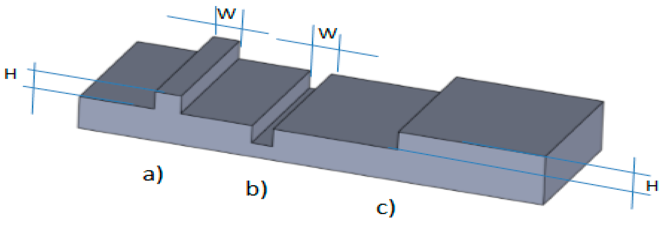
Figure 1b). The roadway is large (about 2.50 m) and has a flagstone paving stones in white limestone perfectly preserved. By referring to this operating scenario, the first robot characteristic is its capacity to move within the area under examination, carrying image capturing equipment to perform survey analyses. For this specific application, the main attention needs to be focused on walking gaits and basic operations such as step climbing, and crest and ditch overcoming. At the same time, since the surface is delicate and extremely irregular, in addition to motion the robot must also ensure that the image capturing equipment remains always horizontal so that the image post processing and reconstruction can always refer to the same horizontal plane. Since the variety of irregular terrain is very large, it is difficult to cover all the different cases of operation. In order to study this problem systematically, the real features have been simplified into standard geometric features.
Figure 2 shows the geometric features and related parameters that have been considered in term of crests, ditches, and vertical steps. Typical values have been identified as reported in
Table 1, by referring to previous experiences at the LARM Laboratory.
3. The Proposed Design Procedure
The proposed design procedure has been divided in two main stages as proposed in [
26]. The first stage consists of a preliminary architecture design. The second stage is focused on the necessary design refinements. A preliminary design is usually a trade-off solution between design requirements and key features. A systematic preliminary design procedure for HWR has been developed as referring to specific functional requirements and relationships between the design configuration and the robot capabilities or key features for specific tasks such as reported in [
26,
27,
28,
29,
30,
31,
32,
33,
34].
This section aims to design a HWR for tasks such as the inspection and operation in archeological sites, as reported for example in [
27]. Based on this selected application, key feature requirements can be summarized as follows:
- -
low-cost both in design and operation (<1000 Euros);
- -
user-friendly operation, also for non-expert users;
- -
wireless operation;
- -
capability to negotiate obstacles:
- -
a crest, with maximum width W = 100, height H = 60 mm;
- -
a ditch, with maximum width W = 100 mm;
- -
a step, with maximum height H = 60 mm;
- -
capability to carry surveying devices;
- -
operating speed on regular terrain >0.1 m/s;
- -
operating speed on uneven terrain >0.05 m/s;
- -
payload >1 kg;
- -
continuous operation in walking mode >1 h;
- -
continuous operation in omni-wheels mode >3 h.
Several sensors can be considered for identification of environment and obstacles such as Lidar, 3D scanning, sonar, radar.
Design refinements have been carried out by considering the outcome of the preliminary design step. Then, several models and analyses have been carried out for achieving a suitable refined design. For example, it has been considered the kinematic and dynamic model of one leg, and the dynamic model of one leg and of the whole body in order to identify proper components (motors, sensors, control hardware) and proper robot sizes.
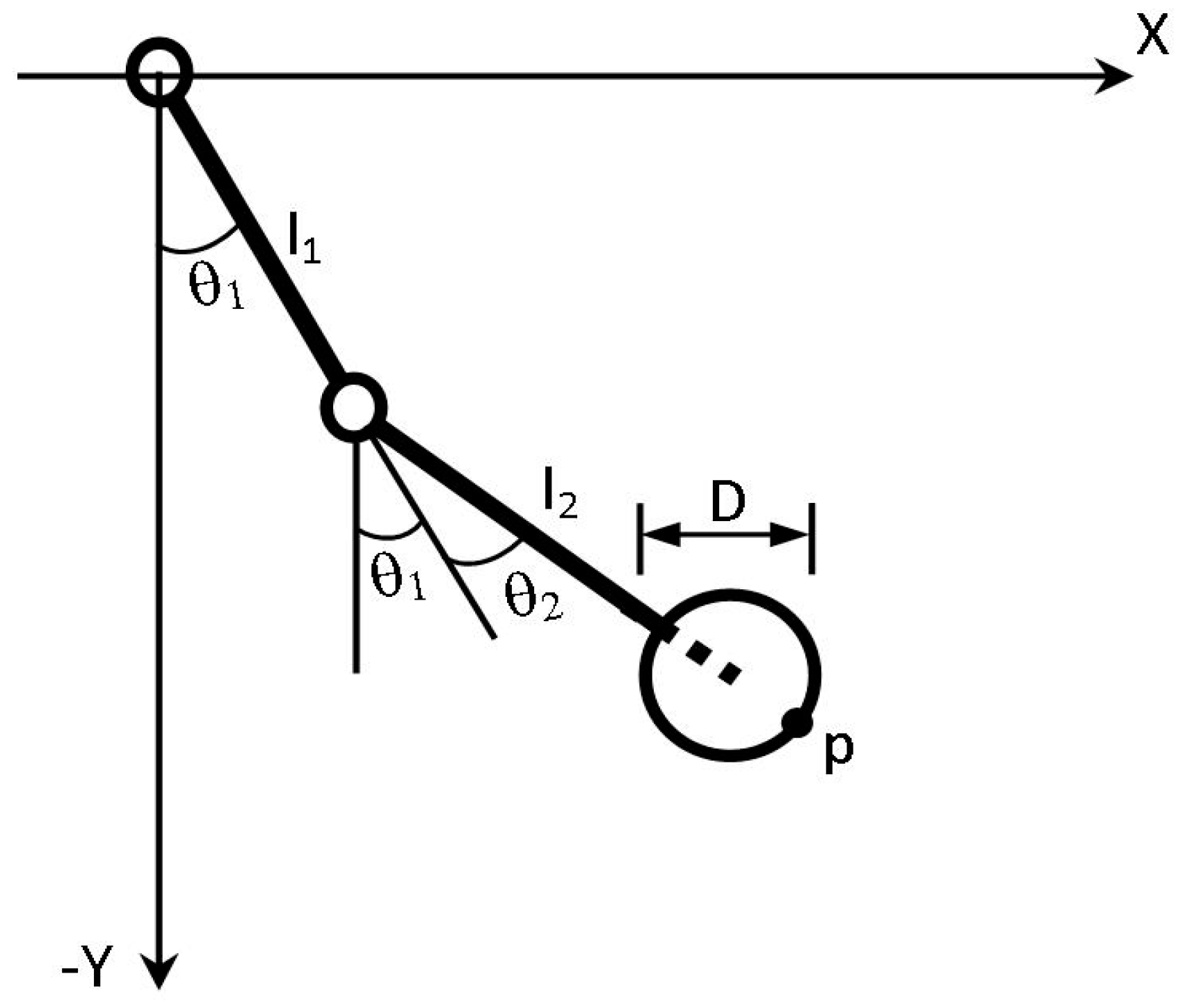
3.1. Kinematic Model of One Leg
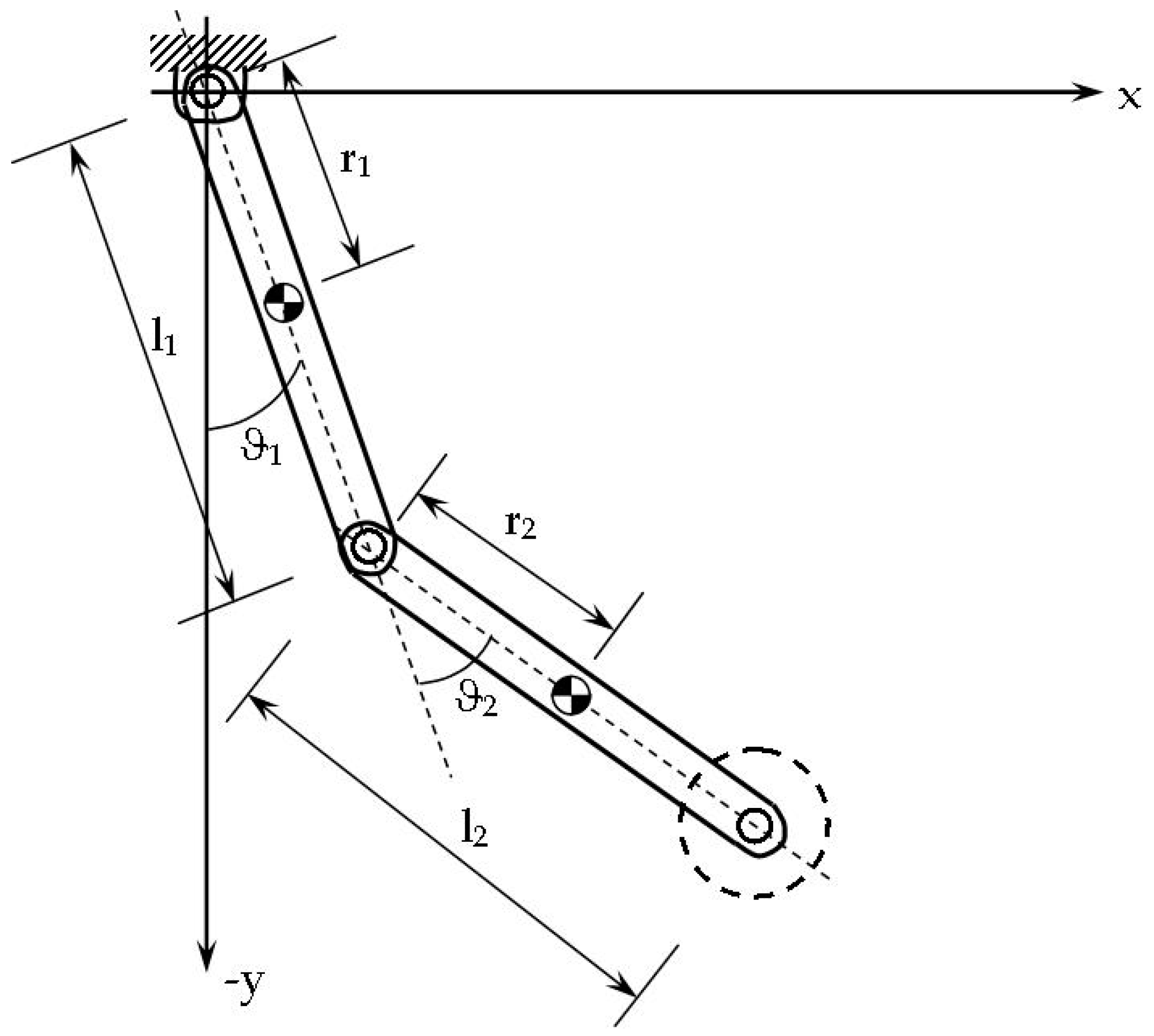
Figure 3 shows a kinematic model of the proposed leg architecture. Leg kinematics consist of two links that are connected through a knee joint. Each of the legs has three DOFs: two of them have a movement that has a range between −90 and 90 deg. that allow the robot to overpass obstacles and to walk without moving the wheels. The third motor allows to move the wheels in a full rotation range. Forwards kinematics is described by Equation (1).
Inverse kinematics can be solved calculating
where
similarly
where
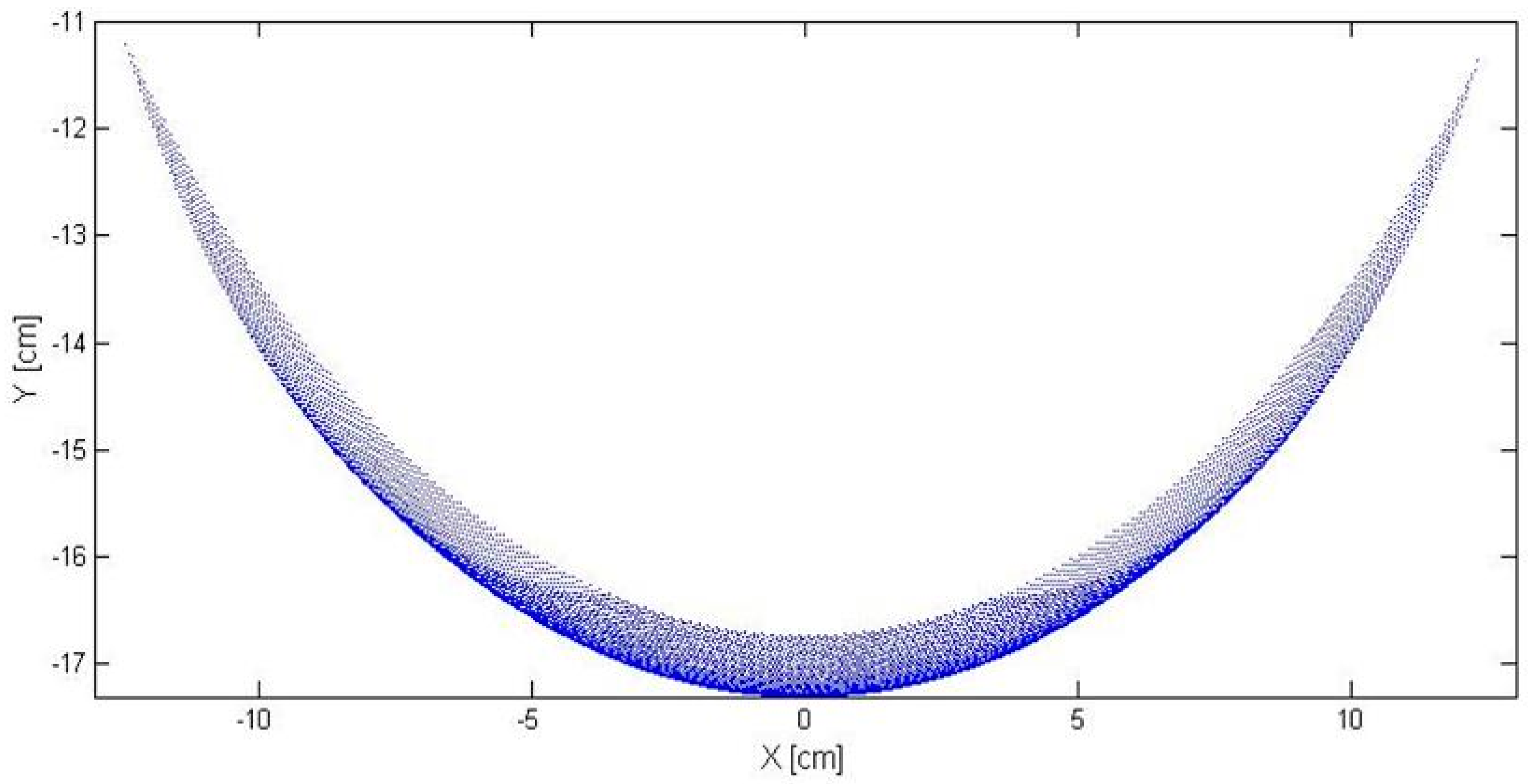
Figure 4 reports as example, a MATLAB plot of reachable area by single leg. The work area has been defined by referring the end-point p, by considering 0° <
θ1 < 30°, −30°
< θ2 < 0°,
l1 =
l2 = 70 mm D = 66 mm.
The proposed kinematic architecture can be seen as a tradeoff solution to limit the number of required actuators while achieving a sufficient mobility of the leg.
3.2. Dynamic Model of One Leg—Transfer Phase
The selection of proper actuators has required an estimation of needed motor torque. For this purpose, a preliminary dynamic model of robot leg has been carried out by means of a Lagrange formulation. This model can perform a preliminary actuator choice and leg size synthesis.
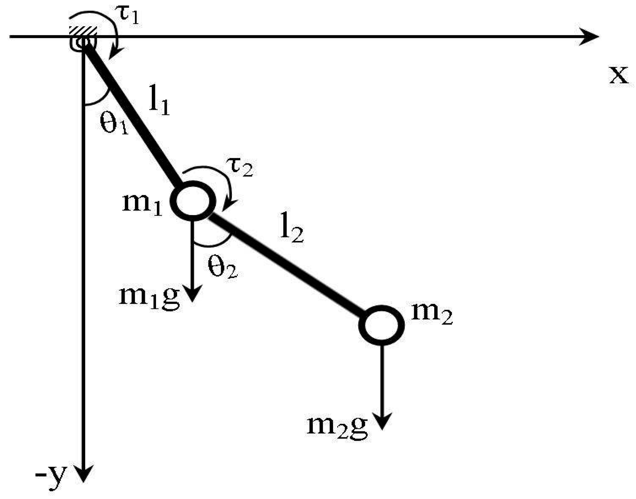
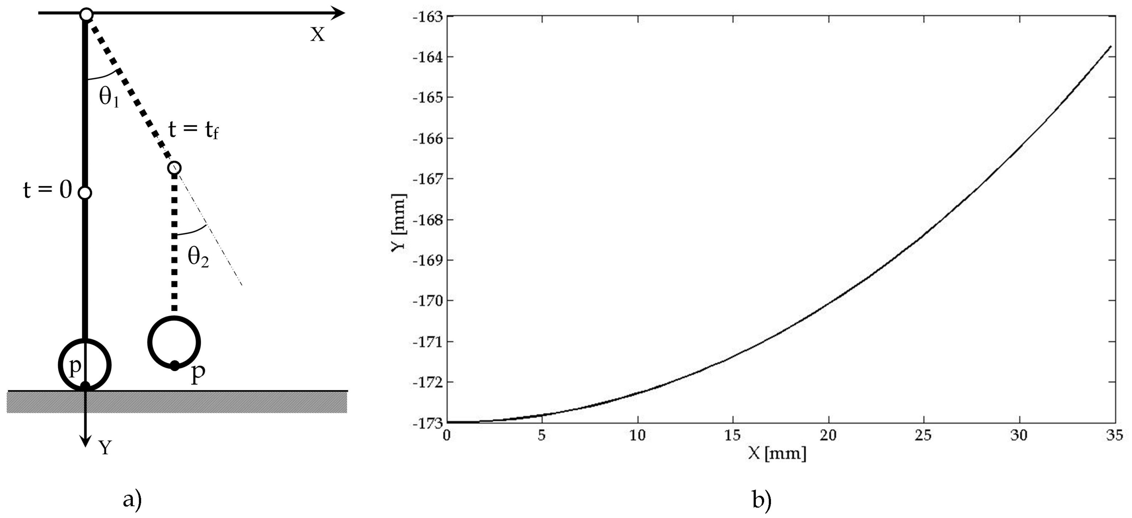
Figure 5 shows a scheme of the proposed preliminary dynamic model. It is composed of two revolute joints and two links. The masses are considered to be lumped at the edge of each link, inertia is considered negligible at this stage by referring to slow static walking.
The dynamic model of a two-joint robot leg can be written in the Lagrangian form as
where
θ is the joint variable vector and
τ is the vector of generalized forces acting on the robot manipulator.
M(
θ) is the inertia matrix,
are the Coriolis/centripetal forces, and
G(
θ) is the gravity vector. In Equation (8) we are not taking into account the friction torques since we consider them as negligible. The dynamic model of the two-link planar arm can be written by substituting the following data in Equation (8)
where
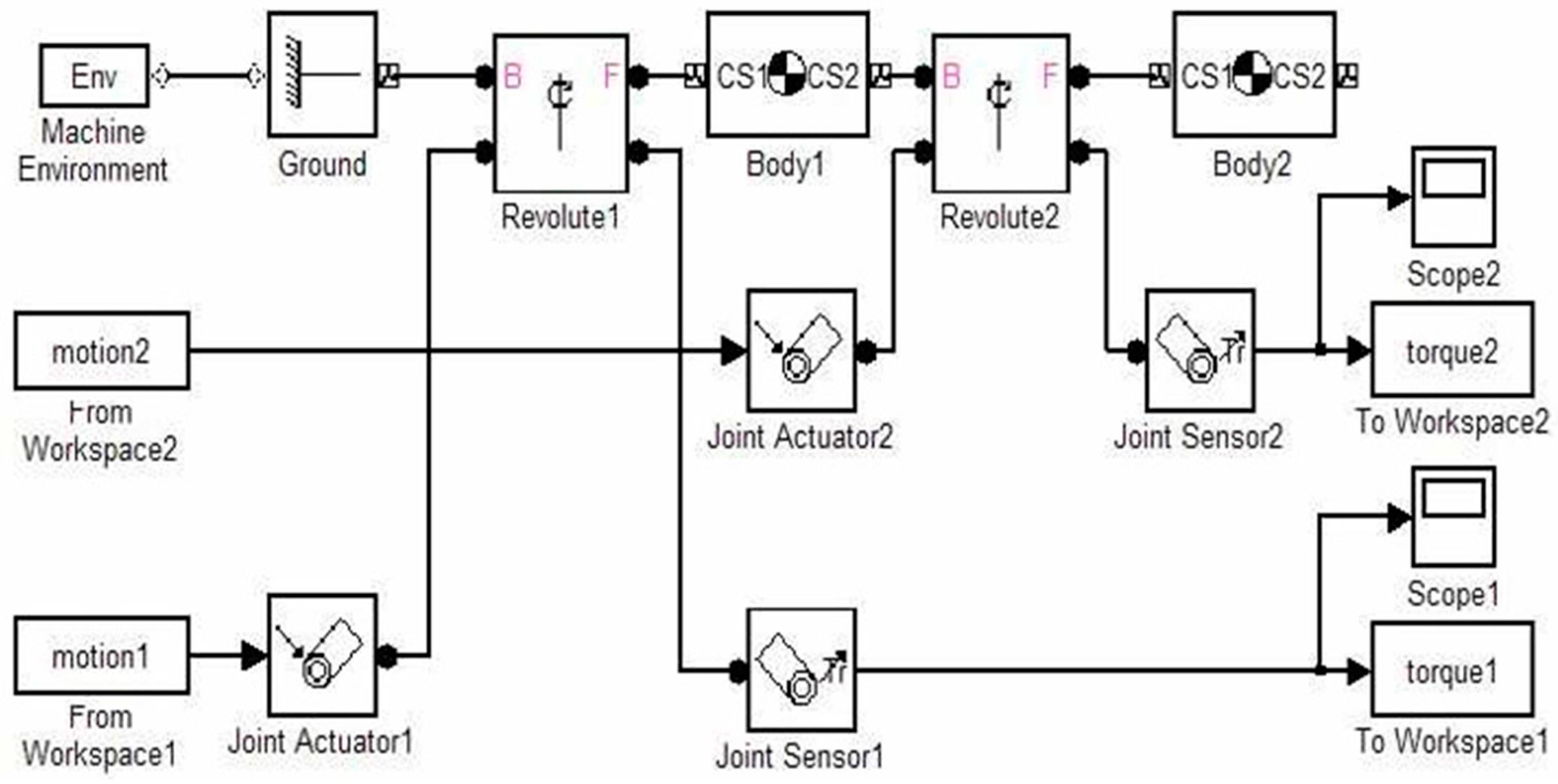
The dynamic model for transfer phase was also implemented in SimMechanics environment, as aid for the leg sizes synthesis process and also in order to estimate the needed actuator torques.
Figure 6 shows the SimMechanics model that can find the torques
τ1 and
τ2 required to obtain a prescribed movement of robotics leg as referring to the model and formalism in the scheme of
Figure 6, further details on simulation symbolism and operation can be found, for example, in [
32].
Figure 7 shows an example of trajectory that has been tested. The end-point p is moved from the initial to the goal position, along a trajectory with a predefined path.
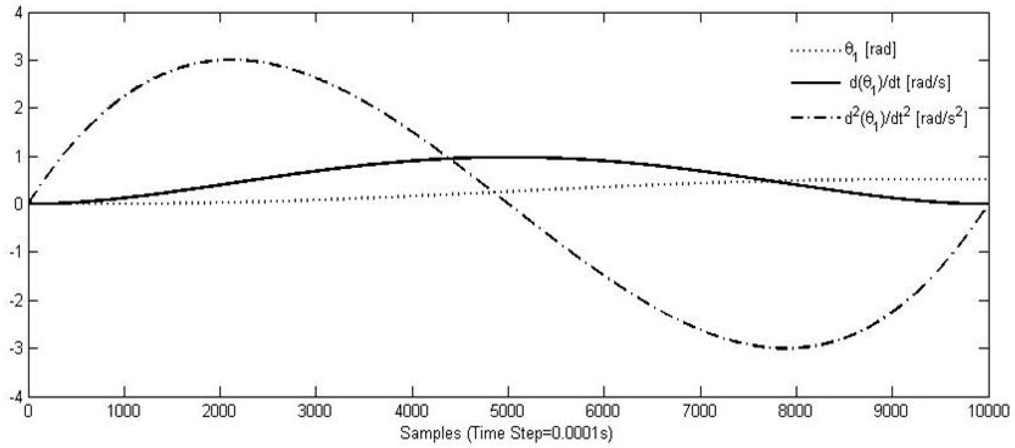
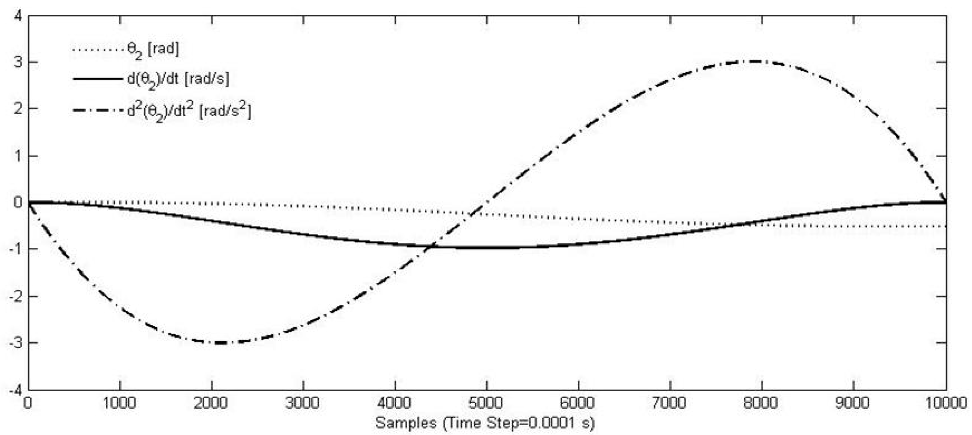
Figure 8 and
Figure 9 show, for example, the workspace variables in terms of angular displacements, velocities, and accelerations that have been considered as joint inputs for the simulation. A fifth degree polynomial has been chosen for the angular rotations interpolation. At the beginning as well as at the end point of the movement, the velocity and acceleration of point p has been set equal to zero.
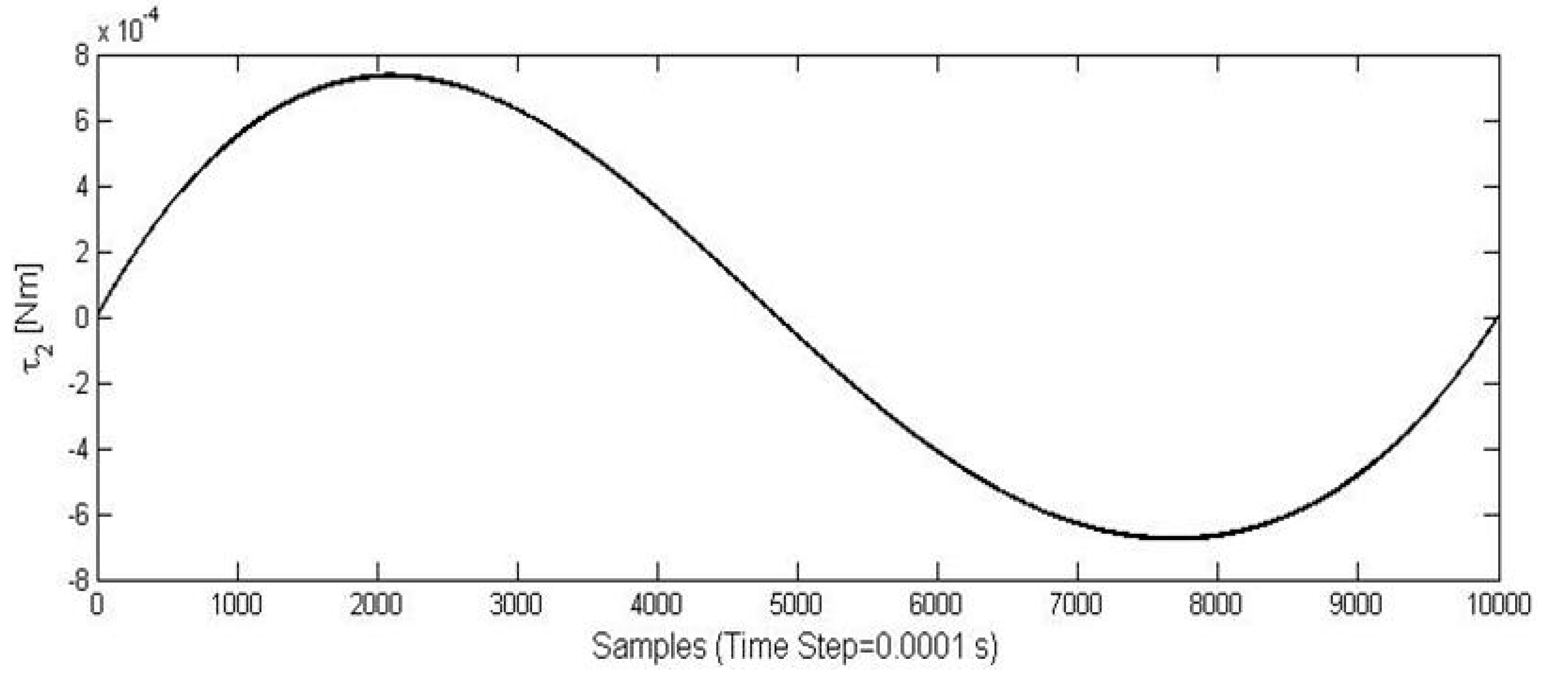
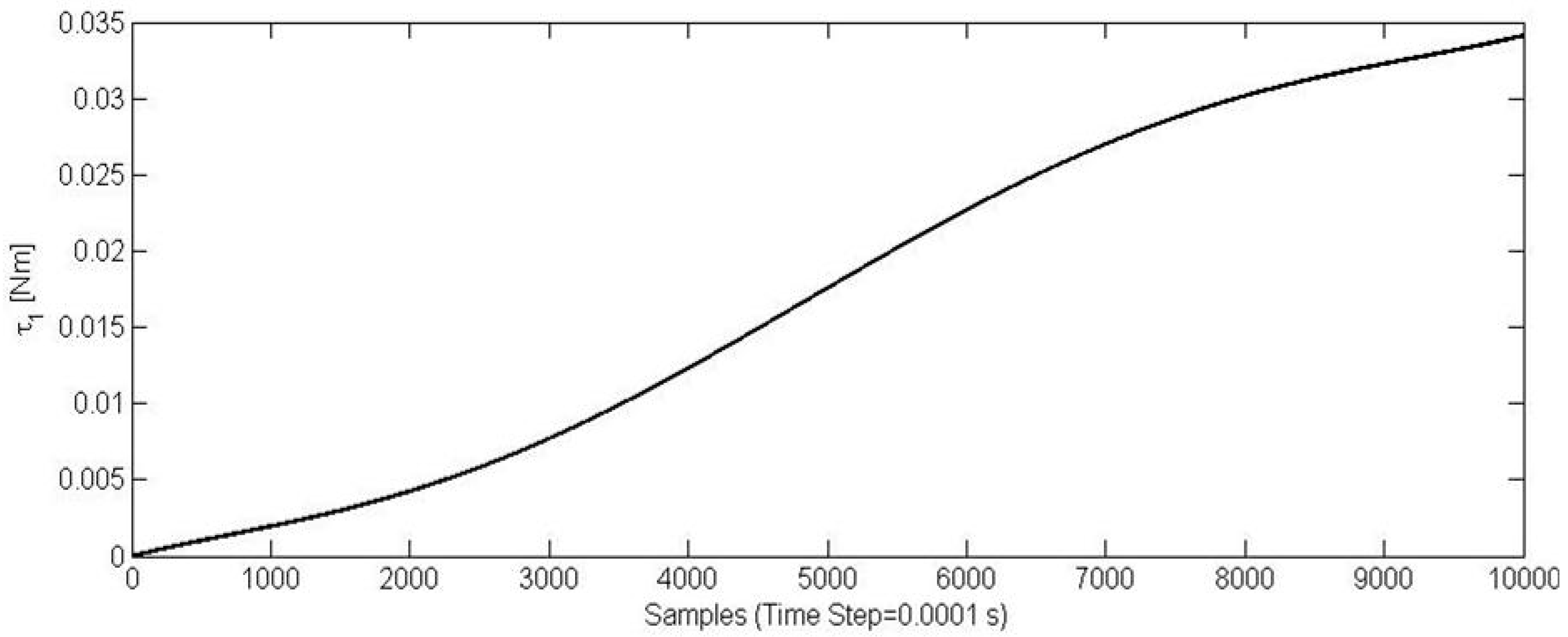
Figure 10 and
Figure 11 show time diagrams of torques
τ1 and
τ2 that have been obtained by solving the proposed model in Equations (8)–(16) for the specific trajectory that is shown in
Figure 9.
3.3. Actuator Type
The adopted actuator can be a digital servo model DS RDS3115MG [
35] since they are small, light, and low-cost. Max torque is 1.47 Nm at 6 V. Weight is 0.06 kg. Continuous rotation servo for wheels operation can be the RC servo model DS AS3103PG [
35]. Max torque is 0.39 Nm at 6 V. Weight is 0.04 kg. The feasibility of the proposed solution will be validated by means of a dynamic simulation of the whole robotic system.
3.4. Dynamic Model of the Hexapod
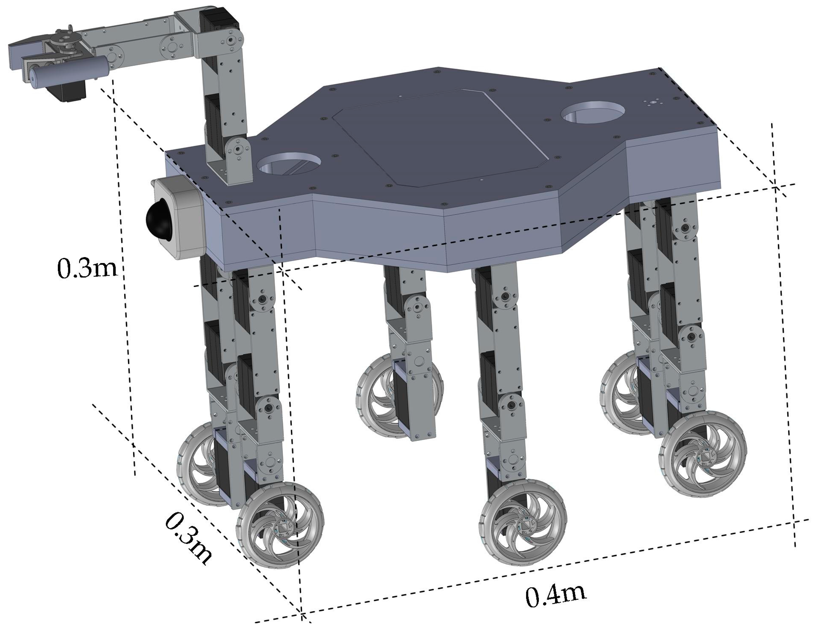
The low-cost design of the leg architecture has been obtained by using a mechanical solution with few components made with aluminum and by selecting as much as possible commercial components. The proposed leg measures 160 mm in length, 45 mm in width, and 20 mm in depth. The total weight is about 2.5 N. It has been chosen to use Mecanum-wheels with a 60 mm diameter. Mecanum-wheels are wheels with small discs around the circumference which are inclined 45 degrees to the rolling direction. The effect is that the wheel can roll, but can also slide laterally. The proposed solution has been adopted in order to allow the changing of direction strategy in wheeled operation. SolidWorks environment has been used for carrying out simulations of the proposed design solution due to its convenient features in structure analysis and in the operation study of multi-body systems. Simulations have been carried out investigating basic robot performances in a virtual environment in order to check the design feasibility before prototyping. The overall robot configuration is presented in
Figure 12. The hexapod can fit into a cube of 0.4 × 0.3 × 0.2 m. Total weight of the robot is about 30 N.
The Lagrange formulation can also be used to define a dynamic model of the overall robotic system, as proposed in [
36,
37]. The total kinetic energy is given by the sum of the kinetic energy of the main body
TB, legs
Tli and wheels
Twi
where
by referring to
Figure 13 the kinetic energy of a single leg is
The total potential energy of the robot is represented by the sum of the potential energy of the body and of the six legs
where
The potential energy of a single leg is
The Lagrange formulation can be written as
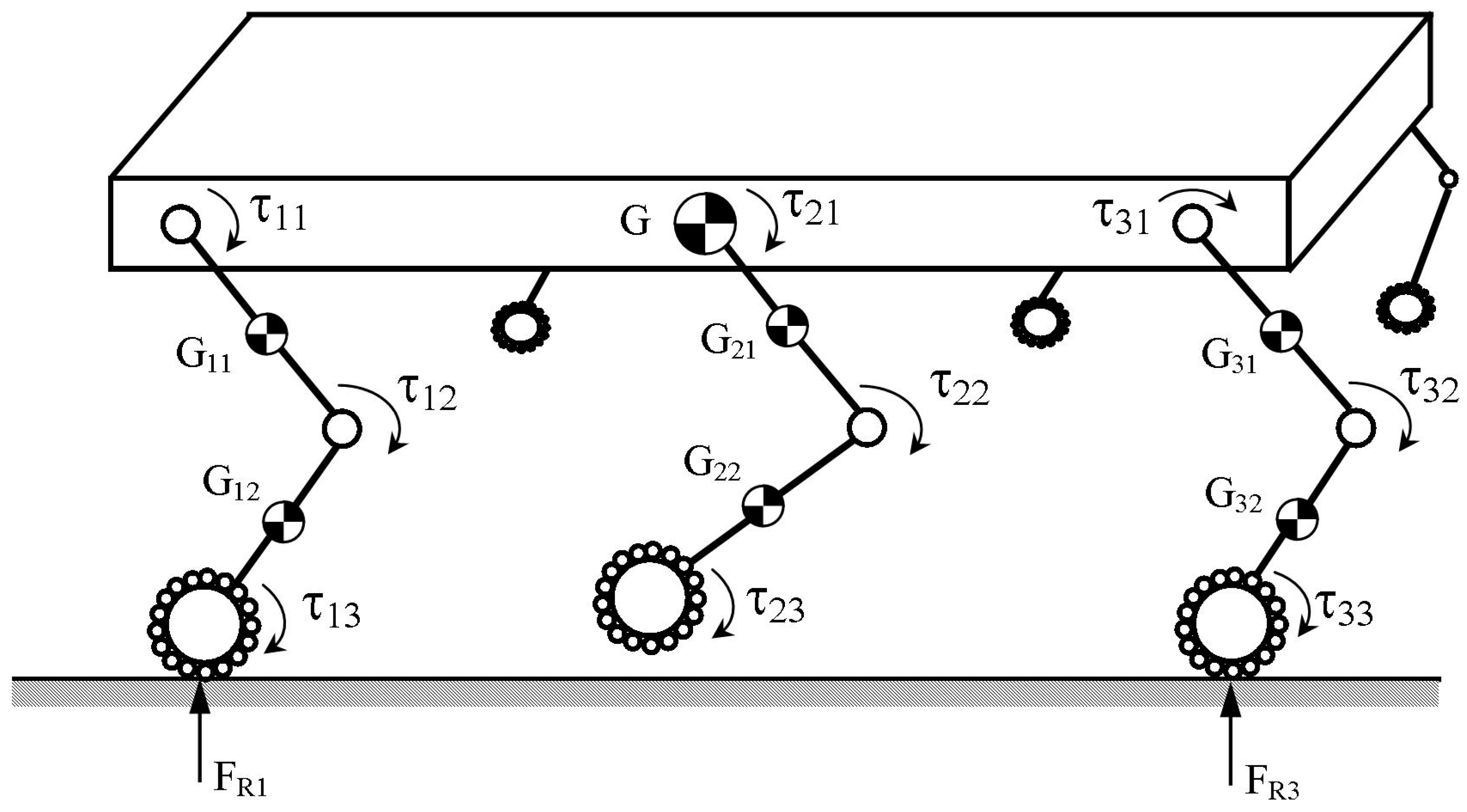
The dynamic behavior of a hexapod robot has been also modelled according to
Figure 14. Dynamic simulation of the whole hexapod has also been carried out in MSC.ADAMS environments such as outlined in [
30]. In particular, the model can take in to account several aspects—such as external forces, gravity, contacts constraints, friction, and inertia properties. The model has been elaborated by introducing each component with its specific characteristics in terms of material, mass, density, shape, and mechanical design as referring to the proposed solution. Servomotors have been modelled by using the results that have been obtained in the simulation of one leg transfer phase. Simulation shows that actuators and leg architecture can be suitable for operating the hexapod.
3.5. Control Architecture
A low-cost control architecture has been developed by using a commercial control card Arduino Mega 2560, by referring to previous experience at LARM in Cassino [
33,
34,
35]. The remote interface has been achieved by means of an Arduino Wi-Fi shield such as outlined in [
35]. The high level remote control was developed in a Java environment. The proposed solution allows task planning between a Wi-Fi network using a PC or smartphone interface. A Li-Po battery 7.4 V-2600 mAh, has been selected as suitable power supply. The overall weight of the battery is 0.35 kg.
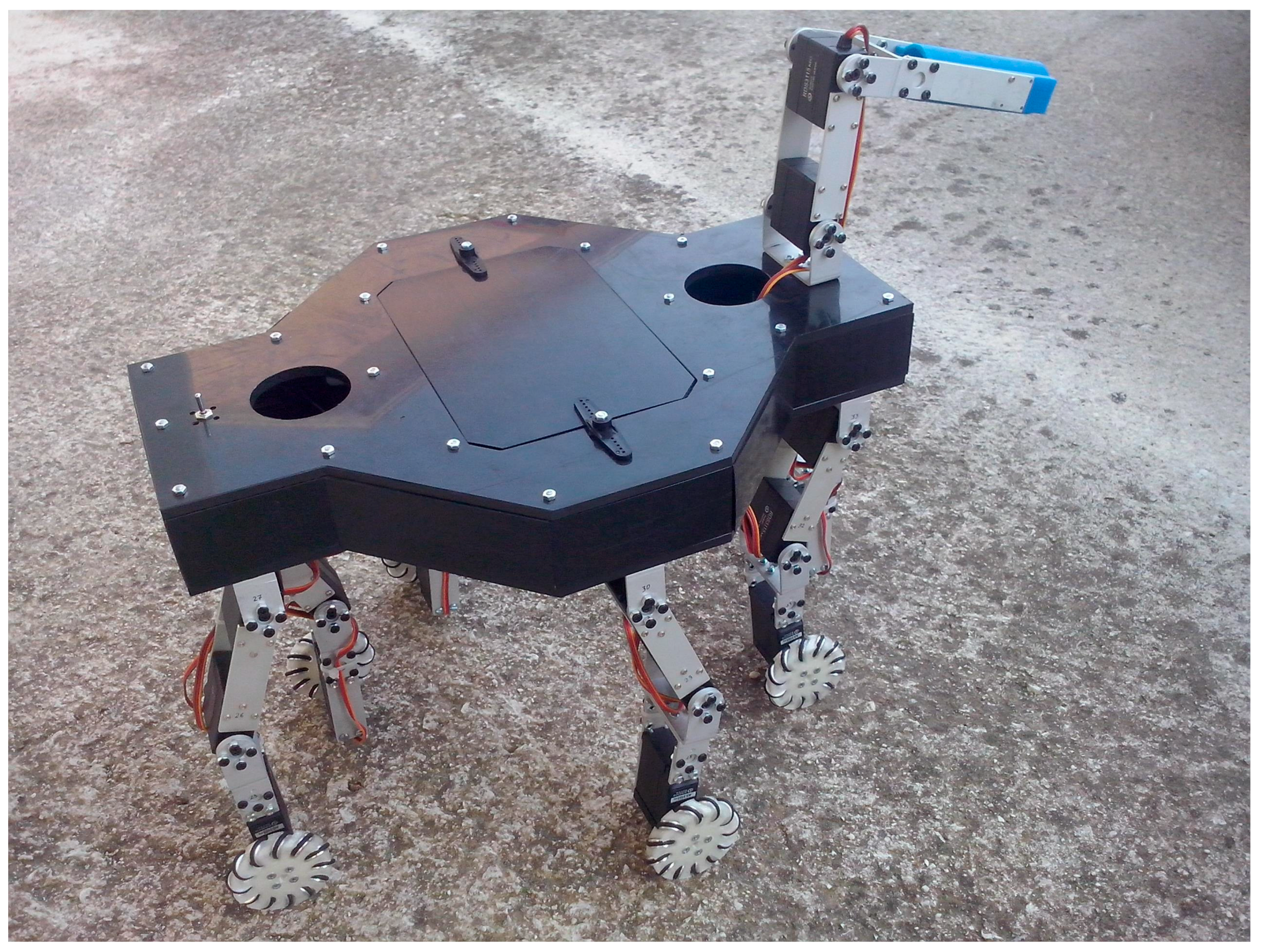
Figure 15 shown a prototype of Cassino Hexapod III that has been developed at LARM. Component manufacturing has been carried out by using a CNC milling machine. The degree of autonomy of the path planning layer includes active human robot interaction. The high level remote control can be made by using a PC or a smart device that will send a task planning to the robot by using the Wi-Fi network. At this stage, obstacles or ditches are detected by means of the camera visual feedback.
4. Leg Path Planning
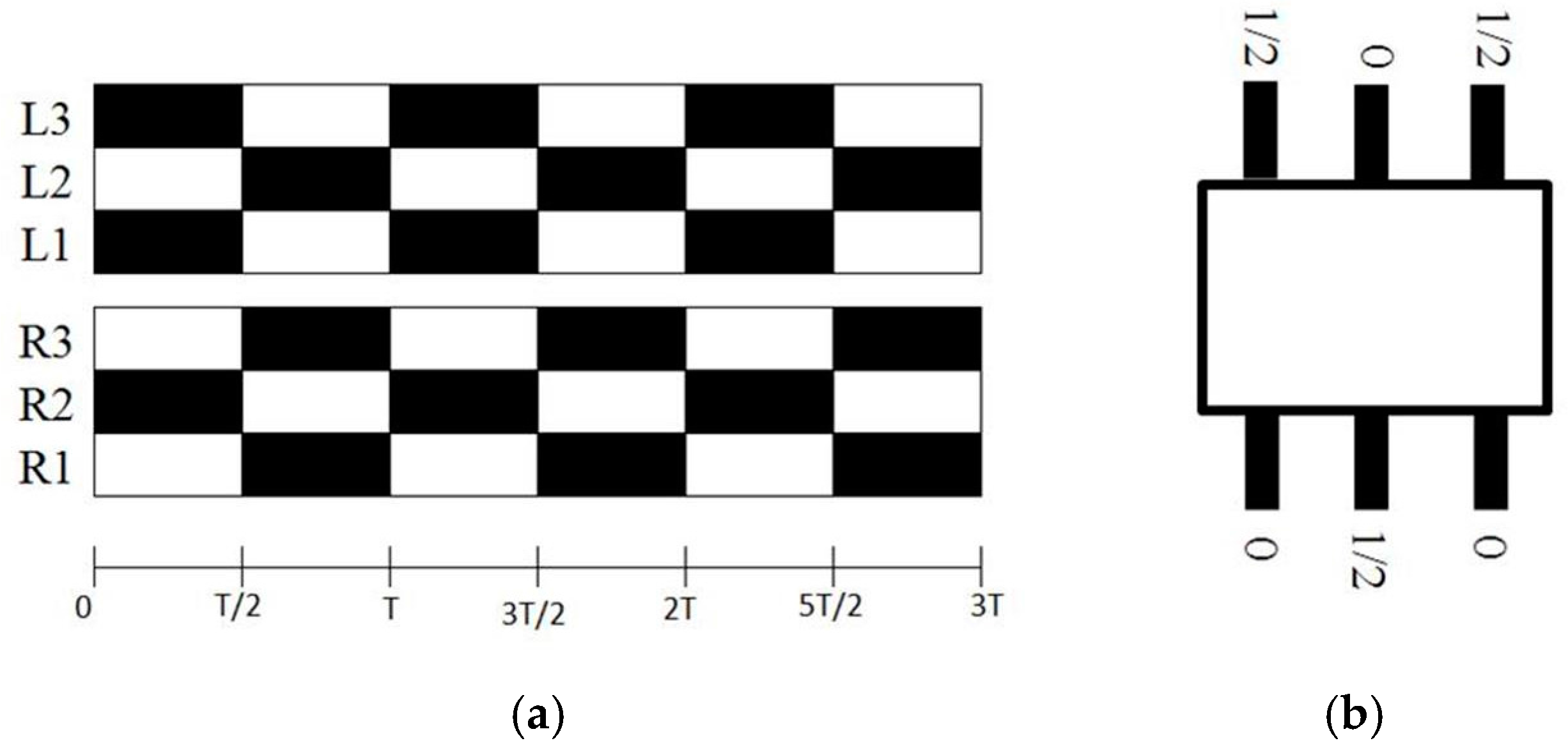
It is worth noting that the study of the gait and kinematic analysis is specifically needed only when obstacles exceed the radius of the wheel so that the wheel alone is unable to overcome them. In principle, a longer leg will be able to overcome higher obstacles provided that the leg has the same kinematic architecture and the same modular design (each module having identical size). Otherwise, search algorithms and optimal design procedures can be used to optimize the leg size in comparison with an obstacle size. The legs path planning has been defined by referring to a tripod gait strategy. Tripod gait consists in front and back legs on one side lifting simultaneously with the contralateral middle leg, forming alternating tripods as shown in
Figure 16a.
Figure 16b shows the legs phase relations: each of contralateral leg pairs has a phase shift of half period.
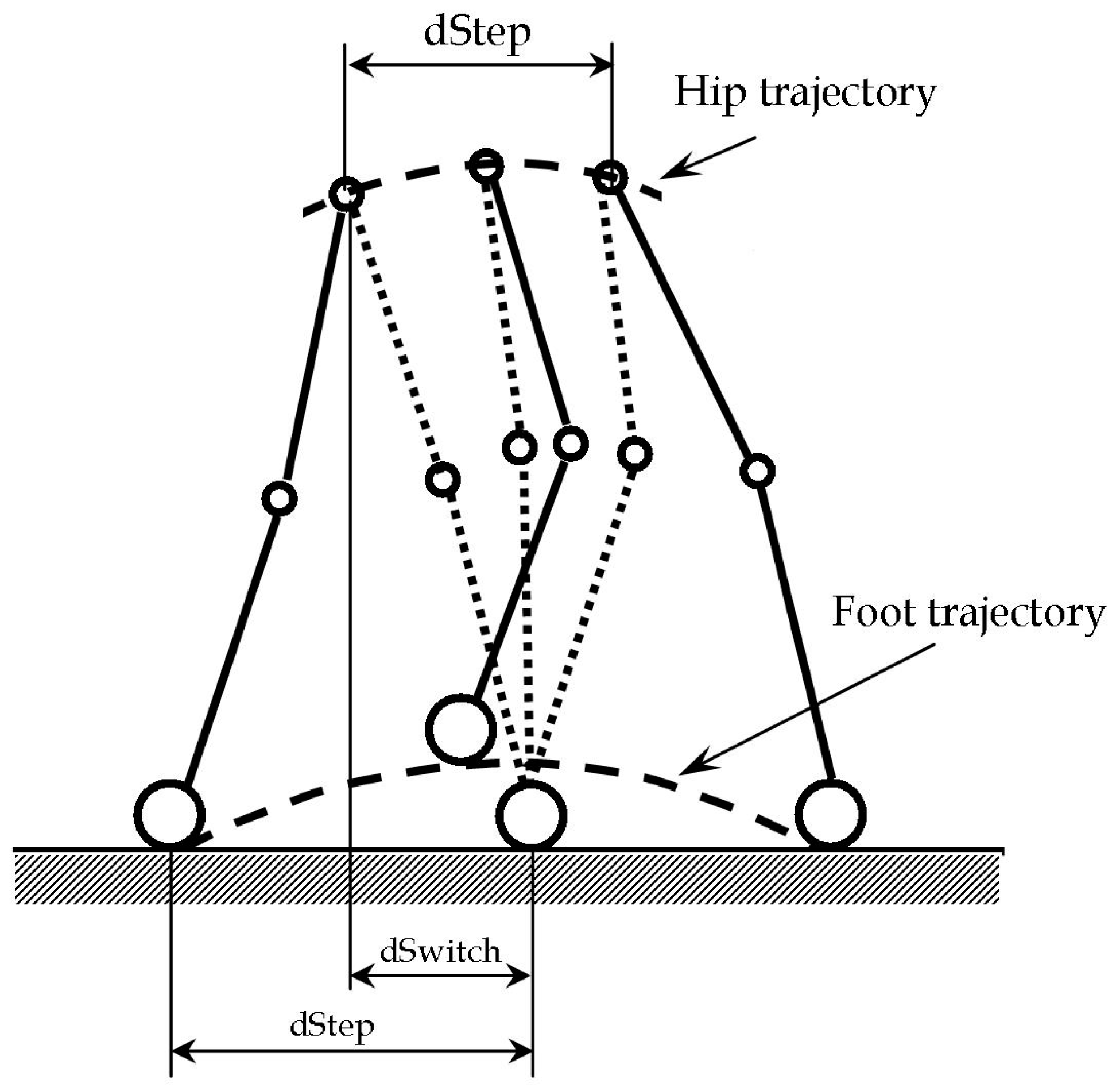
Figure 17 shows a simplified model of the tripod gait in which each set of three legs is modelled as an equivalent leg that can follow a gait planning similar to the one shown in [
37]. The gait is composed of a single support and a double support phase. Gait planning is needed while swinging a leg from a single support to a double support phase.
Figure 17 shows also a model of the swing phase that is basically characterized by two parameters:
- -
dStep, is a distance measured on the X-axis between the support foots. It represents the length of the step.
- -
dSwitch, is the distance, measured along the X-axis, between the projection of hip and the front foot support.
In the double support, both feet are fixed on the ground; accordingly, one can assign the position of the hip. Several strategies are possible, for example, one can choose to maximize the walking step (
dStep) and speed or can choose to minimize energy consumption by keeping the hip at a constant height. As a trade-off solution, one can limit the hip vertical motion to a given percentage of
dStep such as 20% of
dStep. Accordingly, one can define the hip coordinates as
In Equation (25), one can set the initial and final conditions as
combining Equations (25) and (26) one can write
Solving the system for example for
tf = 1 s and
dStep = 25 mm, one can compute the values of coefficients
ax and
bx and
xh coordinate for the hip can be written as
Similarly, for the polynomial function
yh(
t) one can write:
yh(0) = 0;
yh(
tf) = 0;
(0) = 0;
(
tf) = 0 and
Accordingly, one can obtain
The movement is now fully known, as the reference values for the joints of the legs can be obtained through the inverse kinematics equations by substituting Equations (25) and (30) into Equations (2)–(6).
In the single support phase, one of the legs stands on the ground, while the other one is brought forward to complete the step. The point of the hip must travel the distance
dStep. Only a part of this distance will be covered during the single support and the remaining part will be covered in the double support phase. One can define the parameter
Csingle < 1 as expressing the fraction of
dStep that is travelled with in the single support. The values of
Csingle that give the most favorable results have been experimentally found to be in the range of 0.3–0.4, while for humans it is around 0.8 [
37]. The single support begins with the hip in the position
xh0, and ends in the position
xh0 +
Csingle·
dStep, in which the swing foot must be placed on the ground. To determine the intermediate positions, one can define the parameter s where
xh(
t) is the position of the hip along x axis at a given time
t. The parameter s can be used for scaling and synchronizing the trajectory of the hip with the trajectory of the swing foot.
The trajectory (
xsf(
s);
ysf(
s)) of the swing foot can be defined by polynomials third and fourth order as
where
s is obtained by Equation (31). A polynomial of third order for X-axis can specify the boundary conditions (initial and final) in terms of position and speed of the trajectory. A polynomial of fourth order for Y-axis specifies the same boundary conditions, but also can assign the height
h0 of the foot at a given time. This can be useful for avoiding undesired impacts with the ground or for avoiding obstacles. The trajectory is normalized to the parameter s such as proposed in [
38]. This technique of scaling the trajectory is applied since the actual final time
tf at which the foot will rest on the ground is not known a priori. It depends on the dynamic evolution of the system. Assuming
sf = 1, the transition in the point of maximum height
h0 will occur at
s =
sf/2. Accordingly, one can write the boundary conditions as
The origin of the x axis is placed in the support foot, then the swing foot will leave from
xsf(0) = −
dStep then get a
xsf(
tf) = +
dStep. Reasonable value of
h0 for the Cassino Hexapod ranges from 2 to 6 cm. During the single support, one assigns the trajectory expressed in Equation (25), by assigning the parameter
t. For example, if one assigns
dStep = 25 mm,
CSingle = 0
.4,
h0 = 40 mm Equations (25)–(33) lead to
5. Preliminary Validation
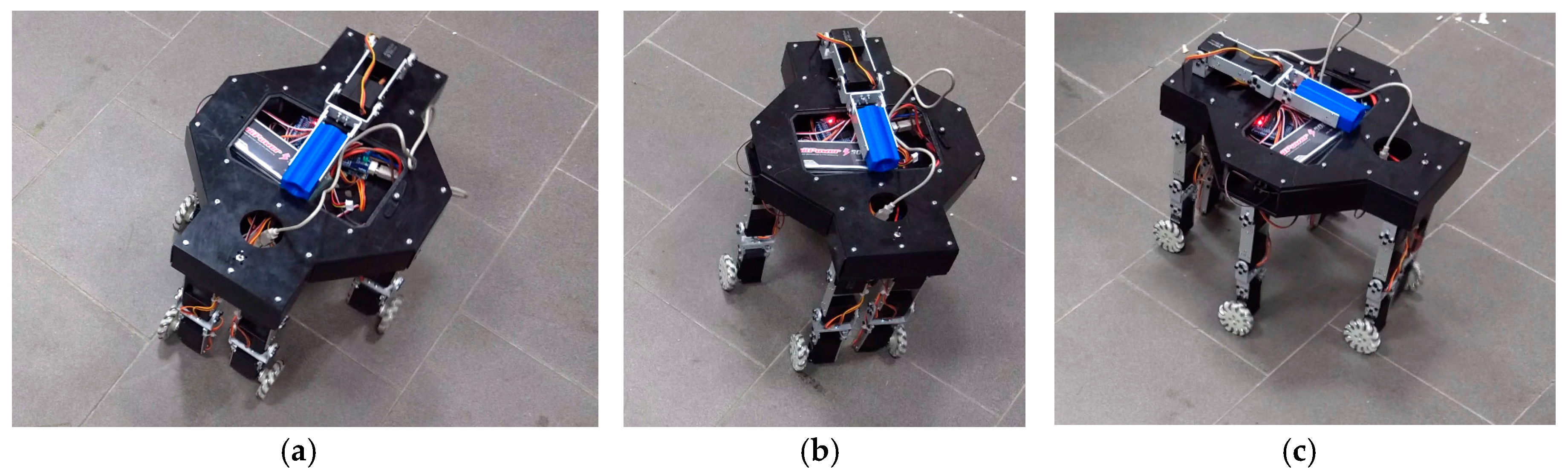
Preliminary tests of the built prototype are currently in progress. For example,
Figure 18 shows several frames that refer to a step climbing strategy. In this experiment, the step height is 50 mm. The robot approaches the step as shown in
Figure 18a. Then, the robot lifts the right forward leg and places it on the step as shown in
Figure 18b. In
Figure 18c the left forward leg is lifted and placed on the step after a forward rolling of wheels. Next step is the lifting of both middle legs together with a forward rolling of wheels, which brings the middle legs in contact with the step as shown in
Figure 18d. This phase is followed by a forward rolling of wheels, which lets the rear legs approach the step as shown in
Figure 18e. The last phases consist in the backward lifting of the rear legs followed by a forward rolling of wheels, which allows the robot to fully overcome the step as shown in
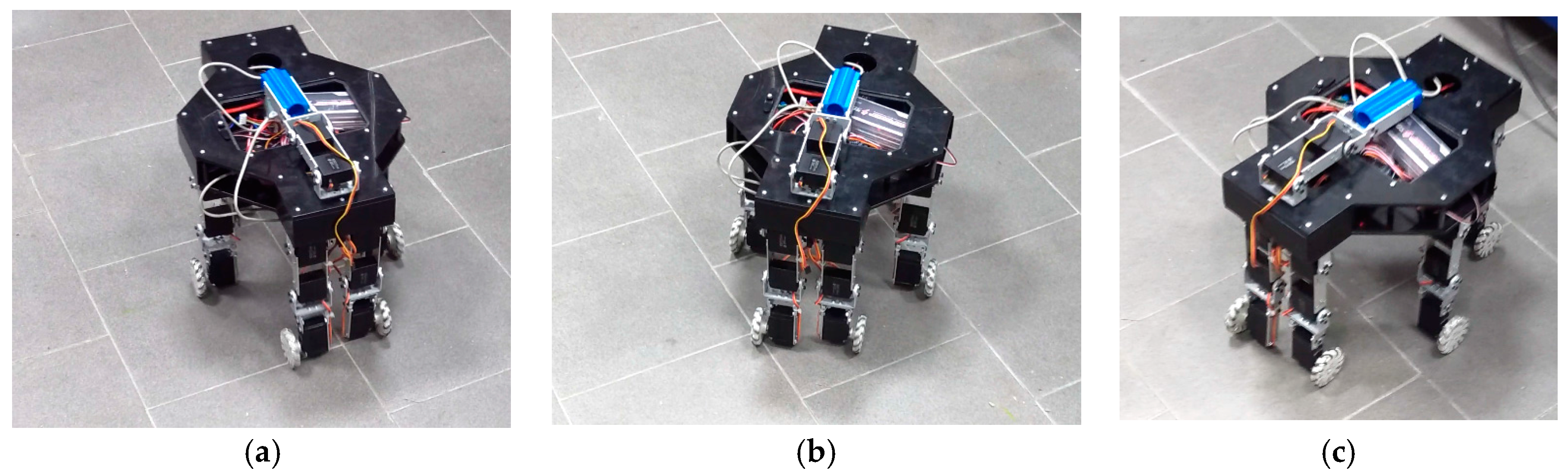
Figure 18f. Further experiments have been carried out to verify the turning ability of Cassino Hexapod III by using omni-wheels operation. Namely, a large radius and small radius turning of 90 degrees have been carried out as shown in
Figure 19 and
Figure 20, respectively. The experiment in
Figure 19 is achieved by rotating the left legs’ wheels at a different speed than the right legs’ wheels. The experiment in
Figure 20 is achieved by counter rotations of omni-wheels, which allow first a horizontal motion of the robot,
Figure 20a followed by a diagonal motion as shown in
Figure 20b, finally a vertical motion is achieved as in
Figure 20c.
Preliminary results show the effectiveness and feasibility of the proposed design solution as well as its gait strategy. In particular, Cassino Hexapod III has successfully achieved preliminary tests in terms of steps overcoming and turning strategies with proper matching with the design specifications as well as with proper operation as based on the developed models and simulations. Future works will be focused on implementation and tests of complex operation tasks according to the proposed specific application. Although on-site operation will require significant time to get the required permissions by the national and local authorities.


