Article

Drive the Drive: From Discrete Motion Plans to Smooth Drivable Trajectories

Centre of Applied Autonomous Sensor Systems (AASS), Örebro University, 70182 Örebro, Sweden
*
Author to whom correspondence should be addressed.
Robotics 2014, 3(4), 400-416; https://doi.org/10.3390/robotics3040400
Submission received: 22 September 2014 / Accepted: 2 December 2014 / Published: 11 December 2014

Abstract

:
Autonomous navigation in real-world industrial environments is a challenging task in many respects. One of the key open challenges is fast planning and execution of trajectories to reach arbitrary target positions and orientations with high accuracy and precision, while taking into account non-holonomic vehicle constraints. In recent years, lattice-based motion planners have been successfully used to generate kinematically and kinodynamically feasible motions for non-holonomic vehicles. However, the discretized nature of these algorithms induces discontinuities in both state and control space of the obtained trajectories, resulting in a mismatch between the achieved and the target end pose of the vehicle. As endpose accuracy is critical for the successful loading and unloading of cargo in typical industrial applications, automatically planned paths have not been widely adopted in commercial AGV systems. The main contribution of this paper is a path smoothing approach, which builds on the output of a lattice-based motion planner to generate smooth drivable trajectories for non-holonomic industrial vehicles. The proposed approach is evaluated in several industrially relevant scenarios and found to be both fast (less than 2 s per vehicle trajectory) and accurate (end-point pose errors below 0.01 m in translation and 0.005 radians in orientation).

Graphical Abstract

1. Introduction

Automatically Guided Vehicles (AGVs) have been deployed in large numbers for industrial intra-logistic tasks. They typically transport payload from a loading to a drop-off location and it is crucial that they drive accurately to given poses. Being able to arrive at a defined pose with high accuracy and precision is a fundamental requirement for AGV systems. It is especially important since most AGV platforms, e.g., forklift trucks [1] or waist-actuated wheel loaders [2], are non-holonomic. Thus, even in cases when an error in the final pose can be reliably detected, it is not possible for the vehicle controller to correct it over a short distance. According to the AGV system provider Kollmorgen [3], the required end pose accuracy for picking up pallets is 0.03 m in position and 1 degree (0.017 radians) in orientation, for example.
In current commercial AGV solutions, all paths need to be defined manually before operation. This is a time-consuming, inflexible and costly procedure, which must be repeated for every new deployment or whenever the area of operation changes. An even more important disadvantage is that paths cannot be changed during operation to respond to obstacles. In order to enable new applications, it is key to replace this inflexible off-line process with on-line motion planning. State-of-the-art motion planners (based either on Rapidly Exploring Random Trees (RRT), Probabilistic Roadmaps (PRM) or state space lattice search) have so far not been demonstrated to generate trajectories that enable AGVs to achieve the required goal pose accuracy for industrial applications. In addition, the trajectories obtained by current planners are not guaranteed to be directly drivable—discontinuities in vehicle controls and within the trajectories are often left untreated and have to be handled by the controller. This is a well known problem which has recently received attention [4,5], but, to-date, no solution has been proposed, which can both guarantee the required accuracy and be used on-line.
The focus of this paper is on on-line motion planning for car-like vehicles given arbitrary end poses. We propose and evaluate a path smoothing approach to improve end pose accuracy obtained with paths generated by a lattice-based motion planner. Of course, the achieved end pose accuracy depends on all navigation subsystems, including motion planning, localization and motion execution. Therefore, we developed a complete navigation system, composed of a lattice-based motion planner, the continuous space path smoother proposed in this paper, a trajectory generator and a model predictive controller. We compare our system against a state-of-the-art commercial AGV solution. For the comparisons in this paper, we rely on a commercial reflector-based localization module.
The contribution of this paper is two-fold. First, we propose a new path smoothing approach that can be used in a complete, on-line navigation system to produce highly accurate motions for car-like vehicles. Our approach does not require a transformation of the input path to a new representation, which is smooth by definition (e.g., splines). Thus, it can directly incorporate state-space constraints in the smoothing process, avoiding the need to verify the path again after smoothing. In our experiments, we show that our approach generates smooth drivable trajectories for arbitrary goal poses in under 2 s (using a single threaded implementation with an i7-2860QM CPU at 2.50 GHz), a fraction of the runtime reported by previous approaches [4]. Second, we describe our complete navigation system and present an extensive experimental evaluation where a non-holonomic vehicle has to sequentially drive to a number of given goal poses (drawn as black arrows in the example depicted in Figure 1). We show the importance of the path smoother and demonstrate that our system can generate and execute smooth paths (see the example in Figure 1 containing paths obtained from a lattice-based motion planner, the corresponding smoothed paths and the actual trajectories driven by the vehicle) with end pose errors comparable to a commercial AGV system based on manually defined paths.
Figure 1. Example of the problem addressed in this paper.
Robotics 03 00400 g001
In Section 2 we present related work on motion planning. We detail our system in Section 3 and present the experimental evaluation in Section 4. Finally, Section 5 concludes with a discussion and presents directions for future research.

2. Related Work

The industry standard for autonomous navigation is to use predefined trajectories that the AGVs follow strictly. The trajectories are either manually defined or learned through teaching-by-demonstration from a human operator [6,7]. Although conceptually simple, this approach has drawbacks such as high deployment costs and lack of flexibility. A change in the configuration of a warehouse or an additional loading point, for instance, require the manual definition of a new set of trajectories. In addition, if an AGV encounters an unforeseen obstacle during operation, it can only employ very simple strategies (typically stopping until the obstacle moves or is removed). To overcome these drawbacks, many different techniques for automatic path and trajectory generation have been proposed in the past decades.
Combinatorial methods are not very well suited in the presence of differential constraints (e.g., kinematic constraints for non-holonomic vehicles) and analytical solutions cannot effectively cope with obstacles [8]. To overcome these problems, sampling-based approaches have been introduced and studied in recent years. In particular, three families of methods are currently widely used: Probabilistic Roadmaps (PRMs) [9], Rapidly-exploring Random Trees (RRTs) [10,11,12] and lattice-based motion planners [13,14]. All sampling-based approaches have been shown to be effective in high-dimensional configuration spaces. Lattice-based motion planners, in particular, combine the strengths of the approaches discussed above with well studied classical AI graph exploration algorithms, such as A * , A R A * and D * L i t e [15]. Differential constraints are incorporated in the search space by means of pre-computed motion primitives, which sample the state space on a regular lattice. The search space is then explored using efficient graph search techniques. However, all sampling-based approaches to non-holonomic motion planning generate paths and trajectories that typically present discontinuities, within the trajectory itself or between the terminal and goal state. This is a known problem and prevents current solutions to achieve the end pose accuracy required by industrial applications. In recent years, several solutions have been suggested for smoothing the trajectories from sampling-based motion planners [4,5]. So far, the methods suggested are computationally too expensive to be used on-line, as smoothing requires time in the order of hundreds or even thousands of seconds [4]. By contrast, our approach is designed to be used on-line and, in the experimental evaluation, we show that the smoothing step usually takes less than two seconds (see Table 1).
A different approach to obtain smooth paths is to start with a set of waypoints, and then to switch to a representation that inherently guarantees continuous curvatures. Popular algorithms take as input a set of waypoints, obtained either automatically [16,17] or by manually driving the vehicle on the desired path [6,7]. Then an optimization procedure is employed, which operates directly on the parameters of the new representation rather than on the waypoints. Common representations are Quintic splines [18], B-splines [17] or clothoids [19,20]. Fitting the new representation to the waypoints in general entails a change of the original path and therefore does not guarantee collision-free paths. Thus, a post-processing step is necessary to check whether the path in the new representation is still collision-free [16,21]. Non-holonomic vehicles have additional constraints on the curvature of the motion, i.e., the maximum steering angle of the vehicle. To guarantee drivable paths, also these constraints require a time-consuming verification after path smoothing by transformation into a different representation.

3. Generating Smooth Trajectories On-Line

We developed our approach to path smoothing and to autonomous navigation to fulfill the stringent requirements for autonomous vehicles in industrial environments. For the definition of these requirements, we relied on the long experience of our industrial partner Kollmorgen, a world leader in providing AGV solutions. Kollmorgen has deployed approximate 15,000 AGVs since 1991 in different industrial settings. According to Kollmorgen, high end pose accuracy is of paramount importance. For safe loading and unloading of pallets, for example, the required end pose accuracy is 0.03 m in position and 1 degree (0.017 radians) in orientation.
In this work, we consider trajectories for AGVs which operate as a fleet for warehouse automation. At the core of the system is a central vehicle coordinator [22], which can directly control the speed of each autonomous vehicle. Thus, the paths and speed profiles of the controlled vehicles have to be computed separately, in order to allow the coordinator to prevent deadlocks. This is a desirable separation whenever multiple AGVs need to be coordinated. For our system, we adopt the three-step approach shown in Figure 2. First, we calculate kinematically drivable paths with a lattice-based motion planner for each vehicle. Then, the path is processed by the path smoother proposed in this paper, resulting in a continuous drivable path. Finally, a trajectory generator associates speed profiles consistent with dynamic and coordination constraints to the smoothed paths and generates the final trajectories that the vehicle controller executes [23].
Figure 2. Overview of the processing steps detailed in Section 3.2, Section 3.3 and Section 3.4 and their connections.
Robotics 03 00400 g002

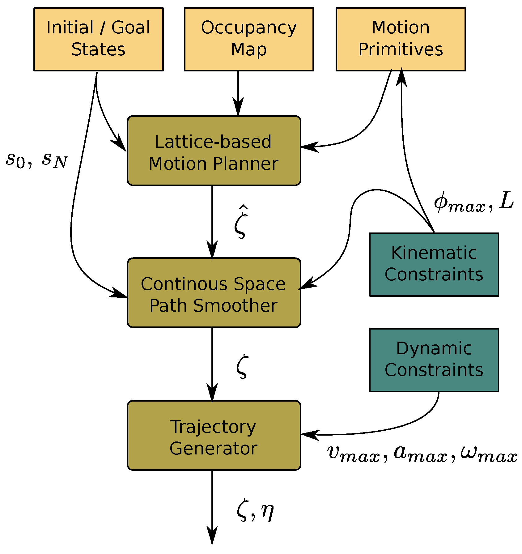
3.1. Problem Formulation

In this paper we consider car-like vehicles (standard trucks, forklifts, etc.) that are commonly found in indoor production sites. The control space u = ( v , ω ) of such vehicles is composed of forward speed v and steering velocity ω. The state space s = ( x , y , θ , ϕ ) consists of all vehicle configurations composed of 2D position ( x , y ) , heading θ and steering angle ϕ. Let ζ and η be sets of N points in state space and control space respectively, defined as:
ζ = { s i } = { ( x i , y i , θ i , ϕ i ) }
η = { u i } = { ( v i , ω i ) }
We assume a fixed time step Δ T = T N ( = 60 m s ) , where T is the time for reaching the goal. The state transition of car-like vehicles s ˙ = f ( s , u , t ) is computed as follows:
x ˙ i = v i cos θ i
y ˙ i = v i sin θ i
θ ˙ i = v i tan ϕ i L
ϕ ˙ i = ω i
where L is the distance between front and back axles.
Given an initial state s ¯ 0 = ( x 0 , y 0 , θ 0 , ϕ 0 ) and a goal state s ¯ N = ( x N , y N , θ N , ϕ N ) for a vehicle, we want to calculate a set of N control points η and the corresponding state points ζ, which can take the vehicle from s ¯ 0 to s ¯ N . A solution to the problem is valid if also additional vehicle-dependent constraints are respected, such as the maximum allowed steering angle ϕ m a x , the maximum steering velocity ω m a x , the maximum forward and reverse velocity v m a x and the maximum acceleration | v ˙ i | a m a x . In our experiments, the x 0 , y 0 and θ 0 components of the start state s 0 are obtained directly from an off-the-shelf localization system, while the steering angle ϕ 0 is taken from absolute encoder readings. The goal state is always assumed to have a steering angle component ϕ N = 0 . See also the overview depicted in Figure 2.

3.2. Lattice-Based Motion Planner

The first step of our approach is a lattice-based motion planner [24], which quickly computes kinematically feasible paths, optimized with respect to a cost function that considers distance traveled and penalizes backwards and turning motions. Given a model of vehicle maneuverability, the intuition behind lattice-based motion planning is to sample the state space in a regular fashion and to constrain the motions of the vehicle to a lattice graph, that is, a graph embedded in a Euclidean space R n which forms a regular tiling [25]. Each vertex of the graph represents a valid configuration of the vehicle, while each edge encodes a motion which respects the non-holonomic constraints of the vehicle. A valid configuration for a vehicle is a four-dimensional vector c = x , y , θ , ϕ , where ( x , y ) lies on a grid of resolution r, θ Θ and ϕ Φ . In the experiments presented in this paper, r is equal to 0 . 2 m, | Θ | = 16 and | Φ | = 1 . In particular, Θ is the set of all the angles in [ 0 , 2 π ) which are multiples of π 8 and Φ = { 0 } , which means that we only consider configurations where the steering angle is equal to 0 with respect to the vehicle itself. This is because reducing the cardinality of Φ reduces the search space and solutions can be calculated quickly. The fact that at this stage the steering angle of the vehicle is assumed to be equal to 0 at the beginning and at the end of every motion is then compensated by our smoother (for the computation times of the planner in our experiments, see Table 1, "Motion planning").
Table 1. Computational time for motion planning and path smoothing (Section 4.3).
Mean (s)Std (s)Max (s)
Motion planning0.1050.0850.680
Path smoothing1.0950.2221.868
The planner uses a set of pre-computed, kinematically feasible motion primitives, which are repeatedly applied to obtain a directed graph which covers the configuration space. Information about the static obstacles in the environment is provided to the planner by an occupancy map and is used to prune the search graph to obtain collision-free paths. The motion primitives are automatically generated to fully capture the mobility of the vehicle and then reduced for efficiency purposes, as described in [26], without compromising the reachability of the configuration space of the vehicle. The graph is then explored using A * , or A R A * [27], one of its most efficient anytime versions, which can provide provable bounds on sub-optimality. Effective heuristic functions [28] and pre-computed vehicle footprints of each motion primitive for fast collision detection are employed to speed up the exploration of the lattice.
Given a start and a goal state ( s 0 , s N ), the motion planner generates an obstacle free, kinematically drivable path ζ ^ , which means that the steering angle constraint - ϕ m a x ϕ ϕ m a x (Equation (6)) is respected. Note that the planner at this stage does not generate the controls for the vehicle. The path ζ ^ , however, brings the vehicle from a discretized start state s ^ 0 to a discretized goal state s ^ N , where s ^ 0 and s ^ N represent the closest states on the lattice to s 0 and s N , respectively. This introduces an error on the order of the lattice discretization. Moreover, ζ ^ is by construction guaranteed to be drivable by the vehicle at a nominal speed and it is C 1 -continuous, but not necessarily C 2 -continuous.

3.3. Continuous Space Path Smoother

The path ζ ^ obtained by the motion planner in the previous section has three distinct problems, which prevent us from directly feeding it to the vehicle controller. First, the start and goal states used by the planner are discretized and do not necessarily correspond to the given initial and end state (see Figure 1). Second, the planner assumes that the steering angle at the start state is always equal to zero, which may not correspond to the actual state of the vehicle. Third, ζ ^ is not necessarily C 2 -continuous, which means that the rate of change of the steering angle of the vehicle can be discontinuous (see Figure 3). While some of these issues can be handled and corrected by the controller, the accuracy of the final vehicle pose with respect to the target pose would be at best on the order of the grid discretization of the planner (as demonstrated in the experiments in Section 4). In order to solve these problems and improve navigation, our approach makes small local modifications to ζ ^ .
Figure 3. Comparison between the original path from the lattice-based motion planner and the smoothed path after applying our continuous space path smoother. (a) paths; (b) steering angles.
Robotics 03 00400 g003
We begin by formulating the above problems as constraints on the states of ζ ^ so as to obtain a set of states and the corresponding control inputs { s i , u i } i = 0 N that satisfy them. First, the start and end states of the modified path need to correspond precisely to the current vehicle state s ¯ 0 and the actual goal state s ¯ N :
s ¯ 0 - s 0 = 0
s ¯ N - s N = 0
These constraints address inaccuracies due to discretization and the assumption of a zero initial steering angle. The additional constraints in Equations (5) – (9) make sure that the path is conform with the kinematic constraints of the vehicle and the constraints on vehicle controls:
s i + 1 = f ( s i , u i ) , i = 1 , , N - 1
ϕ m i n ϕ ϕ m a x
- v m a x v v m a x
- ω m a x ω ω m a x
- a m a x a a m a x
The constraints in Equations (3) – (9) define the set of all possible executable trajectories to bring the vehicle from a given start to a goal state without considering obstacles. An uninformed search through this set of feasible trajectories is a very inefficient way of solving the continuous space motion planning problem in the presence of obstacles. The key to the efficiency that we obtain with the proposed approach is that an uninformed search is not necessary. From the lattice-based motion planner we already have a cost-optimal, obstacle-free path ζ ^ . Although this path generally lies outside the feasible set defined by Equations (3) – (9) we can use it to define a boundary value optimization problem in which we initialize the variables { s i } i = 0 N with the path ζ ^ . We then perform a search for the closest trajectory in the feasible set using a direct multiple shooting method implementation from the ACADO Toolkit [29].
The multiple shooting method [30] assumes that the controls u i are discretized piecewise over time and kept constant during each step Δ T . It utilizes the ordinary differential equations (ODEs) defined above (Equation (2)) to integrate the control value u i over the time Δ T from an initial state value s i to a final state value s i + 1 . In order to obtain a smoothed path, and not only a feasible one, it is important to initialize the control values to a constant value (in the test runs performed for this paper, we initialized the controls as { u i } i = 0 N = ( 0 , 0 ) ). If the initial controls were instead computed based on the initial given path, the obtained path would be feasible but not smoothed, as the turns would be preserved through the process. A multiple shooting method is divided into the following steps: First, a Non-Linear Program is defined so as to include the constraints listed in Equations (5) and (6). The Non-Linear Program is then solved using a Sequential Quadratic Program (SQP). In each SQP iteration the ODEs are recomputed, including their derivatives, which are subsequently used to form a Quadratic Program (QP). The QP is then solved, so as to incrementally update the control values { u i } i = 0 N . This incremental approach limits the amount of control applied, as it can be seen by the reduced changes observable in steering in our experimental evaluation (see Figure 3b). The required number of SQP iterations was typically 3.
One key point of this work is that we formulate the problem as a standard optimization problem. This choice allows us to directly benefit from using the vast amount of freely available optimization tools. We also tried to solve the problem using the single shooting method implementation in ACADO Toolkit [29], and this yielded similar results. Our approach is largely agnostic to a change of the optimization tool since we do not minimize any specific objective function. All the tests presented in this paper, however, were performed using the multiple shooting method.
The output of this optimization phase is a trajectory ( ζ , η ) , including a set of vehicle controls. Since there is no objective which optimizes the speed of the vehicle, the returned control values are only guaranteed to fulfill the kinematic constraints of the vehicle. To obtain the fastest possible trajectory would require to solve a more complex problem, i.e., an Optimal Control Problem, which would be too time consuming. The decoupling of the generation of the control set from the path is further motivated by the fact that the fastest trajectory profile may not necessarily be the optimal one in a multi-robot navigation scenario, as it is common in intra-logistics applications. Our full navigation system employs a centralized coordination scheme [23], whose description is outside the scope of this paper. For the purpose of experimentally evaluating our path smoothing approach, here we rely on a subsequent trajectory generation step (Section 3.4). Because of this decoupling, we can simplify the boundary value optimization problem by delegating the constraints regarding velocities and accelerations (Equations (7) – (9)) to the trajectory generator. In addition, we subsample the number of states and control points N to further reduce the computational time (in our experiments N was 100).
It is important to note that the path smoother changes the path from the motion planner and therefore we cannot guarantee that it is still collision-free. However, the deviation from the input path is very small (see Figure 3). This is because the smoother searches for the closest trajectory in the feasible set starting from the original path. In our current approach we compensate for this limited deviation by assuming an enlarged vehicle footprint during motion planning (width and length were both expanded by 10%). A rigorous way to solve this problem would be to specify boundary conditions on every state during the smoothing step. These constraints would guarantee that the new path is obstacle free. This aspect is left for future work.

3.4. Trajectory Generator

The trajectory generator takes as input the states computed by the path smoother and it works in a similar way as described in [16,31]. More specifically, it assigns the largest possible velocity to each state in the path within the given constraints. The constraints are the boundary conditions with initial and final velocities and limitations on steering velocity, speed and acceleration. The output of this module is a trajectory with a fixed Δ T of 60 ms, used by the controller. In the current implementation we use linear interpolation, which is effective since the distance between interpolation states is small.
In the experimental evaluation the parameters for the maximum velocity, acceleration and steering angle velocity were set to v m a x = 0 . 5 m / s , a m a x = 0 . 2 m / s 2 and ω m a x = 1 r a d / s , respectively.

3.5. Model Predictive Controller

In our vehicle navigation system, we use a Model Predictive Controller (MPC) [23]. The core idea of this type of controllers is to model how the states of the vehicle evolve over a time preview window, given a set of control inputs. The controller then optimizes the control output using an objective function based on the trajectory to follow. In our implementation we use a preview window of 25 control steps and each control step has a duration of 60 ms. The controller gains were set to equally weight heading and distance. This is reflected in the results presented in Figure 4: the heading and distance errors are quantitatively very similar. As the controller is not the main focus of this paper, we use it with default parameters as a “black box” in the experimental evaluation.
Figure 4. Navigation pose accuracy. (a) side distance errors; (b) heading angle errors. The goal IDs refer to Figure 5b. Note that the paths generated by the planner and not processed by the smoother present errors one order of magnitude larger than the ones in the figure and therefore are omitted.
Robotics 03 00400 g004

4. Experimental Evaluation

We evaluated our navigation system using an industrially-relevant vehicle configuration. We deployed an AGV operator training platform from Kollmorgen (Figure 5a) in a small-scale test environment at Örebro University. The vehicle kinematics are the same as those of standard fork lift trucks, with a combined steer and drive wheel. A commercial reflector-based localization solution using 22 reflective beacons was deployed in the test environment. This solution guarantees localization accuracy within less than 1 cm in translation and 0.001 radians in orientation. Using the on-board control system, we can access encoder and localization data and we can set steer and drive commands. All of the remaining components of our system run on a standard laptop with an i7-2860QM CPU at 2.50 GHz.
Figure 5. (a) AGV test platform used in the experiments; (b) Test layout for the comparison of the systems: the blue dots indicate goal poses identified by an ID. The turquoise line in the dots shows the goal headings.
Robotics 03 00400 g005
The overall goal of our experimental evaluation is to demonstrate the accuracy achieved while following the on-line generated trajectories and the reliability of our results. We structure our evaluation in several consecutive parts. First, we compare the controller of our system with the one of the commercial solution over identical, manually crafted trajectories. This set of tests is necessary to guarantee that the results obtained are comparable when using different approaches to path generation and are not biased by different performances at the controller level. The following evaluation step is the most crucial: once established that the two controllers have comparable capabilities, we extract the goal poses from the pre-defined paths and use them as input to our system. This means that we compare our approach, where the paths are automatically generated, with the performance of the commercial system which needs hand coded paths. These experimental runs allow us to demonstrate that our approach can entirely substitute the commercial system without loss of accuracy, thus rendering the time consuming procedure of manual path drawing obsolete. Finally, we test the robustness of our system over randomly generated goal poses and we evaluate the system over longer distances and analyze how the different numbers of control points N used in the path smoother affects the positioning accuracy.

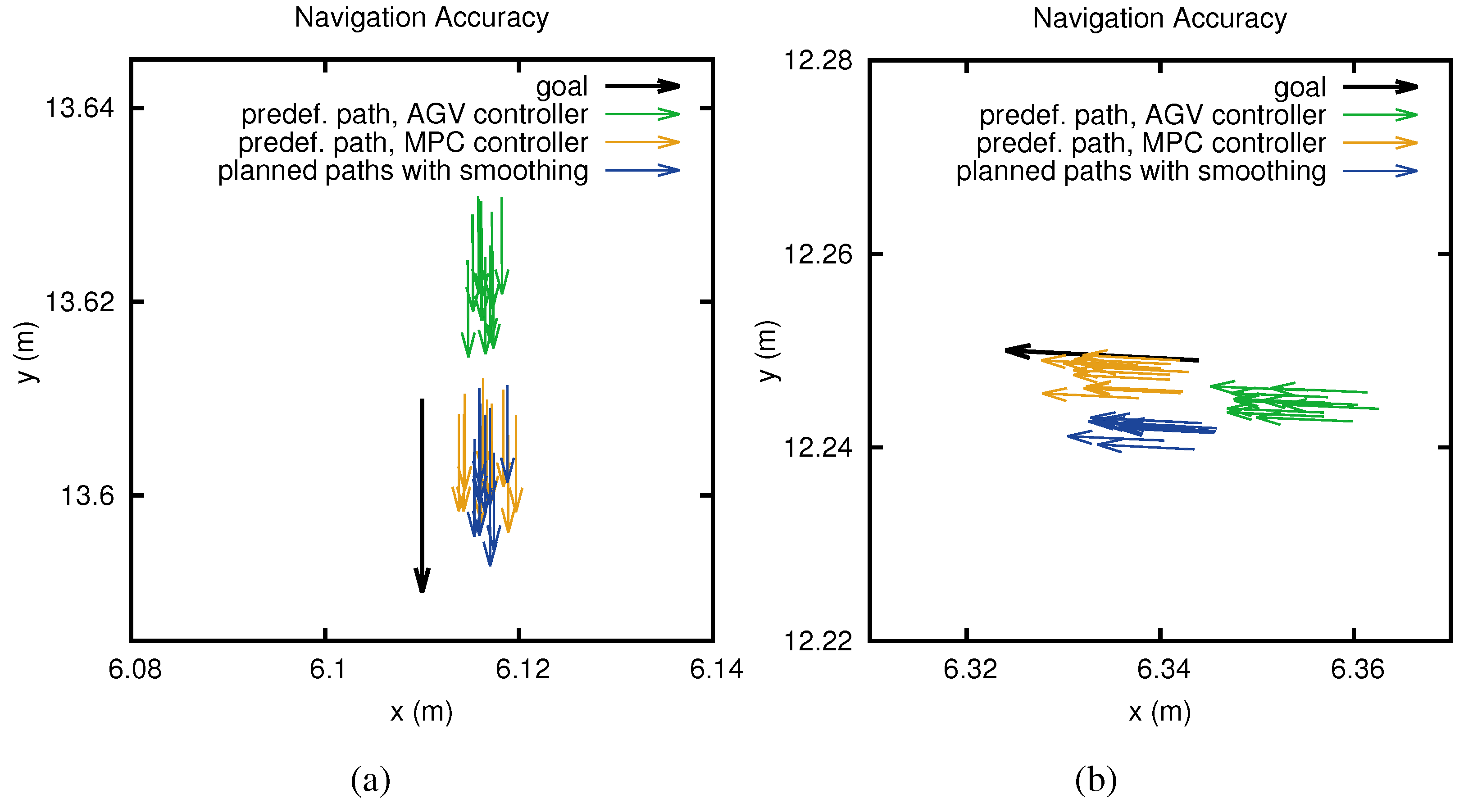
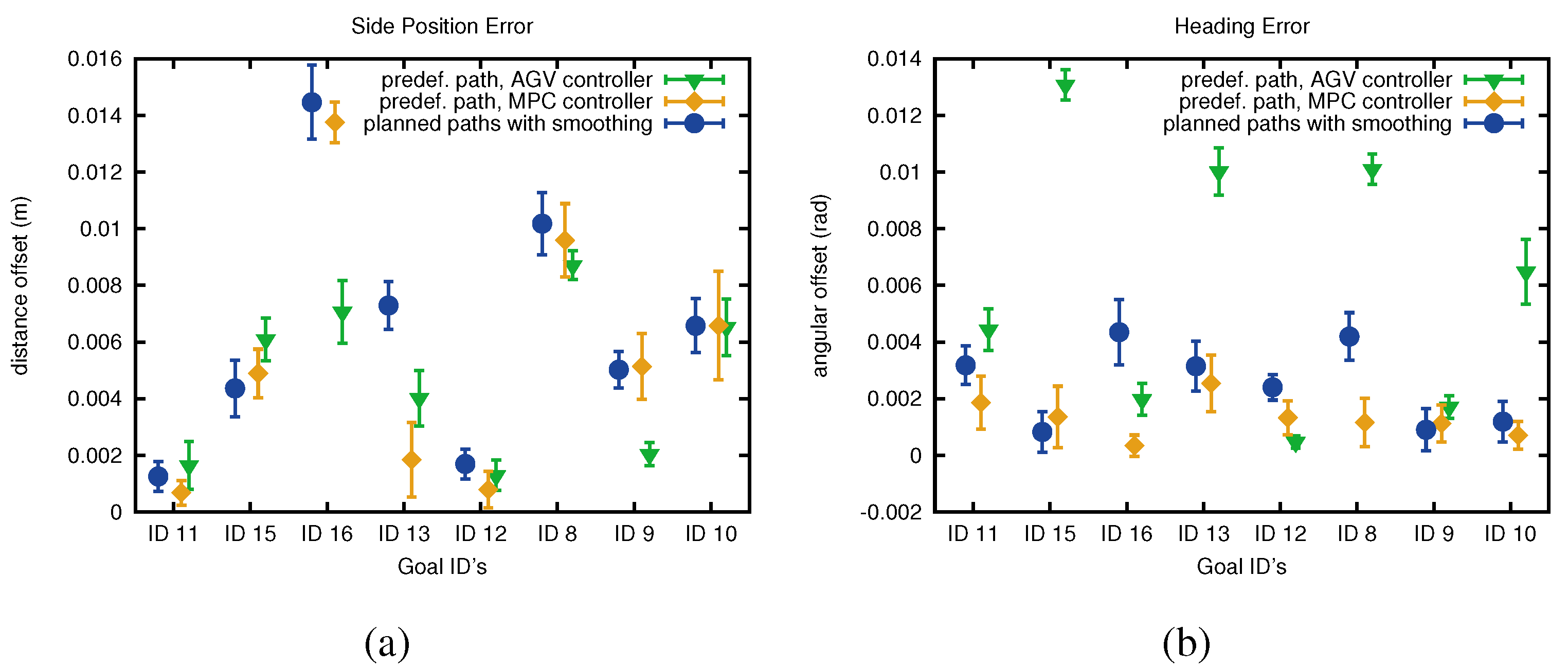
4.1. Controller Comparison

We first created a set of B-spline parametrized trajectories T e v a l (Figure 5b) with an AGV layout drawing tool provided by Kollmorgen. Special care was taken to make these trajectories as smooth as possible. We then used both controllers to follow the trajectories. Each trajectory was executed 10 times. The AGV controller can follow the given trajectories directly, whereas our controller extracts the paths P e v a l from the layout trajectories T e v a l and attaches speed profiles to them, as provided by our trajectory generator (Section 3.4). The tracking performance is shown in the first two lines of Table 2. In particular, we show the performance with respect to the final forward error, side error and heading error, as represented in Figure 6. We separated the errors because, for the controller of a non-holonomic vehicle, it is most difficult to control the heading and the position perpendicular to the direction of motion. For each type of error, we show the results in terms of mean, standard deviation and maximum value obtained in the test runs.
Table 2. Forward and side translation errors and orientation errors
MethodForwardStd (m)Max (m)SideStd (m)Max (m)HeadingStd (rad)Max (rad)
Error (m) Error (m) Error (rad)
predef. path, AGV controller0.01680.00270.02240.00470.00280.00980.00600.00440.0138
predef. path, MPC controller0.00250.00180.00800.00540.00440.01500.00130.00100.0041
planned path with smoothing0.00180.00160.00800.00630.00420.01720.00250.00160.0062
planned path without smoothing0.02730.02990.08860.05210.02110.11160.06210.06020.1783
60 random goals0.00360.00360.02590.00840.00480.02310.00140.00130.0069
Figure 6. The error metrics used in the evaluations.
Robotics 03 00400 g006
The commercial AGV controller has a higher forward error (statistically significant using unpaired t-test; p < 0.0001) which is partly due to an application-specific configuration compared to the MPC used in our system. The heading error is also higher (statistically significant; p < 0.0001) but on the other hand the side error is similar (difference not statistically significant; p = 0.2317). Both controllers are, however, fully capable of tracking the given trajectories.

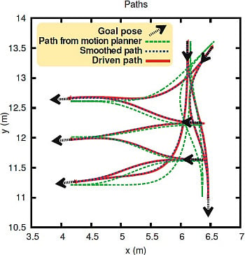
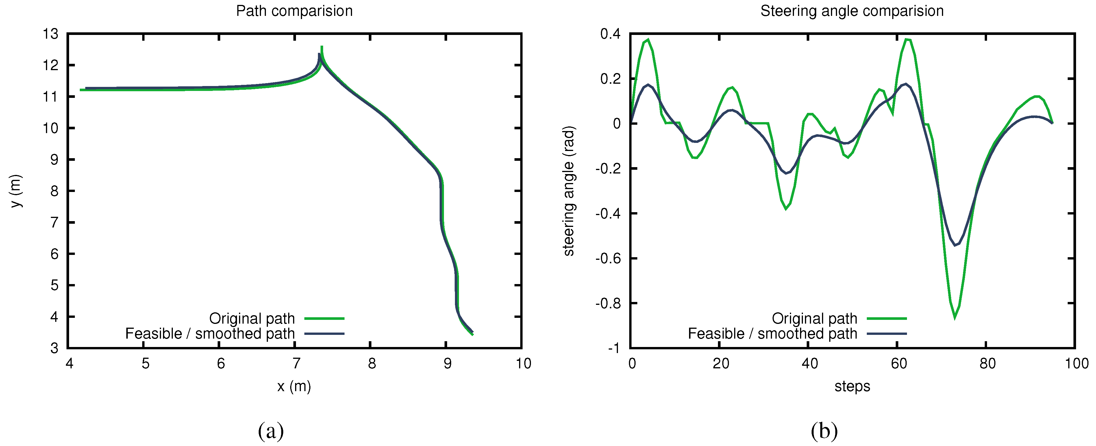
4.2. Path Smoothing of Automatically Generated Paths

After we have established comparable performances of the two controllers, we now compare our complete navigation approach, where paths are automatically generated, with the commercial system, which needs hand coded paths.
We extracted the goal poses from the same paths P e v a l employed in Section 4.1 and used them as targets for our lattice-based motion planner. The output of the planner is passed to the path smoother and then executed by the MPC controller. Table 2 (third and fourth rows) shows results obtained when the motion planner is used with or without path smoothing. Ideally, the automatically generated paths should allow for a comparable pose accuracy as the manually defined paths P e v a l . This is indeed the case in our tests. Please note that in row 4, where the paths are not post-processed by the smoother, the required goal state is set as the last point in the trajectory, thus allowing the controller to correct the state error within the preview window. It can be seen that, in this case, the controller can compensate more effectively for errors in the direction of motion.
These results confirm that our system can produce smooth trajectories which allow very high end pose accuracy, both the heading and the forward error is improved (statistically significant using unpaired t-test; p < 0.0001), whereas the side error is slightly higher (t-test; p = 0.0052). Our approach can entirely substitute the commercial system without loss of accuracy, which makes the time-consuming procedure of manual path definition obsolete. Our results further show the necessity of path smoothing to obtain the required final pose accuracy, which is not possible with state-of-the-art motion planners that need to sample the continuous state space.
A key evaluation metric for AGV systems is their ability to repeatedly reach the same goal pose given a specific path. In an industrial scenario with manually predefined paths, precision is often more important than accuracy since a bias in the end pose can be compensated by adding the corresponding offset to the goal pose. For on-line motion planning, however, the key evaluation metric is end pose accuracy. In either case we are interested in a small variance over the final pose reached. The standard deviation is shown for different goals in Figure 4 and all end poses reached are shown for selected goals in Figure 7a,b. With path smoothing, the end pose variance is small and similar to the one obtained with the commercial system.
Figure 7. End pose accuracy on two different goal poses. (a) goal 10; (b) goal 13.
Robotics 03 00400 g007

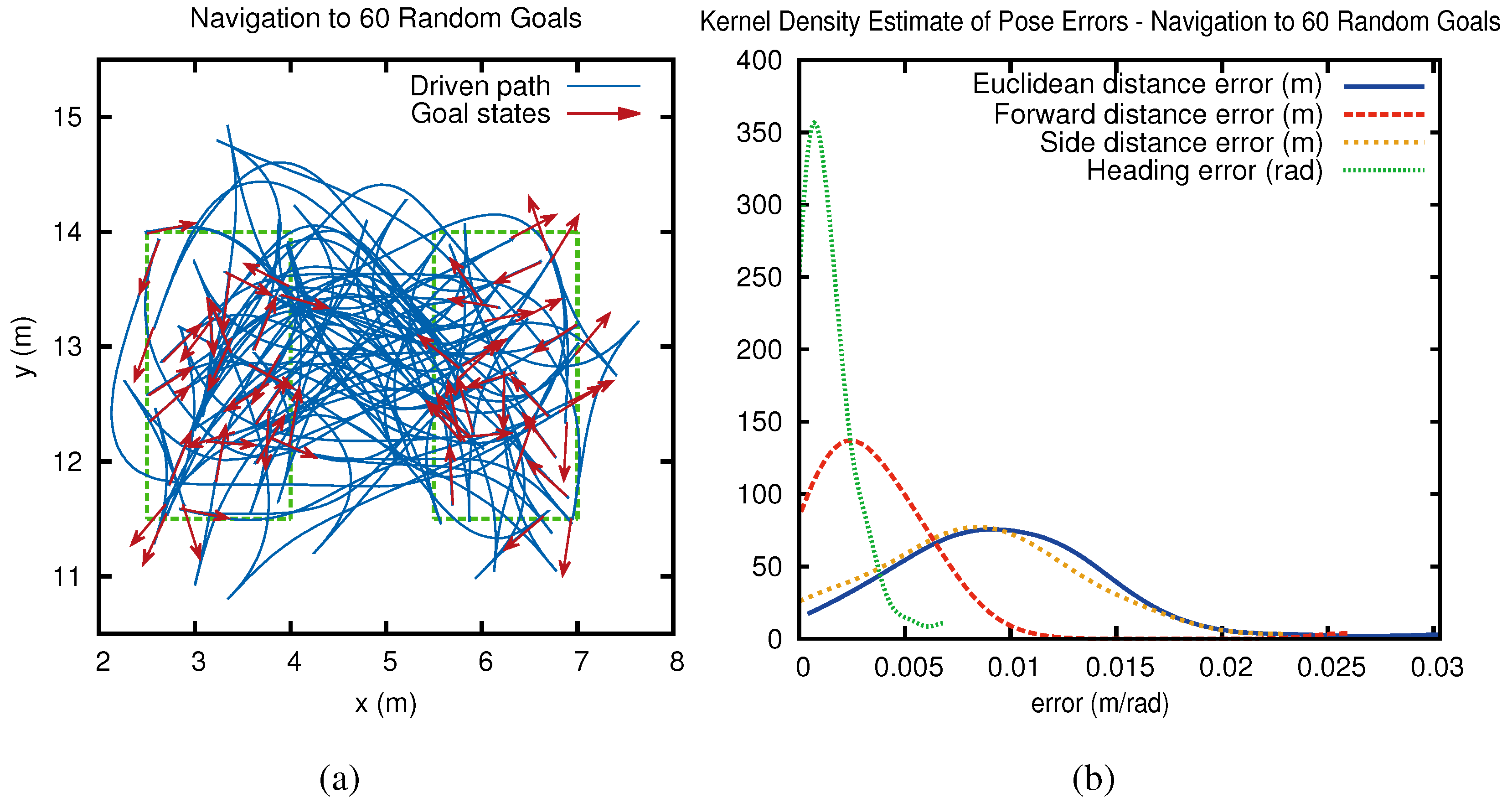
4.3. Evaluation over Randomly Chosen Goals

We further tested the robustness of our system with arbitrary goal poses and over longer distances, by generating a random set of 30 goal poses in two regions of the test environment, marked with dashed lines in Figure 8a. The vehicle traversed back and forth between poses, from one region to the other, for a total of 60 stops. Kernel density estimates of the position and heading errors are plotted in Figure 8b. Side, forward and heading errors are shown in the bottom row of Table 2, while computation times are presented in Table 1 (mean, max and standard deviation).
Figure 8. (a) Path driven while navigating to 60 random goals; (b) Kernel density estimate of corresponding end pose accuracy.
Robotics 03 00400 g008

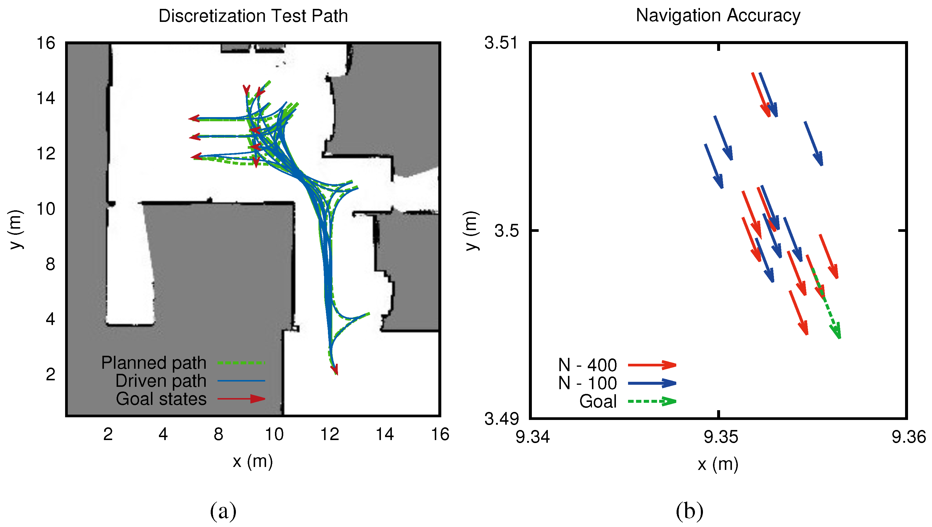
4.4. Evaluation of Discretization Effect on Longer Paths

In order to obtain a path quickly, the number of discretization steps needs to be kept low. However, if the step size is too big, the path smoother will not find paths of the same quality. To evaluate the impact of different numbers of discretization steps, we used again the goal poses shown in Figure 5b, but we interleaved these with an additional goal pose placed further away (see Figure 9a). We compared two different sets of test runs, where the number of discretization steps was set to either 100 or 400. The corresponding end pose accuracy and computation times are shown in Table 3.
Figure 9. (a) Paths and goal poses used in Section 4.4; (b) End pose accuracy of the bottom right goal state.
Robotics 03 00400 g009
Table 3. End pose accuracy and computation time, different discretizations N.
Dist (m)Std (m)Computation Time (s)Std (s)
N = 100 0.01030.00911.52860.1668
N = 400 0.00790.00348.20571.0059
The results shows a minor improvement, but not-statistically significant (performing an unpaired t-test; p = 0.4961), in accuracy (as reported in Figure 9b) at the expense of increased computational costs.

5. Conclusions and Future Work

We have presented a complete navigation system for autonomous, non-holonomic vehicles in industrial settings and we have introduced a novel, fast path smoothing approach, which is applied to the output of a lattice-based motion planner. Lattice-based motion planners, as it is the case with all sampling-based approaches to motion planning, produce motions that present discontinuities which lead to insufficient accuracy and precision in industrial applications. This problem is overcome by our novel approach to path smoothing. Our approach has two major advantages: it can work on-line and uses the same state representation as the motion planner. It could thus directly incorporate state-space constraints in the smoothing process and therefore avoid the need to verify the path again after smoothing. This enables direct initialization of the path smoother with the automatically generated obstacle-free paths. Curvature checks on the final path are not necessary and we can directly include additional constraints in the optimization process. This opens up new possibilities to constrain the vehicle when it approaches the goal state. Constraining steering more in the last segments of the path could, for instance, improve pose accuracy even further. This, however, is left for future work. Another interesting avenue for further investigation will be to apply our approach to other planners, RRT- and PRM-based, to ascertain the generalizability of our methodology.
We have also presented an extensive experimental evaluation of our complete system and of all its major components. In the evaluation, we have compared our system with a state-of-the-art commercial solution, obtaining comparable results with respect to accuracy and precision. However, our system has the advantage that it can automatically plan trajectories on-line, instead of relying on expensive manual drawing.

Acknowledgments

This work was supported by the Swedish Knowledge Foundation (KKS) under projects: SAVIE, SAUNA and Semantic Robots.

Author Contributions

Henrik Andreasson worked on the main part of the experimental evaluation together with Jari Saarinen. The implementation was done by Henrik Andreasson with assistance of Marcello Cirillo and Todor Stoyanov. Henrik Andreasson, Jari Saarinen, Marcello Cirillo, Todor Stoyanov and Achim J. Lilienthal all contributed to the preparation of the manuscript. All listed authors discussed and approved the final manuscript.

Conflicts of Interest

The authors declare no conflict of interest.

References

  1. Bouguerra, A.; Andreasson, H.; Lilienthal, A.J.; Åstrand, B.; Rögnvaldsson, T. MALTA: A System of Multiple Autonomous Trucks for Load Transportation. In Proceedings of the European Conference on Mobile Robots (ECMR), Mlini/Dubrovnik, Croatia, 23–25 September 2009.
  2. Magnusson, M.; Almqvist, H. Consistent Pile-Shape Quantification for Autonomous Wheel Loaders. In Proceedings of the IEEE/RSJ International Conference on Intelligent Robots and Systems (IROS), San Francisco, CA, USA, 25–30 September 2011.
  3. Kollmorgen web page. Available online: http:www.kollmorgen.com (accessed on 10 December 2014).
  4. Cheng, P.; Frazzoli, E.; LaValle, S. Improving the performance of sampling-based motion planning with symmetry-based gap reduction. IEEE Trans. Robot. 2008, 24, 488–494. [Google Scholar] [CrossRef]
  5. Seiler, K.M.; Singh, S.P.; Sukkarieh, S.; Durrant-Whyte, H. Using Lie group symmetries for fast corrective motion planning. Int. J. Robot. Res. 2012, 31, 151–166. [Google Scholar] [CrossRef]
  6. Hellstrom, T.; Ringdahl, O. Follow the past: A path-tracking algorithm for autonomous vehicles. Int. J. Veh. Auton. Syst. 2006, 4, 216–224. [Google Scholar] [CrossRef]
  7. Marshall, J.; Barfoot, T.; Larsson, J. Autonomous underground tramming for center-articulated vehicles. J. Field Robot. 2008, 25, 400–421. [Google Scholar] [CrossRef]
  8. LaValle, S.M. Planning Algorithms; Cambridge University Press: Cambridge, UK, 2006. [Google Scholar]
  9. Kavraki, L.; Svestka, P.; Latombe, J.; Overmars, M. Probabilistic roadmaps for path planning in high-dimensional configuration spaces. IEEE Trans. Robot. Autom. 1996, 12, 566–580. [Google Scholar] [CrossRef]
  10. LaValle, S.M. Rapidly-Exploring Random Trees: A New Tool for Path Planning; Technical Report, TR 98-11; Computer Science Department, Iowa State University: USA, 1998. [Google Scholar]
  11. Karaman, S.; Frazzoli, E. Sampling-based algorithms for optimal motion planning. Int. J. Robot. Res. 2011, 30, 846–894. [Google Scholar] [CrossRef]
  12. Islam, F.; Nasir, J.; Malik, U.; Ayaz, Y.; Hasan, O. RRT*-Smart: Rapid convergence implementation of RRT* towards optimal solution. In Proceedings of the International Conference on Mechatronics and Automation (ICMA), Chengdu, China, 5–8 August 2012.
  13. Ferguson, D.; Likhachev, M. Efficiently using cost maps for planning complex maneuvers. In Proceedings of the ICRA Workshop on Planning with Cost Maps, Pasadena, California, USA, 19–23 May 2008.
  14. Pivtoraiko, M.; Kelly, A. Fast and Feasible Deliberative Motion Planner for Dynamic Environments. In Proceedings of the ICRA Workshop on Safe Navigation in Open and Dynamic Environments: Application to Autonomous Vehicles, Kobe, Japan, 12–17 May 2009.
  15. Koenig, S.; Likhachev, M. D* Lite. In Proceedings of the National Conference on Artificial Intelligence (AAAI), Edmonton, Alberta, Canada, 28 July–1 August 2002.
  16. Lau, B.; Sprunk, C.; Burgard, W. Kinodynamic Motion Planning for Mobile Robots Using Splines. In Proceedings of the IEEE/RSJ International Conference on Intelligent Robots and Systems (IROS), St.Louis, MO, USA, 11–15 October 2009.
  17. Walther, M.; Steinhaus, P.; Dillmann, R. Using B-Splines for Mobile Robot Path Representation and Motion Control. In Proceedings of the European Conference on Mobile Robots (ECMR), Ancona, Italy, 7–10 September 2005.
  18. Sprunk, C.; Lau, B.; Burgard, W. Improved Non-linear Spline Fitting for Teaching Trajectories to Mobile Robots. In Proceedings of the IEEE International Conference on Robotics and Automation (ICRA), St. Paul, MN, USA, 14–18 May 2012.
  19. Wilde, D.K. Computing clothoid segments for trajectory generation. In Proceedings of the IEEE/RSJ International Conference on Intelligent Robots and Systems (IROS), St. Louis, MO, USA, 11–15 October 2009.
  20. Brezak, M.; Petrovic, I. Path Smoothing Using Clothoids for Differential Drive Mobile Robots. In Proceedings of the 18th IFAC World Congress, Milano, Italy, 28 August–2 September 2011.
  21. Sprunk, C.; Lau, B.; Pfaff, P.; Burgard, W. Online Generation of Kinodynamic Trajectories for Non-Circular Omnidirectional Robots. In Proceedings of the IEEE International Conference on Robotics and Automation (ICRA), Shanghai, China, 9–13 May 2011.
  22. Cirillo, M.; Uras, T.; Koenig, S.; Andreasson, H.; Pecora, F. Integrated Motion Planning and Coordination for Industrial Vehicles. In Proceedings of the 24th International Conference on Automated Planning and Scheduling, Portsmouth, NH, USA, 21–26 June 2014.
  23. Pecora, F.; Cirillo, M.; Dimitrov, D. On Mission-Dependent Coordination of Multiple Vehicles under Spatial and Temporal Constraints. In Proceedings of the IEEE/RSJ International Conference on Intelligent Robots and Systems (IROS), Algarve, Portugal, 7–12 October 2012.
  24. Cirillo, M.; Uras, T.; Koenig, S. A Lattice-Based Approach to Multi-Robot Motion Planning for Non-Holonomic Vehicles. In Proceedings of the IEEE/RSJ International Conference on Intelligent Robots and Systems (IROS), Chicago, IL, USA, 14–18 September 2014.
  25. Pivtoraiko, M.; Knepper, R.A.; Kelly, A. Differentially Constrained Mobile Robot Motion Planning in State Lattices. J. Field Robot. 2009, 26, 308–333. [Google Scholar] [CrossRef]
  26. Pivtoraiko, M.; Kelly, A. Kinodynamic motion planning with state lattice motion primitives. In Proceedings of the IEEE/RSJ International Conference on Intelligent Robots and Systems (IROS), San Francisco, CA, USA, 25–30 September 2011.
  27. Likhachev, M.; Gordon, G.; Thrun, S. ARA*: Anytime A* with provable bounds on sub-optimality. Adv. Neural Inf. Process. Syst. 2003, 16, 767–774. [Google Scholar]
  28. Knepper, R.A.; Kelly, A. High Performance State Lattice Planning Using Heuristic Look-Up Tables. In Proceedings of the IEEE/RSJ International Conference on Intelligent Robots and Systems (IROS), Beijing, China, 9–15 October 2006.
  29. Houska, B.; Ferreau, H.; Diehl, M. ACADO Toolkit—An Open Source Framework for Automatic Control and Dynamic Optimization. Optim. Control Appl. Methods 2011, 32, 298–312. [Google Scholar] [CrossRef]
  30. Bock, H.; Plitt, K. A Multiple Shooting algorithm for direct solution of optimal control problems. In Proceedings of the 9th IFAC World Congress, Budapest, Hungary, 2–6 July 1984; pp. 242–247.
  31. Munoz, V.F.; Ollero, A. Smooth trajectory planning method for mobile robots. In Proceedings of the Conference on Computational Engineering in Systems Applications, Lille, France, 9–12 July 1996.

