Article

The Role of Visibility in Pursuit/Evasion Games

1
Department of Electrical and Computer Engineering, Aristotle University, GR 54248, Thessaloniki, Greece
2
Laboratoire J. A. Dieudonné, UMR CNRS-UNS No 7351, Université de Nice Sophia-Antipolis, Parc Valrose 06108 Nice Cedex 2, France
3
Department of Mathematics, Ryerson University, 350 Victoria St., Toronto, ON, M5B 2K3, Canada
*
Author to whom correspondence should be addressed.
Robotics 2014, 3(4), 371-399; https://doi.org/10.3390/robotics3040371
Submission received: 3 September 2014 / Revised: 6 November 2014 / Accepted: 26 November 2014 / Published: 8 December 2014
(This article belongs to the Special Issue Coordination of Robotic Systems)

Abstract

:
The cops-and-robber (CR) game has been used in mobile robotics as a discretized model (played on a graph G) of pursuit/evasion problems. The “classic” CR version is a perfect information game: the cops’ (pursuer’s) location is always known to the robber (evader) and vice versa. Many variants of the classic game can be defined: the robber can be invisible and also the robber can be either adversarial (tries to avoid capture) or drunk (performs a random walk). Furthermore, the cops and robber can reside in either nodes or edges of G. Several of these variants are relevant as models or robotic pursuit/evasion. In this paper, we first define carefully several of the variants mentioned above and related quantities such as the cop number and the capture time. Then we introduce and study the cost of visibility (COV), a quantitative measure of the increase in difficulty (from the cops’ point of view) when the robber is invisible. In addition to our theoretical results, we present algorithms which can be used to compute capture times and COV of graphs which are analytically intractable. Finally, we present the results of applying these algorithms to the numerical computation of COV.

1. Introduction

Pursuit/evasion (PE) and related problems (search, tracking, surveillance) have been the subject of extensive research in the last fifty years and much of this research is connected to mobile robotics [1]. When the environment is represented by a graph (for instance, a floorplan can be modeled as a graph, with nodes corresponding to rooms and edges corresponding to doors; similarly, a maze can be represented by a graph with edges corresponding to tunnels and nodes corresponding to intersections), the original PE problem is reduced to a graph game played between the pursuers and the evader.
In the current paper, inspired by Isler and Karnad’s recent work [2], we study the role of information in cops-and-robber (CR) games, an important version of graph-based PE. By “information” we mean specifically the players’ location. For example, we expect that when the cops know the robber’s location they can do better than when the robber is “invisible”. Our goal is to make precise the term “better”.
Reviews of the graph theoretic CR literature appear in [3,4,5]. In the “classical” CR variant [6] it is assumed that the cops always know the robber’s location and vice versa. The “invisible” variant, in which the cops cannot see the robber (but the robber always sees the cops) has received less attention in the graph theoretic literature; among the few papers which treat this case we mention [2,7,8,9] and also [10] in which both cops and robber are invisible.
Both the visible and invisible CR variants are natural models for discretized robotic PE problems; the connection has been noted and exploited relatively recently [2,8,11]. If it is further assumed that the robber is not actively trying to avoid capture (the case of drunk robber) we obtain a one-player graph game; this model has been used quite often in mobile robotics [12,13,14,15,16] and especially (when assuming random robber movement) in publications such as [17,18,19,20,21], which utilize partially observable Markov decision processes (POMDP, [22,23,24]). For a more general overview of pursuit/evasion and search problems in robotics, the reader is referred to [1]; some of the works cited in this paper provide a useful background to the current paper. Finally, several related works have also been published in the Distributed Algorithms community [25,26,27].
This paper is structured as follows. In Section 2 we present preliminary material, notation and the definition of the “classical” CR game; we also introduce several node and edge CR variants. In Section 3 we define rigorously the cop number and capture time for the classical CR game and the previously introduced CR variants. In Section 4 we study the cost of visibility (COV). In Section 5 we present algorithms which compute capture time and optimal strategies for several CR variants. In Section 6 we further study COV using computational experiments. Finally, in Section 7 we summarize and present our conclusions.

2. Preliminaries

2.1. Notation

  • We use the following notations for sets: N denotes 1 , 2 , ; N 0 denotes 0 , 1 , 2 , ; K denotes 1 , , K ; A B = x : x A , x B ; A denotes the cardinality of A (i.e., the number of its elements).
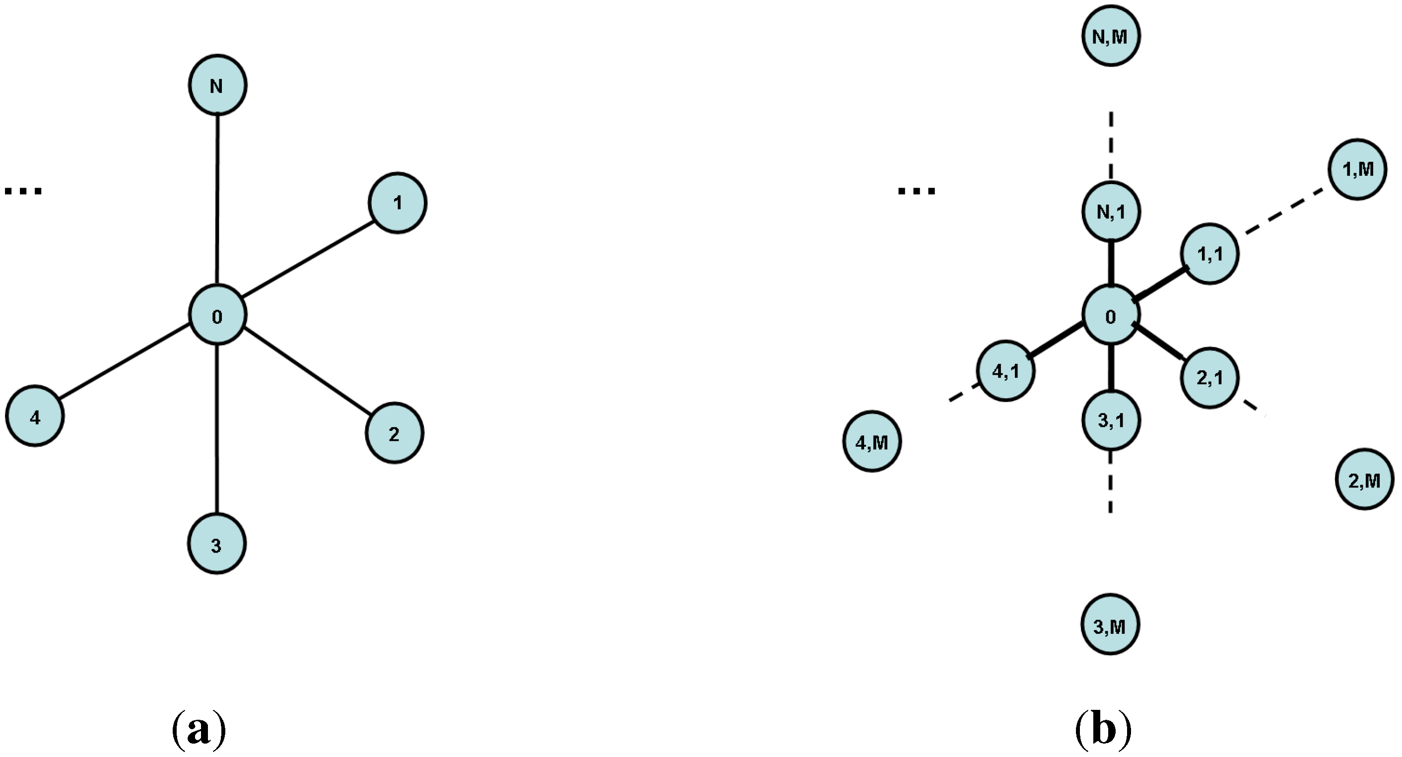
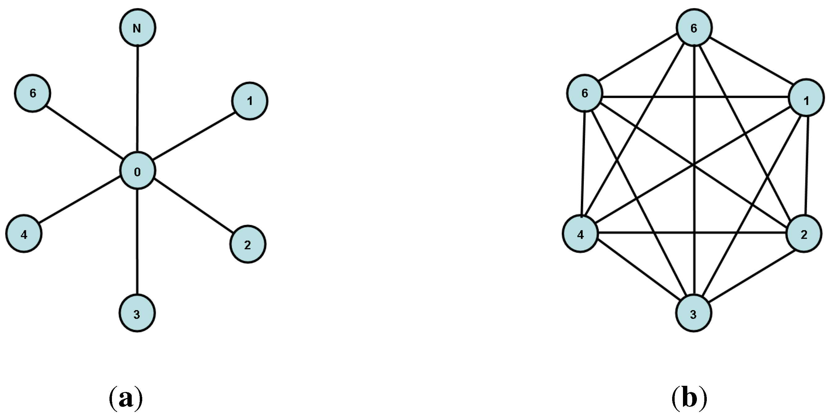
  • A graph G = ( V , E ) consists of a node set V and an edge set E, where every e E has the form e = x , y V . In other words, we are concerned with finite, undirected, simple graphs; in addition we will always assume that G is connected and that G contains n nodes: V = n . Furthermore, we will assume, without loss of generality, that the node set is V = 1 , 2 , , n . We let V K = V × V × × V K times . We also define V D 2 V 2 by V D 2 = { ( x , x ) : x V } (it is the set of “diagonal” node pairs).
  • A directed graph (digraph) G = ( V , E ) consists of a node set V and an edge set E, where every e E has the form e = x , y V × V . In other words, the edges of a digraph are ordered pairs.
  • In graphs, the (open) neighborhood of some x V is N x = y : x , y E ; in digraphs it is N x = y : x , y E . In both cases, the closed neighborhood of x is N x = N x x .
  • Given a graph G = V , E , its line graph L G = V , E is defined as follows: the node set is V = E , i.e., it has one node for every edge of G; the edge set is defined by having the nodes u , v , x , y V connected by an edge u , v , x , y if and only if u , v x , y = 1 (i.e., if the original edges of G are adjacent).
  • We will write f n = o g n if and only if lim n f n g n = 0 . Note that in this asymptotic notation n denotes the parameter with respect to which asymptotics are considered. So in later sections we will write o n , o M etc.

2.2. The CR Game Family

The “classical” CR game can be described as follows. Player C controls K cops (with K 1 ) and player R controls a single robber. Cops and robber are moved along the edges of a graph G = V , E in discrete time steps t N 0 . At time t, the robber’s location is Y t V and the cops’ locations are X t = ( X t 1 , X t 2 , , X t K ) V K (for t N 0 and k K ). The game is played in turns; in the 0-th turn first C places the cops on nodes of the graph and then R places the robber; in the t-th turn, for t > 0 , first C moves the cops to X t and then R moves the robber to Y t . Two types of moves are allowed: (a) sliding along a single edge and (b) staying in place; in other words, for all t and k, either { X t 1 k , X t k } E or X t 1 k = X t k ; similarly, { Y t 1 , Y t } E or Y t 1 = Y t . The cops win if they capture the robber, i.e., if there exist t N 0 and k K such that Y t = X t k ; the robber wins if for all t N 0 and k K we have Y t X t k . In what follows we will describe these eventualities by the following “shorthand notation”: Y t X t and Y t X t (i.e., in this notation we consider X t as a set of cop positions).
In the classical game both C and R are adversarial: C plays to effect capture and R plays to avoid it. But there also exist “drunk robber” versions, in which the robber simply performs a random walk on G such that, for all u , v V we have
Pr Y 0 = u = 1 n and Pr Y t + 1 = u | Y t = v = 1 N v if and only if u N ( v ) 0 otherwise
In this case we can say that no R player is present (or, following a common formulation, we can say that the R player is “Nature”).
If an R player exists, the cops’ locations are always known to him; on the other hand, the robber can be either visible (his location is known to C) or invisible (his location is unknown). Hence we have four different CR variants, as detailed in the following Table 1.
Table 1. Four variants of the CR game.
Adversarial Visible Robberav-CR
Adversarial Invisible Robberai-CR
Drunk Visible Robberdv-CR
Drunk Invisible Robberdi-CR
In all of the above CR variants both cops and robber move from node to node. This is a good model for entities (e.g., robots) which move from room to room in an indoor environment. There also exist cases (for example moving in a maze or a road network) where it makes more sense to assume that both cops and robber move from edge to edge. We will call the classical version of the edge CR game edge av-CR; it has attracted attention only recently [28]. Edge ai-CR, dv-CR and di-CR variants are also possible, in analogy to the node versions listed in the Table. Each of these cases can be reduced to the corresponding node variant, with the edge game taking place on the line graph L G of G.

3. Cop Number and Capture Time

Two graph parameters which can be obtained from the av-CR game are the cop number and the capture time. In this section we will define these quantities in game theoretic terms (while this approach is not common in the CR literature, we believe it offers certain advantages in clarity of presentation) and also consider their extensions to other CR variants. Before examining each of these CR variants in detail, let us mention a particular modification which we will apply to all of them. Namely, we assume that (every variant of) the CR game is played for an infinite number of rounds. This is obviously the case if the robber is never captured; but we also assume that, in case the robber is captured at some time t * , the game continues for t { t * + 1 , t * + 2 , } with the following restriction: for all t t * , we have Y t = X t k * (where k * is the number of cop who effected the capture). This modification facilitates the game theoretic analysis presented in the sequel; intuitively, it implies that after capture, the k * -th cop forces the robber to “follow” him.

3.1. The Node av-CR Game

We will define cop number and capture time in game theoretic terms. To this end we must first define histories and strategies.
A particular instance of the CR game can be fully described by the sequence of cops and robber locations; these locations are fully determined by the C and R moves. So, if we let x t V K (resp. y t V ) denote the nodes into which C (resp. R) places the cops (resp. the robber) at time t, then a history is a sequence x 0 y 0 x 1 y 1 . Such a sequence can have finite or infinite length; we denote the set of all finite length histories by H * K ; note that there exists an infinite number of finite length sequences. By convention H * K also includes the zero-length or null history, which is the empty sequence (this corresponds to the beginning of the game, when neither player has made a move, just before C places the cops on G), denoted by λ. Finally, we denote the set of all infinite length histories by H K .
Since both cops and robber are visible and the players move sequentially, av-CR is a game of perfect information; in such a game C loses nothing by limiting himself to pure (i.e., deterministic) strategies [29]. A pure cop strategy is a function s C : H * K V K ; a pure robber strategy is a function s R : H * K V . In both cases the idea is that, given a finite length history, the strategy produces the next cop or robber move (note the dependence on K, the number of cops); for example, when the robber strategy s R receives the input x 0 , it will produce the output y 0 = s R x 0 ; when it receives x 0 y 0 x 1 , it will produce y 1 = s R x 0 y 0 x 1 and so on. We will denote the set of all legal cop strategies by S C K and the set of all legal robber strategies by S R K ; a strategy is “legal” if it only provides moves which respect the CR game rules. The set S ˜ C K S C K (resp. S ˜ R K S R K ) is the set of memoryless legal cop (resp. robber) strategies, i.e., strategies which only depend only on the current cops and robber positions; we will denote the memoryless strategies by Greek letters, e.g., σ C , σ R etc. In other words
σ C S ˜ C K t : x t + 1 = σ C x 0 y 0 . x t y t = σ C x t y t σ R S ˜ R K t : y t + 1 = σ R x 0 y 0 . x t y t x t + 1 = σ R y t x t + 1
It seems intuitively obvious that both C and R lose nothing by playing with memoryless strategies (i.e., computing their next moves based on the current position of the game, not on its entire history). This is true but requires a proof. One approach to this proof is furnished in [30,31]. But we will present another proof by recognizing that the CR game belongs to the extensively researched family of reachability games [32,33].
A reachability game is played by two players (Player 0 and Player 1) on a digraph G ¯ = V ¯ , E ¯ ; each node v V ¯ is a position and each edge is a move; i.e., the game moves from node to node (position) along the edges of the digraph. The game is described by the tuple V ¯ 0 , V ¯ 1 , E ¯ , F ¯ , where V ¯ 0 V ¯ 1 = V ¯ , V ¯ 0 V ¯ 1 = and F ¯ V ¯ . For i 0 , 1 , V ¯ i is the set of positions (nodes) from which the i-th Player makes the next move; the game terminates with a win for Player 0 if and only if a move takes place into a node v F ¯ (the target set of Player 0); if this never happens, Player 1 wins. Here is a more intuitive description of the game: each move consists in sliding a token from one digraph node to another, along an edge; the i-th player slides the token if and only if it is currently located on a node v V ¯ i ( i 0 , 1 ); Player 0 wins if and only if the token goes into a node u F ¯ ; otherwise Player 1 wins. The following is well known [32,33].
Theorem 1. Let V ¯ 0 , V ¯ 1 , E ¯ , F ¯ be a reachability game on the digraph D ¯ = V ¯ , E ¯ . Then V ¯ can be partitioned into two sets W ¯ 0 and W ¯ 1 such that (for i 0 , 1 ) player i has a memoryless strategy σ i which is winning whenever the game starts in u W ¯ i .
We can convert the av-CR game with K cops to an equivalent reachability game which is played on the CR game digraph. In this digraph every node corresponds to a position of the original CR game; a (directed) edge from node u to node v indicates that it is possible to get from position u to position v in a single move. The CR game digraph has three types of nodes.
  • Nodes of the form u = x , y , p correspond to positions (in the original CR game) with the cops located at x V K , the robber at y V and player p C , R being next to move.
  • There is single node u = λ , λ , C which corresponds to the starting position of the game: neither the cops nor the robber have been placed on G; it is C’s turn to move (recall that λ denotes the empty sequence).
  • Finally, there exist n nodes of the form u = x , λ , R : the cops have just been placed in the graph (at positions x V K ) but the robber has not been placed yet; it is R’s turn to move.
Let us now define
V ¯ 0 K = x , y , C : x V K λ , y V λ V ¯ 1 K = x , y , R : x V K λ , y V λ V ¯ K = V ¯ 0 K V ¯ 1 K
and let E ¯ K consist of all pairs u , v where u , v V ¯ K and the move from u to v is legal. Finally, we recognize that C’s target set is
F ¯ K = x , y , p : x V K , y V x , p C , R
i.e., the set of all positions in which the robber is in the same node as at least one cop.
With the above definitions, we have mapped the classical CR game (played with K cops on the graph G) to the reachability game V ¯ 0 K , V ¯ 1 K , E ¯ K , F ¯ K . By Theorem 1, Player i (with i 0 , 1 ) will have a winning set W ¯ i K V ¯ K , i.e., a set with the following property: whenever the reachability game starts at some u W ¯ i K , then Player i has a winning strategy (it may be the case, for specific G and K that either of W ¯ 0 K , W ¯ 1 K is empty). Recall that in our formulation of CR as a reachability game, Player 0 is C. In reachability terms, the statement “C has a winning strategy in the classical CR game” translates to “ λ , λ , C W ¯ 0 K ” and, for a given graph G, the validity of this statement will in general depend on K. It is clear that W ¯ 0 K is increasing with K:
K 1 K 2 W ¯ 0 K 1 W ¯ 0 K 2
It is also also clear that
λ , λ , C W ¯ 0 V is true for every G = V , E
because, if C has V cops, he can place one in every u V and win immediately. In fact, for K = V , we have W ¯ 0 V = V ¯ K , because from every position x , y , p , C can move the cops so that one cop resides in each u V , which guarantees immediate capture.
Based on Equations (2) and (3) we can define the cop number of G to be the minimum number of cops that guarantee capture; more precisely we have the following definition (which is equivalent to the “classical” definition of cop number [34]).
Definition 1. The cop number of G is
c G = min K : λ , λ , C W ¯ 0 K
While a cop winning strategy s C guarantees that the token will go into (and remain in) F ¯ K , we still do not know how long it will take for this to happen. However, it is easy to prove that, if K c ( G ) and C uses a memoryless winning strategy, then no game position will be repeated until capture takes place. Hence the following holds.
Theorem 2. For every G, let K c G and consider the CR game played on G with K cops. There exists a a memoryless cop winning strategy σ C and a number T ¯ K ; G < such that, for every robber strategy s R , C wins in no more than T ¯ K ; G rounds.
Let us now turn from winning to time optimal strategies. To define these, we first define the capture time, which will serve as the CR payoff function.
Definition 2. Given a graph G, some K N and strategies s C S C K , s R S R K the av-CR capture time is defined by
T K s C , s R | G = min t : k K such that Y t = X t k
in case capture never takes place, we let T K s C , s R | G = .
We will assume that R’s payoff is T K s C , s R | G and C’s payoff is T K s C , s R | G (hence av-CR is a two-person zero-sum game). Note that capture time (i) obviously depends on K and (ii) for a fixed K is fully determined by the s C and s R strategies. Now, following standard game theoretic practice, we define optimal strategies.
Definition 3. For every graph G and K N , the strategies s C K S C K and s R K S R K are a pair of optimal strategies if and only if
sup s R S R K inf s C S C K T K s C , s R | G = inf s C S C K sup s R S R K T K s C , s R | G
The value of the av-CR game played with K cops is the common value of the two sides of Equation (5) and we denote it T K s C K , s R K | G .
We emphasize that the validity of Equation (5) is not known a priori. C (resp. R) can guarantee that he loses no more than inf s C S C K sup s R S R K T K s C , s R | G (resp. gains no less than sup s R S R K inf s C S C K T K s C , s R | G ). We always have
sup s R S R K inf s C S C K T K s C , s R | G inf s C S C K sup s R S R K T K s C , s R | G
But, since av-CR is an infinite game (i.e., depending on s C and s R , it can last an infinite number of turns) it is not clear that equality holds in Equation (6) and, even when it does, the existence of optimal strategies s C K , s R K which achieve the value is not guaranteed.
In fact it can be proved that, for K c G , av-CR has both a value and optimal strategies. The details of this proof will be reported elsewhere, but the gist of the argument is the following. Since av-CR is played with K c G cops, by Theorem 2, C has a memoryless strategy which guarantees the game will last no more than T ¯ K ; G turns. Hence av-CR with K c G essentially is a finite zero-sum two-player game; it is well known [35] that every such game has a value and optimal memoryless strategies. In short, we have the following.
Theorem 3. Given any graph G and any K c G , for the av-CR game there exists a pair σ C K , σ R K S ˜ C K × S ˜ R K of memoryless time optimal strategies such that
T K σ C K , σ R K | G = sup s R S R K inf s C S C K T K s C , s R | G = inf s C S C K sup s R S R K T K s C , s R | G
Hence we can define the capture time of a graph to be the value of av-CR when played on G with K = c G cops.
Definition 4. The adversarial visible capture time of G is
c t G = sup s R S R K inf s C S C K T K s C , s R | G = inf s C S C K sup s R S R K T K s C , s R | G
with K = c G .

3.2. The Node dv-CR Game

In this game the robber is visible and performs a random walk on G (drunk robber) as indicated by Equation (1). In the absence of cops, Y t is a Markov chain on V, with transition probability matrix P, where for every u , v { 1 , 2 , , | V | } we have
P u , v = Pr Y t + 1 = u | Y t = v
In the presence of one or more cops, Y t t = 0 is a Markov decision process (MDP) [36] with state space V n + 1 (where n + 1 is the capture state) and transition probability matrix P X t (obtained from P as shown in [37]); in other words, X t is the control variable, selected by C.
Since no robber strategy is involved, the capture time on G only depends on the (K-cops strategy) s C : namely:
T K s C | G = min t : k K such that Y t = X t k
which can also be written as
T K s C | G = t = 0 1 Y t X t
where 1 Y t X t equals 1 if Y t does not belong to X t (taken as a set of cop positions) and 0 otherwise. Since the robber performs a random walk on G, it follows that T K s C | G is a random variable, and C wants to minimize its expected value:
E T K s C | G = E t = 0 1 Y t X t
The minimization of Equation (9) is a typical undiscounted, infinite horizon MDP problem. Using standard MDP results [36] we see that (i) C loses nothing by determining X 0 , X 1 , through a memoryless strategy σ C x , y and (ii) for every K 1 , E T K σ C | G is well defined. Furthermore, for every K N there exists an optimal strategy σ C K which minimizes E T K σ C | G ; hence we have the following.
Theorem 4. Given any graph G and K N , for the dv-CR game played on G with K cops there exists a memoryless strategy σ C K S ˜ C K such that
E T K σ C K | G = inf s C S C K E T K s C | G
Definition 5. The drunk visible capture time of G is
d c t G = inf s C S C K E T K s C | G
with K = c G .
Note that, even though a single cop suffices to capture the drunk robber on any G, we have chosen to define d c t G to be the capture time for K = c G cops; we have done this to make (in Section 4) an equitable comparison between c t G and d c t G .

3.3. The Node ai-CR Game

This is not a perfect information game, since C cannot see R’s moves. Hence C and R must use mixed strategies s C , s R . A mixed strategy s C (resp. s R ) specifies, for every t, a conditional probability Pr X t | X 0 , Y 0 , , Y t 2 , X t 1 , Y t 1 (resp. Pr Y t | X 0 , Y 0 , , Y t 1 , X t ) according to which C (resp. R) selects his t-th move. Let S ¯ C K (resp. S ¯ R K ) be the set of all mixed cop (resp. robber) strategies. A strategy pair s R , s C S ¯ C K × S ¯ R K , specifies probabilities for all events X 0 = x 0 , , X t = x t , Y 0 = y 0 , , Y t = y t and these induce a probability measure which in turn determines R’s expected gain (and C’s expected loss), namely E T K s C K , s R K | G . Let us define
v ̲ K = sup s R S ¯ R K inf s C S ¯ C K E T K s C , s R | G v ¯ K = inf s C S ¯ C K sup s R S ¯ R K E T K s C , s R | G
Similarly to av-CR, C (resp. R) can guarantee an expected payoff no greater than v ¯ K (resp. no less than v K ). If v K = v ¯ K , we denote the common value by v K and call it the value of the ai-CR game (played on G, with K cops). A pair of strategies s C K , s R K is called optimal if and only if E T K s C K , s R K | G = v K .
In [9] we have studied the ai-CR game and proved that it does indeed have a value and optimal strategies. We give a summary of the relevant argument; proofs can be found in [9].
First, invisibility does not increase the cop number. In other words, there is a cop strategy (involving c G cops) which guarantees bounded expected capture time for every robber strategy s R . More precisely, we have proved the following.
Theorem 5. On any graph G let s ¯ C K denote the strategy in which K cops random-walk on G. Then
K c G : sup s R S ¯ R K E T K s ¯ C K , s R | G <
Now consider the “m-truncated” ai-CR game which is played exactly as the “regular” ai-CRbut lasts at most m turns. Strategies s R S ¯ R K and s C S ¯ C K can be used in the m-truncated game: C and R use them only until the m-th turn. Let R receive one payoff unit for every turn in which the robber is not captured; denote the payoff of the m-truncated game (when strategies s C , s R are used) by T m K s C , s R | G . Clearly
m N , s R S ¯ R K , s C S ¯ C K : T m K s C , s R | G T m + 1 K s C , s R | G T K s C , s R | G
The expected payoff of the m-truncated game is E T m K s C , s R | G . Because it is a finite, two-person, zero-sum game, the m-truncated game has a value and optimal strategies. Namely, the value is
v K , m = sup s R S ¯ R K inf s C S ¯ C K E T m K s C , s R | G = inf s C S ¯ C K sup s R S ¯ R K E T m K s C , s R | G
and there exist optimal strategies s C K , m S ¯ C K , s R K , m S ¯ R K such that
E T m K s C K , m , s R K , m | G = v K , m <
In [9] we use the truncated games to prove that the “regular” ai-CR game has a value, an optimal C strategy and ε-optimal R strategies. More precisely, we prove the following.
Theorem 6. Given any graph G and K c G , the ai-CR game played on G with K cops has a value v K which satisfies
lim m v K , m = v ̲ K = v ¯ K = v K
Furthermore, there exists a strategy s C K S ¯ C K such that
sup s R S ¯ R K E T K s C K , s R = v K
and for every ε > 0 there exists an m ε and a strategy s R K , ε such that
m m ε : v K ε sup s C S ¯ C K E T K s C , s R K , ε | G v K
Having established the existence of v K we have the following.
Definition 6. The adversarial invisible capture time of G is
c t i G = v K = sup s R S ¯ R K inf s C S ¯ C K E T K s C , s R | G = inf s C S ¯ C K sup s R S ¯ R K E T K s C , s R | G
with K = c G .

3.4. The Node di-CR Game

In this game Y t is unobservable and drunk; call this the “regular” di-CR game and also introduce the m-truncated di-CR game. Both are one-player games or, equivalently, Y t is a partially observable MDP(POMDP) [36]. The target function is
E T K s C | G = E t = 0 1 Y t X t
which is exactly the same as Equation (9) but now Y t is unobservable. Equation (13) can be approximated by
E T m K s C | G = E t = 0 m 1 Y t X t
The expected values in Equations (13) and (14) are well defined for every s C . C must select a strategy s C S ¯ C K which minimizes E T K s C | G . This is a typical infinite horizon, undiscounted POMDP problem [36] for which the following holds.
Theorem 7. Given any graph G and K N , for the di-CR game played on G with K cops there exists a strategy s C K S ¯ C K such that
E T K s C K | G = inf s C S ¯ C K E T K s C | G
Hence we can introduce the following.
Definition 7. The drunk invisible capture time of G is
d c t i G = inf s C S ¯ C K E T K s C | G
with K = c G .

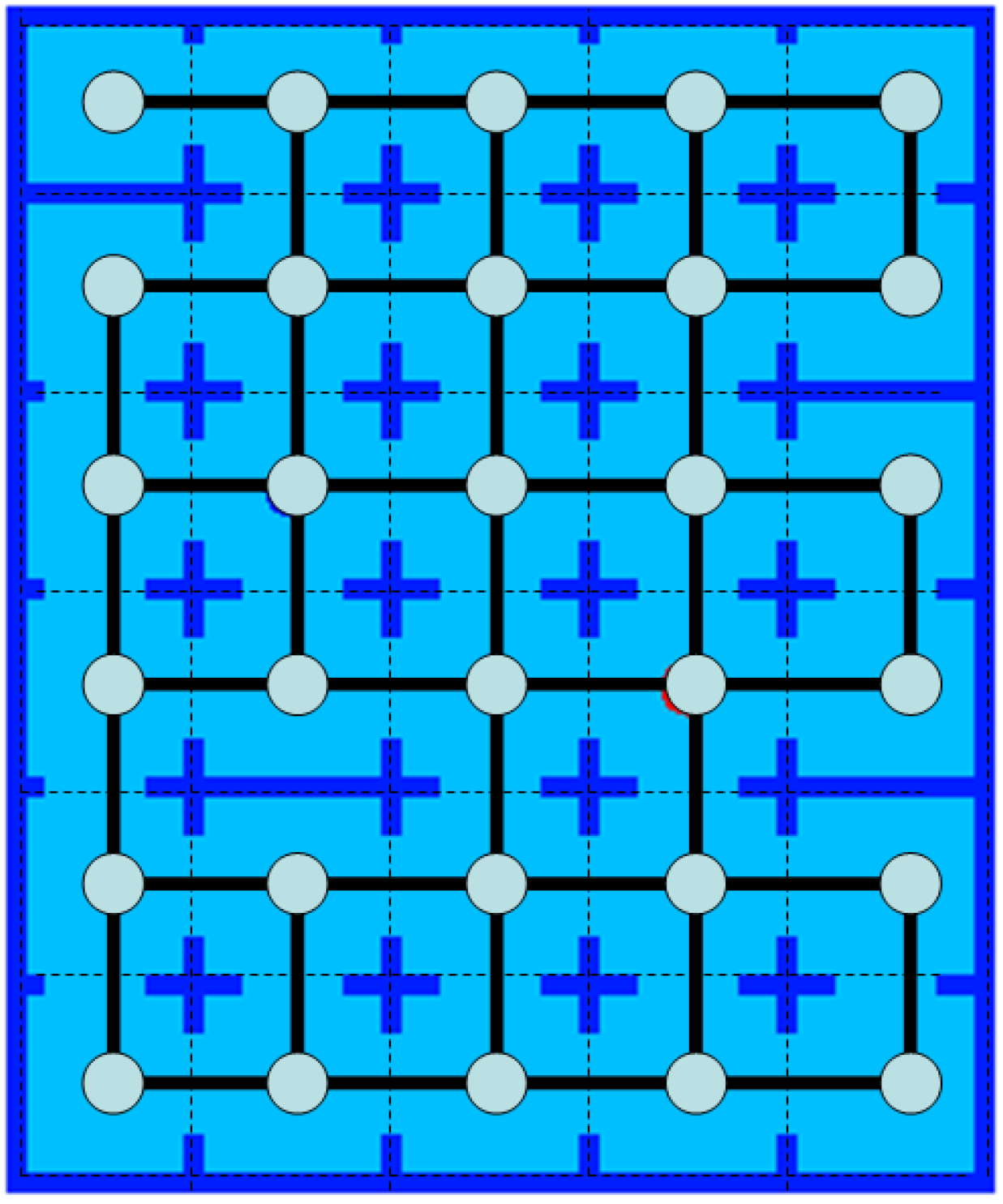
3.5. The Edge CR Games

As already mentioned, every edge CR variant can be reduced to the corresponding node variant played on L G , the line graph of G. Hence all the results and definitions of Section 3.1, Section 3.2, Section 3.3 and Section 3.4 hold for the edge variants as well. In particular, we have an edge cop number c ¯ G = c L G and capture times
c t ¯ G = c t L G , d c t ¯ G = d c t L G , c t ¯ i G = c t i L G , d c t ¯ i G = d c t i L G
In general, all of these “edge CR parameters” will differ from the corresponding “node CR parameters”.

4. The Cost of Visibility

4.1. Cost of Visibility in the Node CR Games

As already remarked, we expect that ai-CR is more difficult (from C’s point of view) than av-CR (the same holds for the drunk counterparts of this game). We quantify this statement by introducing the cost of visibility (COV).
Definition 8. For every G, the adversarial cost of visibility is H a ( G ) = c t i ( G ) c t ( G ) and the drunk cost of visibility is H d ( G ) = d c t i ( G ) d c t ( G ) .
Clearly, for every G we have H a G 1 and H d G 1 (i.e., it is at least as hard to capture an invisible robber than a visible one). The following theorem shows that in fact both H a G and H d G can become arbitrarily large. In proving the corresponding theorems, we will need the family of long star graphs S N , M . For specific values of M and N, S N , M consists of N paths (we call these rays) each having M nodes, joined at a central node, as shown in Figure 1.
Figure 1. (a): the star graph S N , 1 ; (b): the long star graph S N , M .
Robotics 03 00371 g001
Theorem 8. For every N N we have H a S N , 1 = N .
Proof. (i)   Computing   ct S N , 1 ¯ . In av-CR, for every N N we have ct S N , 1 = 1 : the cop starts at X 0 = 0 , the robber starts at some Y 0 = u 0 and, at t = 1 , he is captured by the cop moving into u ; i.e., ct S N , 1 1 ; on the other hand, since there are at least two vertices ( N 1 ), clearly ct S N , 1 1 .
(ii)   Computing   ct i S N , 1 ¯ . Let us now show that in ai-CR we have ct i S N , 1 = N . C places the cop at X 0 = 0 and R places the robber at some Y 0 = u 0 . We will obtain ct i S N , 1 by bounding it from above and below. For an upper bound, consider the following C strategy. Since C does not know the robber’s location, he must check the leaf nodes one by one. So at every odd t he moves the cop into some u 1 , 2 , , N and at every even t he returns to 0. Note that R cannot change the robber’s original position; in order to do this, the robber must pass through 0 but then he will be captured by the cop (who either is already in 0 or will be moved into it just after the robber’s move). Hence C can choose the nodes he will check on odd turns with uniform probability and without repetitions. Equivalently, we can assume that the order in which nodes are chosen by C is selected uniformly at random from the set of all permutations; further, we assume that R (who does not know this order) starts at some Y 0 = u 1 , , N . Then we have
ct i S N , 1 1 N · 1 + 1 N · 3 + + 1 N · 2 N 1 = N
For a lower bound, consider the following R strategy. The robber is initially placed at a random leaf that is different than the one selected by C (if the cop did not start at the center). Knowing this, the best C strategy is to check (in any order) all leaves without repetition. If the cop starts at the center, we get exactly the same sum as for the upper bound. Otherwise, we have
ct i S N , 1 1 N 1 · 2 + 1 N 1 · 4 + + 1 N 1 · 2 N 2 = N
(iii)   Computing   H a S N , 1 ¯ . Hence, for all N N we have H a S N , 1 = ct i S N , 1 ct S N , 1 = N  ☐
Theorem 9. For every N N { 1 } we have
H d S N , M = ( 1 + o ( 1 ) ) ( 2 N 1 ) ( N 1 ) + 1 N 2 N 3
where the asymptotics is with respect to M; N is considered a fixed constant.
Proof. (i)   Computing   dct S N , M ¯ . We will first show that, for any N N , we have dct S N , M = 1 + o 1 M 2 (recall that the parameter N is a fixed constant whereas M .) Suppose that the cop starts on the i -th ray, at distance ( 1 + o ( 1 ) ) cM from the center (for some constant c [ 0 , 1 ] ). The robber starts at a random vertex. It follows that for any j such that 1 j N , the robber starts on the j -th ray with probability ( 1 + o ( 1 ) ) / N . It is a straightforward application of Chernoff bounds to show that with probability 1 + o ( 1 ) the robber will not move by more than o ( M ) in the next O ( MN ) = O ( M ) steps, which suffice to finish the game. This is so because, if X has a binomial distribution Bin ( n , p ) , then Pr ( | X np | ϵ np ) 2 exp ( ϵ 2 np / 3 ) for any ϵ 3 / 2 . Now suppose the robber starts at distance ω ( M 2 / 3 ) from the center. During N = O ( M ) steps the robber makes in expectation N / 2 steps towards the center, and N / 2 steps towards the end of the ray. The probability to make during N steps more than N / 2 + M 2 / 3 steps towards the center, say, is thus at most e cM 1 / 3 , and the same holds also by taking a union bound over all O ( M ) steps. Hence, with probability at least 1 e cM 1 / 3 he will throughout O ( M ) steps remain at distance O ( M 2 / 3 ) from his initial position. In short, the expected capture time is easy to calculate.
  • With probability ( 1 c + o ( 1 ) ) / N , the robber starts on the same ray as the cop but farther away from the center. Conditioning on this event, the expected capture time is M ( 1 c + o ( 1 ) ) / 2 .
  • With probability ( c + o ( 1 ) ) / N , the robber starts on the same ray as the cop but closer to the center. Conditioning on this event, the expected capture time is M ( c + o ( 1 ) ) / 2 .
  • With probability ( N 1 + o ( 1 ) ) / N , the robber starts on different ray than the cop. Conditioning on this event, the expected capture time is ( c + o ( 1 ) ) M + M ( 1 / 2 + o ( 1 ) ) .
It follows that the expected capture time is
( 1 + o ( 1 ) ) M 1 c N · 1 c 2 + c N · c 2 + N 1 N · 2 c + 1 2
which is maximized for c = 0 , giving dct S N , M = 1 + o 1 M 2 .
(ii)   Computing   dct i S N , M ¯ . The initial placement for the robber is the same as in the visible variant, that is, the uniform distribution is used. However, since the robber is now invisible, C has to check all rays. As before, by Chernoff bounds, with probability at least 1 e cM 1 / 3 (for some constant c > 0 ) during O ( M ) steps the robber is always within distance O ( M 2 / 3 ) from its initial position. If the robber starts at distance ω ( M 2 / 3 ) from the center, he will thus with probability at least 1 e cM 1 / 3 not change his ray during O ( M ) steps. Otherwise, he might change from one ray to the other with bigger probability, but note that this happens only with the probability of the robber starting at distance O ( M 2 / 3 ) from the center, and thus with probability at most O ( M 1 / 3 ) . Keeping these remarks in mind, let us examine “reasonable” C strategies. It turns out there exist three such.
(ii.1) Suppose C starts at the end of one ray (chosen arbitrarily), goes to the center, and then successively checks the remaining rays without repetition, with probability at least 1 O ( M 1 / 3 ) , the robber will be caught. If the robber is caught (this implies that the robber did not switch rays), the capture time is calculated as follows:
  • With probability ( 1 + o ( 1 ) ) / N , the robber starts on the same ray as the cop. Conditioning on this event, the expected capture time is ( 1 + o ( 1 ) ) M / 2 .
  • With probability ( 1 + o ( 1 ) ) / N , the robber starts on the j -th ray visited by the cop. Conditioning on this event, the expected capture time is ( 1 + o ( 1 ) ) ( M + 2 M ( j 2 ) + M / 2 ) . ( M steps are required to move from the end of the first ray to the center, 2 M steps are `wasted’ to check j 2 rays, and M / 2 steps are needed to catch the robber on the j -th ray, on expectation.)
Hence, conditioned under not switching rays, the expected capture time in this case is
( 1 + o ( 1 ) ) M N 1 2 + 1 + 1 2 + 3 + 1 2 + + 1 + 2 ( N 2 ) + 1 2 = ( 1 + o ( 1 ) ) M N 1 2 + 2 · 1 1 2 + 2 · 2 1 2 + + 2 ( N 1 ) 1 2 = ( 1 + o ( 1 ) ) M N 1 2 + 2 N 1 2 · ( N 1 ) = ( 1 + o ( 1 ) ) M 2 · ( 2 N 1 ) ( N 1 ) + 1 N
Otherwise, if the robber is not caught, C just randomly checks rays: starting from the center, C chooses a random ray, goes until the end of the ray, returns to the center, and continues like this, until the robber is caught. The expected capture time in this case is
j 1 ( 1 1 N ) j 1 1 N 2 ( j 1 ) M + M / 2 = O ( MN ) = O ( M )
Since this happens with probability O ( M 1 / 3 ) , the contribution of the case where the robber switches rays is o ( M ) , and therefore for this strategy of C , the expected capture time is
( 1 + o ( 1 ) ) M 2 · ( 2 N 1 ) ( N 1 ) + 1 N
(ii.2) Now suppose C starts at the center of the ray, rather than the end, and checks all rays from there. By the same arguments as before, the capture time is
( 1 + o ( 1 ) ) M N 1 2 + 2 + 1 2 + 4 + 1 2 + + 2 + 2 ( N 2 ) + 1 2
which is worse than in the case when starting at the end of a ray.
(ii.3) Similarly, suppose the cop starts at distance cM from the center, for some c [ 0 , 1 ] . If he first goes to the center of the ray, and then checks all rays (suppose the one he came from is the last to be checked), then the capture time is
( 1 + o ( 1 ) ) M N c 2 2 + c + 1 2 + c + 2 + 1 2 + + c + 2 ( N 2 ) + 1 2 + ( 1 c ) 2 c + 2 ( N 1 ) + 1 c 2
which is minimized for c = 1 . And if C goes first to the end of the ray, and then to the center, the capture time is
( 1 + o ( 1 ) ) M N ( ( 1 c ) 2 2 + c 2 ( 1 c ) + c 2 + 2 ( 1 c ) + c + 1 2 + + 2 ( 1 c ) + c + 2 ( N 2 ) + 1 2
which for N 2 is also minimized for c = 1 (in fact, for N = 2 the numbers are equal).
In short, the smallest capture time is achieved when C starts at the end of some ray and therefore
dct i ( S N , M ) = ( 1 + o ( 1 ) ) M 2 · ( 2 N 1 ) ( N 1 ) + 1 N
(iii)   Computing   H d S N , M ¯ . It follows that for all N N { 1 } we have
H d S N , M = dct i S N , M dct S N , M = ( 1 + o ( 1 ) ) ( 2 N 1 ) ( N 1 ) + 1 N 2 N 3
completing the proof.  ☐

4.2. Cost of Visibility in the Edge CR Games

The cost of visibility in the edge CR games is defined analogously to that of node games.
Definition 9. For every G, the edge adversarial cost of visibility is H ¯ a ( G ) = c t ¯ i ( G ) c t ¯ ( G ) and the edge drunk cost of visibility is defined as H ¯ d ( G ) = d c t ¯ i ( G ) d c t ¯ ( G ) .
Clearly, for every G we have H ¯ a G 1 and H ¯ d G 1 . The following theorems show that in fact both H ¯ a G and H ¯ d G can become arbitrarily large. To prove these theorems we will use the previously introduced star graph S N , 1 and its line graph which is the clique K N . These graphs are illustrated in Figure 2 for N = 6 .
Figure 2. (a): the star graph S 6 , 1 and (b): its line graph, the clique K 6 .
Robotics 03 00371 g002
Theorem 10. For every N N { 1 } we have H ¯ a S N , 1 = N 1 .
Proof. We have H ¯ a ( S N , 1 ) = c t ¯ i ( S N , 1 ) c t ¯ ( S N , 1 ) = c t i ( K N ) c t ( K N ) and, since N 2 , clearly c t ( K N ) = 1 . Let us now compute c t i ( K N ) .
For an upper bound on c t i ( K N ) , C might just move to a random vertex. If the robber stays still or if he moves to a vertex different from the one occupied by C, he will be caught in the next step with probability 1 / ( N 1 ) , and thus an upper bound on the capture time is N 1 .
For a lower bound, suppose that the robber always moves to a randomly chosen vertex, different from the one occupied by C, and including the one occupied by him now (that is, with probability 1 / ( N 1 ) he stands still, and after his turn, he is with probability 1 / ( N 1 ) at each vertex different from the vertex occupied by C. Hence C is forced to move, and since he has no idea where to go, the best strategy is also to move randomly, and the robber will be caught with probability 1 / ( N 1 ) , yielding a lower bound on the capture time of N 1 . Therefore
c t i K N = N 1
Hence
H ¯ a ( S N , 1 ) = c t ¯ i ( S N , 1 ) c t ¯ ( S N , 1 ) = c t i ( K N ) c t ( K N ) = N 1
Theorem 11. For every N N { 1 } we have H ¯ d S N , 1 ) = N ( N 1 ) 2 N 3 .
Proof. This is quite similar to the adversarial case. We have H ¯ d ( S N , 1 ) = d c t ¯ i ( S N , 1 ) d c t ¯ ( S N , 1 ) = d c t i ( K N ) d c t ( K N ) . Clearly we have d c t ( K N ) = 1 1 / N (with probability 1 / N the robber selects the same vertex to start with as the cop and is caught before the game actually starts; otherwise is caught in the first round).
For d c t i ( K N ) , it is clear that the strategy of constantly moving is best for the cop, as in this case there are two chances to catch the robber (either by moving towards him, or by afterwards the robber moving onto the cop). It does not matter where he moves to as long as he keeps moving, and we may thus assume that he starts at some vertex v and moves to some other vertex w in the first round, then comes back to v and oscillates like that until the end of the game. When the cop moves to another vertex, the probability that the robber is there is 1 / ( N 1 ) . If he is still not caught, the robber moves to a random place, thereby selecting the vertex occupied by the cop with probability 1 / ( N 1 ) . Hence, the probability to catch the robber in one step is 1 N 1 + ( 1 1 N 1 ) 1 N 1 = 2 N 3 ( N 1 ) 2 . Thus, this time the capture time is a geometric random variable with probability of success equal to 2 N 3 ( N 1 ) 2 . We get d c t i ( K N ) = ( N 1 ) 2 2 N 3 and so
H ¯ d ( S N , 1 ) = d c t ¯ i ( S N , 1 ) d c t ¯ ( S N , 1 ) = d c t i ( K N ) d c t ( K N ) = ( N 1 ) 2 / ( 2 N 3 ) ( N 1 ) / N = N ( N 1 ) 2 N 3
which can become arbitrarily large by appropriate choice of N. ☐

5. Algorithms for COV Computation

For graphs of relatively simple structure (e.g., paths, cycles, full trees, grids) capture times and optimal strategies can be found by analytical arguments [9,37]. For more complicated graphs, an algorithmic solution becomes necessary. In this section we present algorithms for the computation of capture time in the previously introduced node CR variants. The same algorithms can be applied to the edge variants by replacing G with L G .

5.1. Algorithms for Visible Robbers

5.1.1. Algorithm for Adversarial Robber

The av-CR capture time c t ( G ) can be computed in polynomial time. In fact, stronger results have been presented by Hahn and MacGillivray; in [31] they present an algorithm which, given K, computes for every x , y V 2 the following:
  • C x , y , the optimal game duration when the cop/robber configuration is ( x , y ) and it is C’s turn to play;
  • R x , y , the optimal game duration when the cop/robber configuration is ( x , y ) and it is R’s turn to play.
Note that, when K < c ( G ) , there exist x , y such that C x , y = R x , y = ; Hahn and MacGillivray’s algorithm computes this correctly, as well.
The av-CR capture time can be computed by c t ( G ) = min x V max y V C x , y ; the optimal search strategies σ ^ C , σ ^ R can also be easily obtained from the optimality equations, as will be seen a little later. We have presented in [37] an implementation of Hahn and MacGillivray’s algorithm, which we call CAAR (Cops Against Adversarial Robber). Below we present this, as Algorithm 1, for the case of a single cop (the generalization for more than one cop is straightforward).
The algorithm operates as follows. In lines 01-08 C 0 x , y and R 0 x , y are initialized to , except for “diagonal” positions x , y V D 2 (i.e., positions with x = y ) for which we obviously have C x , x = R x , x = 0 . Then a loop is entered (lines 10-19) in which C i x , y is computed (line 12) by letting the cop move to the position which achieves the smallest capture time (according to the currently available estimate R i 1 x , y ); R i x , y is computed similarly in line 13, looking for the largest capture time. This process is repeated until no further changes take place, at which point the algorithm exits the loop and terminates. This algorithm is a game theoretic version of value iteration [36], which we see again in Section 5.2. It has been proved in [31] that, for any graph G and any K N , CAAR always terminates and the finally obtained C , R pair satisfies the optimality equations
x , y V D 2 : C x , y = 0 ; x , y V 2 V D 2 : C x , y = 1 + min x N x R x , y
x , y V D 2 : R x , y = 0 ; x , y V 2 V D 2 : R x , y = 1 + max y N y C x , y
The optimal memoryless strategies σ C K x , y , σ R K x , y can be computed for every position ( x , y ) by letting σ C K x , y (resp. σ R K x , y ) be a node x N x (resp. y N y ) which achieves the minimum in Equation (15) (resp. maximum in Equation (16)). The capture time c t ( G ) is computed from
c t G = min x V max y V C x , y
Algorithm 1: Cops Against Adversarial Robber (CAAR)
 Input:   G = ( V , E )
 01   For All x , y V D 2
 02     C 0 x , y = 0
 03     R 0 x , y = 0
 04   EndFor
 05   For All x , y V 2 V D 2
 06     C 0 x , y =
 07     R 0 x , y =
 08   EndFor
 09    i = 1
 10   While 1 > 0
 11    For All x , y V 2 V D 2
 12      C i x , y = 1 + min x N x R i 1 x , y
 13      R i x , y = 1 + max y N y C i x , y
 14    EndFor
 15    If C i = C i 1 And R i = R i 1
 16     Break
 17    EndIf
 18     i i + 1
 19   EndWhile
 20    C = C i
 21    R = R i
 Output:   C,  R

5.1.2. Algorithm for Drunk Robber

For any given K, value iteration can be used to determine both d c t G , K and the optimal strategy σ C K x , y ; one implementation is our CADR (Cops Against Drunk Robber) algorithm [37] which is a typical value-iteration [36] MDP algorithm; alternatively, CADR can be seen as an extension of the CAAR idea to the dv-CR. Below we present this, as Algorithm 2, for the case of a single cop (the generalization for more than one cops is straightforward).
Algorithm 2: Cops Against Drunk Robber (CADR)
 Input:   G = ( V , E ) , ε
 01  For All x , y V D 2
 02    C 0 x , y = 0
 03  EndFor
 04  For All x , y V V D 2
 05    C 0 x , y =
 06  EndFor
 07  i = 1
 08  While 1 > 0
 09   For All x , y V V D 2
 10     C i x , y = 1 + min x N x y V P x , y x , y C i 1 x , y
 11   EndFor
 12   If max x , y V 2 C i x , y C i 1 x , y < ε
 13    Break
 14   EndIf
 15    i i + 1
 16  EndWhile
 17  C = C i
 Output: C
The algorithm operates as follows (again we use C x , y to denote the optimal expected game duration when the game position is x , y ). In lines 01-06 C 0 x , y is initialized to , except for “diagonal”positions x , y V D 2 . In the main loop (lines 08-16) C i x , y is computed (line 10) by letting the cop move to the position which achieves the smallest expected capture time ( P x , y x , y in line 10 indicates the transition probability from x , y to x , y ). This process is repeated until the maximum change C i x , y C i 1 x , y is smaller than the termination criterion ε, at which point the algorithm exits the loop and terminates. This is a typical value iteration MDP algorithm [36]; the convergence of such algorithms has been studied by several authors, in various degrees of generality [38,39,40]. A simple yet strong result, derived in [39], uses the concept of proper strategy: a strategy is called proper if it yields finite expected capture time. It is proved in [39] that, if a proper strategy exists for graph G, then CADR-like algorithms converge. In the case of dv-CR we know that C has a proper strategy: it is the random walking strategy s ¯ C ( K ) mentioned in Theorem 5. Hence CADR converges and in the limit, C = lim i C i satisfies the optimality equations
x , y V D 2 : C x , y = 0 ; x , y V 2 V D 2 : C x , y = 1 + min x N x P x , y x , y C x , y
The optimal memoryless strategy σ C K x , y can be computed for every position ( x , y ) by letting σ C K x , y be a node x N x (resp. y N y ) which achieves the minimum in Equation (15) (resp. maximum in Equation (16)). The capture time d c t ( G ) is computed from
d c t G = min x V C x , y

5.2. Algorithms for Invisible Robbers

5.2.1. Algorithms for Adversarial Robber

We have not been able to find an efficient algorithm for solving the ai-CR game. Several algorithms for imperfect information stochastic games could be used to this end but we have found that they are practical only for very small graphs. The problem is that for every game position (e.g., assuming one robber and one cop, for a triple ( x , y , p ) indicating cop-position, robber-position and player to move) a full two-player, one-turn sub-game must be solved; this must be done for 2 · | V | 2 positions and for sufficient iterations to achieve convergence. The computational load quickly becomes unmanageable.

5.2.2. Algorithm for Drunk Robber

In the case of the drunk invisible robber we are also using a game tree search algorithm with pruning, for which some analytical justification can be provided. We call this the Pruned Cop Search (PCS) algorithm. Before presenting the algorithm we will introduce some notation and then prove a simple fact about expected capture time. We limit ourselves to the single cop case, since the extension to more cops is straightforward.
We let x = x 0 x 1 x 2 be an infinite history of cop moves. Letting t being the current time step, the probability vector p t contains the probabilities of the robber being in node v V or in the capture state n + 1 ; more specifically: p t = p 1 t , , p v t , , p n t , p n + 1 t and p v t = Pr y t = v | x 0 x 1 x t . Hence p t depends (as expected) on the finite cop history x 0 x 1 x t . The expected capture time is denoted by C x = E ( T | x ) ; the conditioning is on the infinite cop history. The PCS algorithm works because E T | x can be approximated from a finite part of x , as explained below. We have
C x = E T | x = t = 0 t · Pr T = t | x = t = 0 Pr T > t | x
x in the conditioning is the infinite history x = x 0 x 1 x 2 . However, for every t we have
Pr T > t | x = 1 Pr T t | x = 1 Pr T t | x 0 x 1 x t
Let us define
C t x 0 x 1 x t = τ = 0 t 1 Pr T τ | x 0 x 1 x τ = τ = 0 t 1 p n + 1 τ
where p n + 1 τ is the probability that the robber is in the capture state n + 1 at time τ (the dependence on x 0 x 1 x τ is suppressed, for simplicity of notation). Then for all t we have
C t x 0 x 1 x t = C t 1 x 0 x 1 x t 1 + 1 p n + 1 t
Update Equation (19) can be computed using only the previous cost C t 1 x 0 x 1 x τ 1 and the (previously computed) probability vector p t . While C t x 0 x t C x , we hope that (at least for the “good” histories) we have
lim t C t x 0 x t = C x
This approximation works well, with C t x 0 x t approaching its limiting value when t is in the range 15 to 20.
Below we present this, as Algorithm 3, in pseudocode. We have introduced a structure S with fields S . x , S . p , S . C = C S . x . Also we denote concatenation by the & symbol, i.e., x 0 x 1 x t & v = x 0 x 1 x t v .
Algorithm 3: Pruned Cop Search (PCS)
 Input: G = ( V , E ) , x 0 , J m a x , ε
 01    t = 0
 02    S . x = x 0 , S . p = Pr ( y 0 | x 0 ) , S . C = 0
 03    S = { S }
 04    C b e s t o l d = 0
 05   While 1 > 0
 06      S ˜ =
 07     For All S S
 08       x = S . x , p = S . p , C = S . C
 09      For All v N x t
 10        x = x & v
 11        p = p · P ( v )
 12        C = Cost ( x , p , C )
 13        S . x = x , S . p = p , S . C = C
 14        S ˜ = S ˜ { S }
 15      EndFor
 16     EndFor
 17      S = Prune ( S ˜ , J m a x )
 18      [ x b e s t , C b e s t ] = Best ( S )
 19     If | C b e s t C b e s t o l d | < ε
 20      Break
 21     Else
 22       C b e s t o l d = C b e s t
 23       t t + 1
 24     EndIf
 25   EndWhile
 Output:   x b e s t , C b e s t = C x b e s t .
The PCS algorithm operates as follows. At initialization (lines 01-04), we create a single S structure (with S . x being the initial cop position, S . p the initial, uniform robber probability and S . C = 0 ) which we store in the set S . Then we enter the main loop (lines 05-25) where we pick each available cop sequence x of length t (line 08). Then, in lines 09-15 we compute, for all legal extensions x = x & v (where v N x t ) of length t + 1 (line 10), the corresponding p (line 11) and C (by the subroutine Cost at line 12). We store these quantities in S which is placed in the temporary storage set S ˜ (lines 13–14). After exhausting all possible extensions of length t + 1 , we prune the temporary set S ˜ , retaining only the J max best cop sequences (this is done in line 17 by the subroutine Prune which computes “best” in terms of smallest C x ). Finally, the subroutine Best in line 18 computes the overall smallest expected capture time C b e s t = C x b e s t . The procedure is repeated until the termination criterion | C b e s t C b e s t o l d | < ε is satisfied. As explained above, the criterion is expected to be always eventually satisfied because of Equation (20).

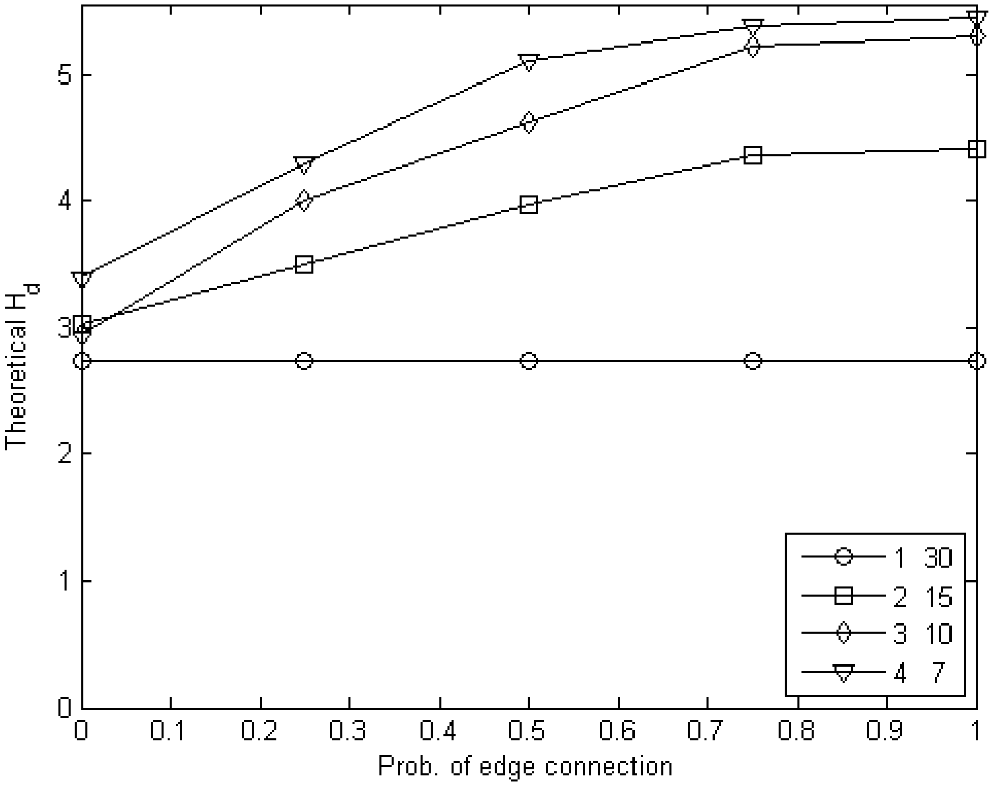
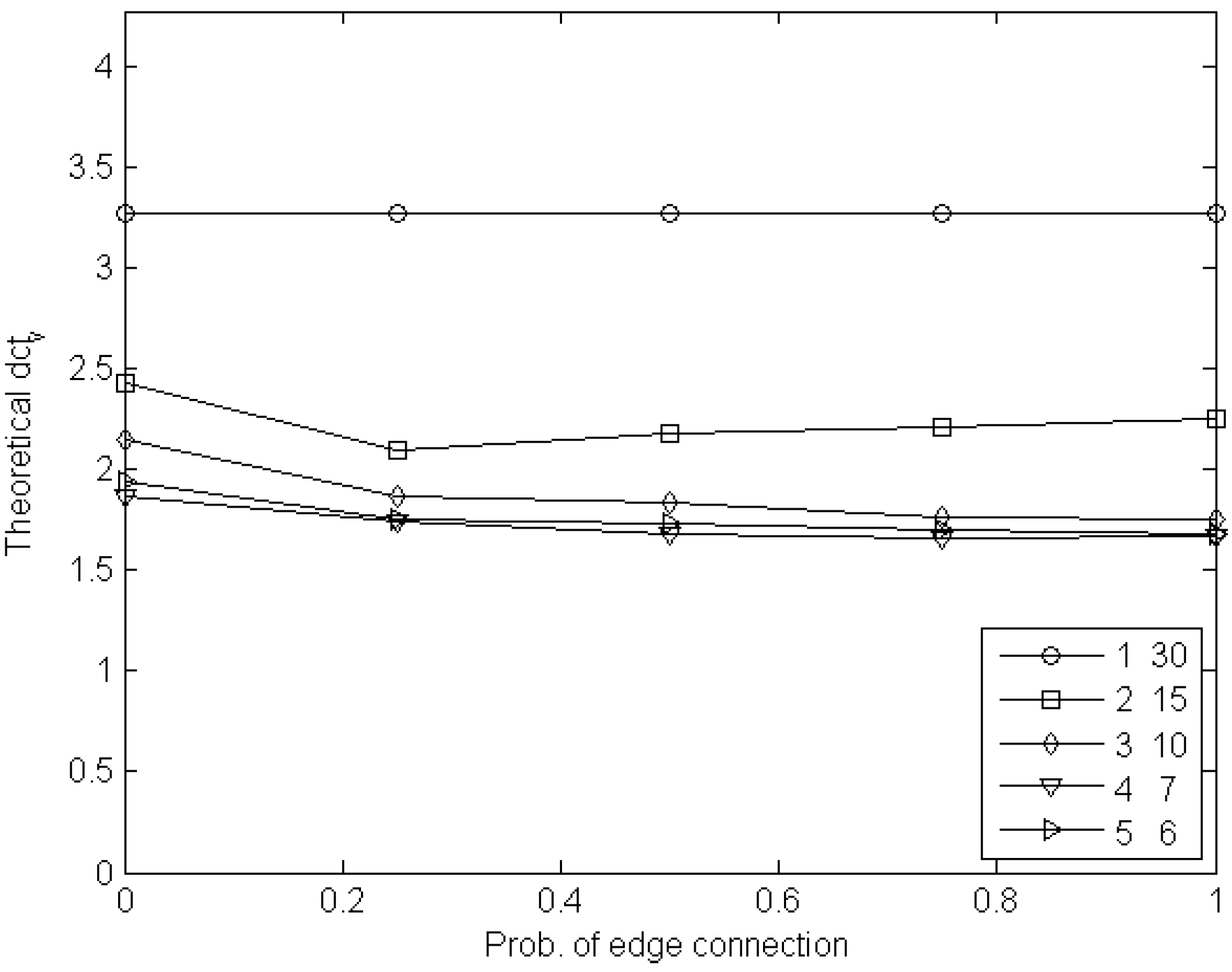
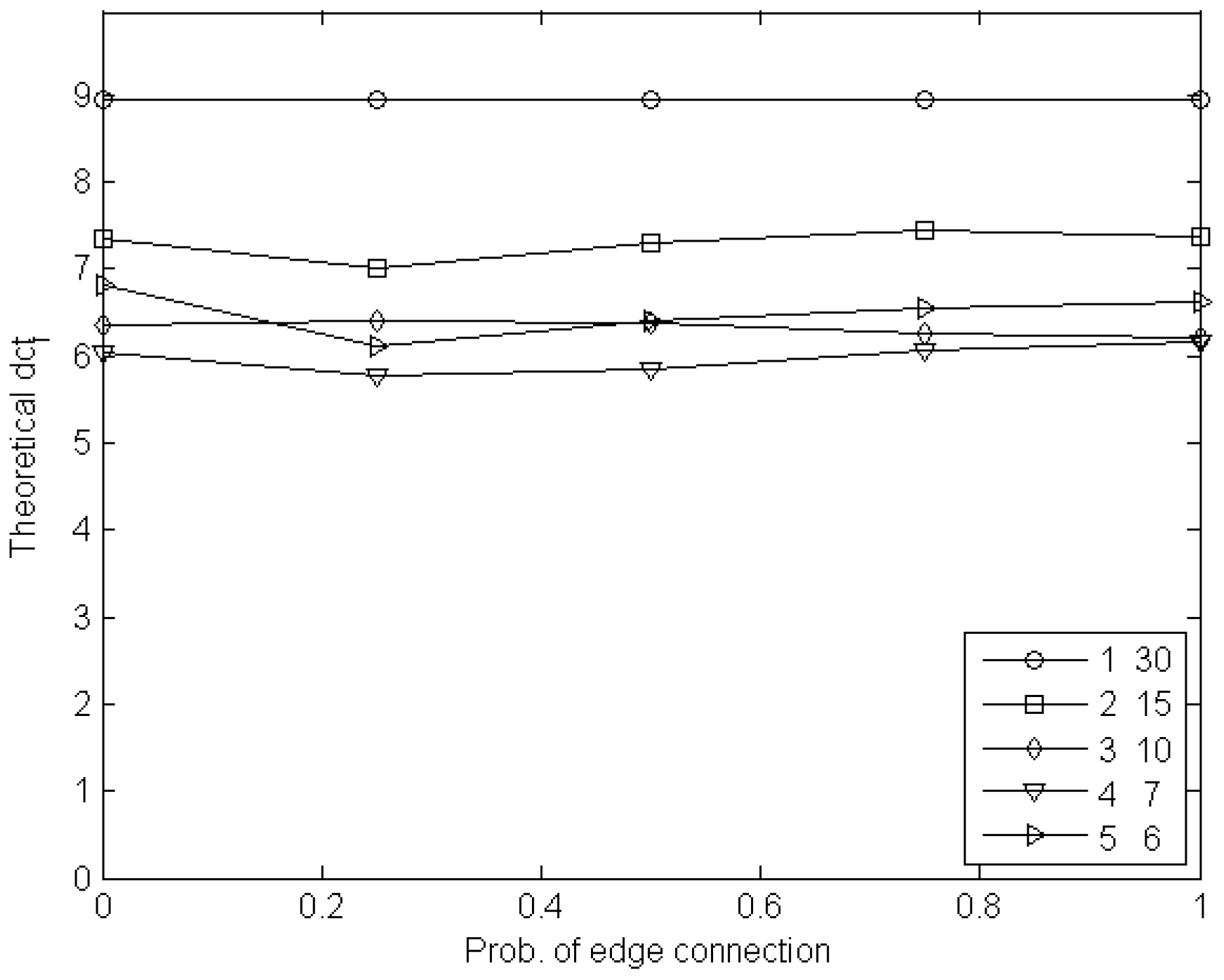
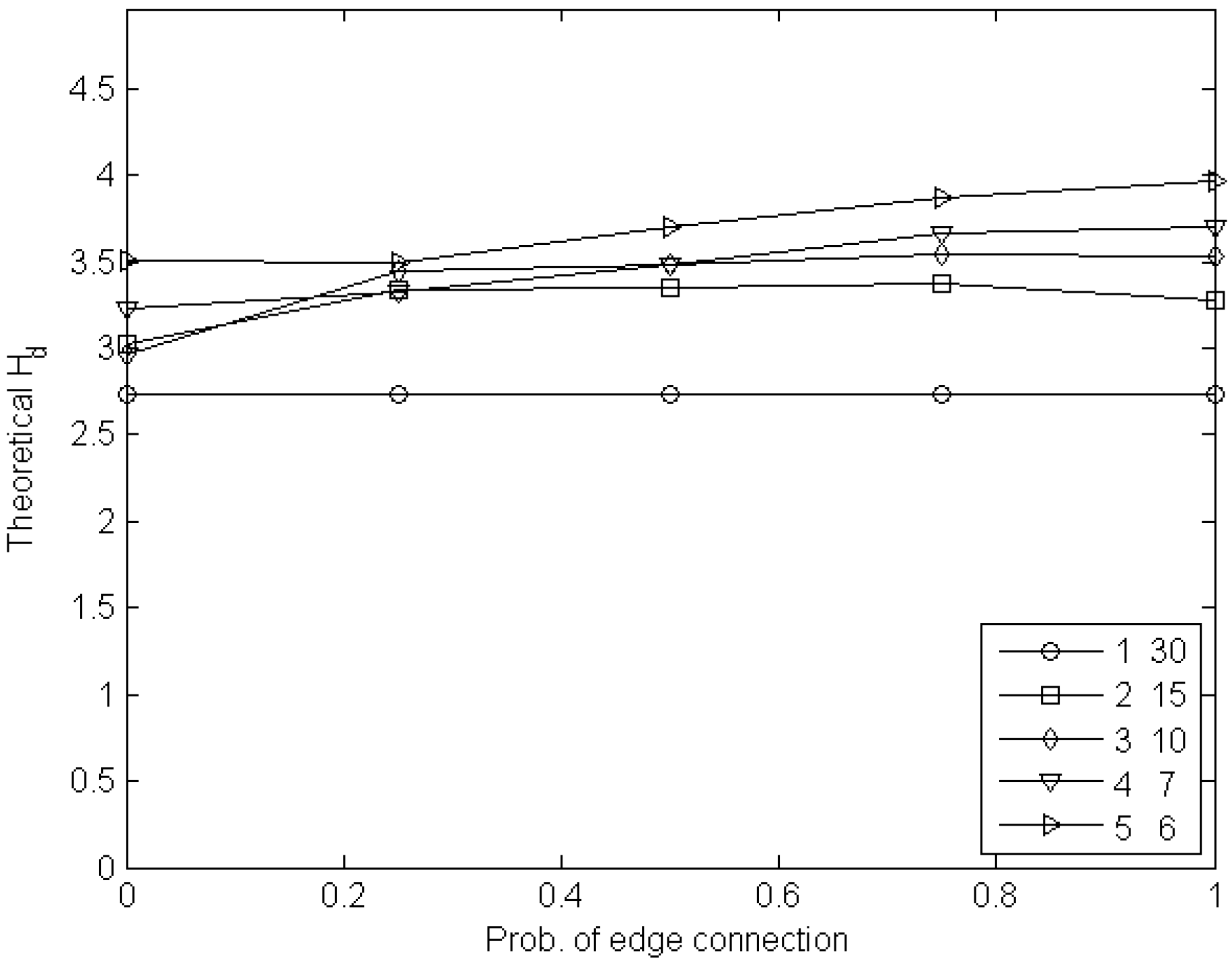
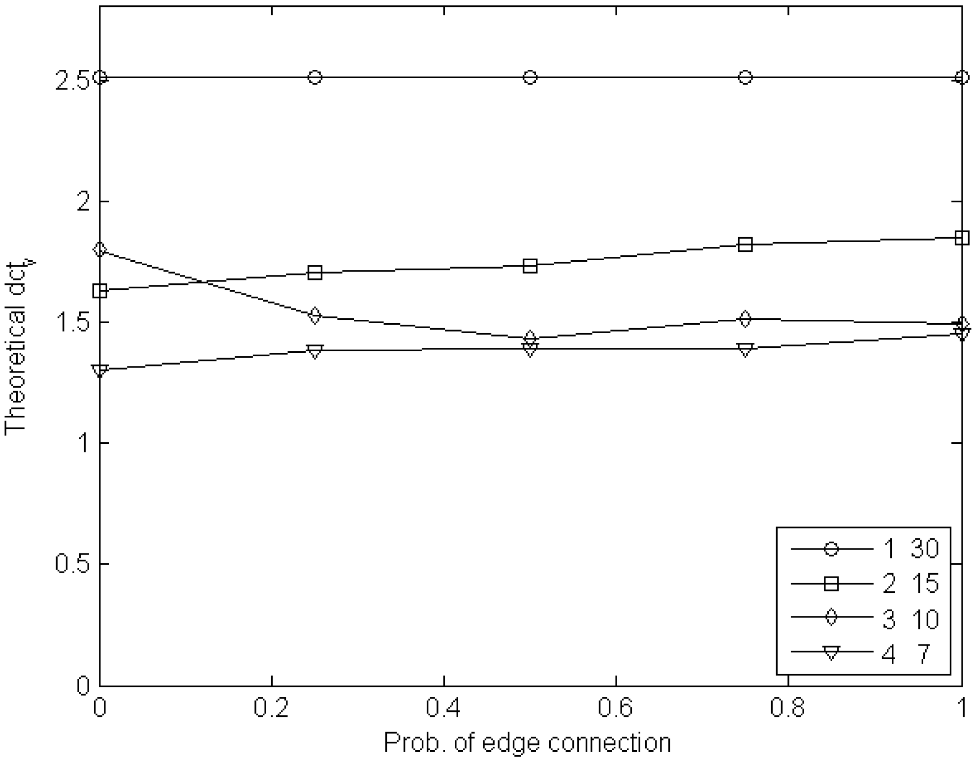
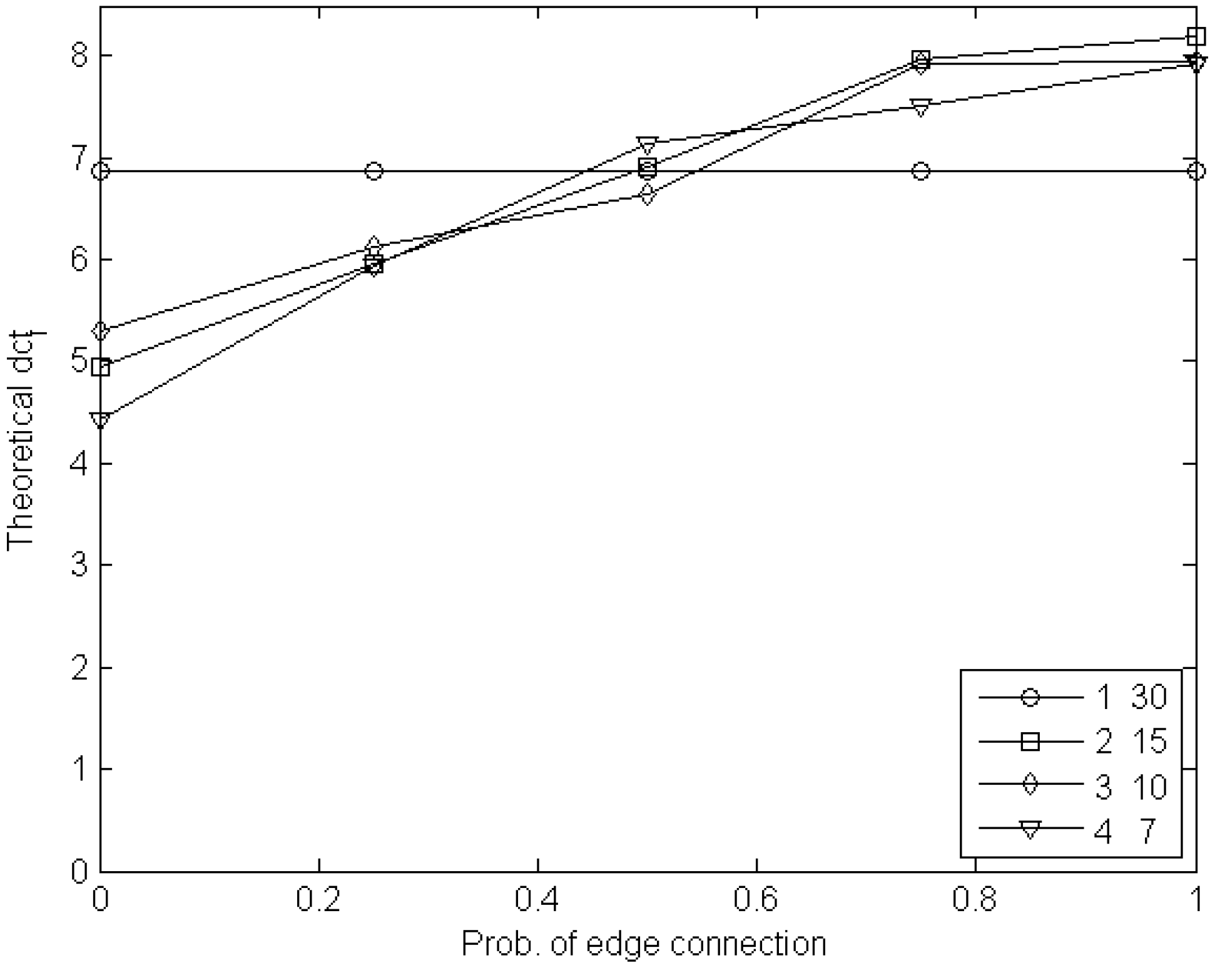
6. Experimental Estimation of the Cost of Visibility

We now present numerical computations of the drunk cost of visibility for graphs which are not amenable to analytical computation. We do not deal with the adversarial cost of visibility because, while we can compute c t G with the CAAR algorithm, we do not have an efficient algorithm to compute c t i G ; hence we cannot perform experiments on H a G = c t i G c t G . The difficulty with c t i G is that ai-CR is a stochastic game of imperfect information; even for very small graphs, one cop and one robber, ai-CR involves a state space with size far beyond the capabilities of currently available stochastic games algorithms (see [41]). In Section 6.1 we deal with node games and in Section 6.2 with edge games.

6.1. Experiments with Node Games

Since H d G = d c t i G d c t G , we use the CADR algorithm to compute d c t G and the PCS algorithm to compute d c t i G . We use graphs G obtained from indoor environments, which we represent by their floorplans. In Figure 3 we present a floorplan and its graph representation. The graph is obtained by decomposing the floorplan into convex cells, assigning each cell to a node and connecting nodes by edges whenever the corresponding cells are connected by an open space.
Figure 3. A floorplan and the corresponding graph.
Robotics 03 00371 g003
We have written a script which, given some parameters, generates random floorplans and their graphs. Every floorplan consists of a rectangle divided into orthogonal “rooms”. If each internal room were connected to its four nearest neighbors we would get an M × N grid G . However, we randomly generate a spanning tree G T of G and initially introduce doors only between rooms which are connected in G T . Our final graph G is obtained from G T by iterating over all missing edges and adding each one with probability p 0 0 , 1 . Hence each floorplan is characterized by three parameters: M, N and p 0 .
We use the following pairs of M , N values: (1,30), (2,15), (3,10), (4,7), (5,6). Four of these pairs give a total of 30 nodes and the pair ( M = 4 , N = 7 ) gives n = 28 nodes; as M / N increases, we progress from a path to a nearly square grid. For each M , N pair we use five p 0 values: 0.00, 0.25, 0.50, 0.75, 1.00; note the progression from a tree ( p 0 = 0 . 00 ) to a full grid ( p 0 = 1 . 00 ). For each triple M , N , p 0 we generate 50 floorplans, obtain their graphs and for each graph G we compute d c t ( G ) using CADR, d c t i G using PCS and H d G = d c t i G d c t G ; finally we average H d G over the 50 graphs. In Figure 4 we plot d c t ( G ) as a function of the probability p 0 ; each plotted curve corresponds to an M , N pair. Similarly, in Figure 5 we plot d c t i ( G ) and in Figure 6 we plot H d ( G ) .
Figure 4. d c t ( G ) curves for floorplans with n = 30 or n = 28 cells. Each curve corresponds to a fixed ( M , N ) pair. The horizontal axis corresponds to the edge insertion probability p 0 .
Robotics 03 00371 g004
Figure 5. d c t i ( G ) curves for floorplans with n = 30 or n = 28 cells. Each curve corresponds to a fixed ( M , N ) pair. The horizontal axis corresponds to the edge insertion probability p 0 .
Robotics 03 00371 g005
Figure 6. H d ( G ) curves for floorplans with n = 30 or n = 28 cells. Each curve corresponds to a fixed ( M , N ) pair. The horizontal axis corresponds to the edge insertion probability p 0 .
Robotics 03 00371 g006
We can see in Figure 4 and Figure 5 that both d c t G and d c t i G are usually decreasing functions of the M / N ratio. However the cost of visibility H d G increases with M / N . This is due to the fact that, when the M / N ratio is low, G is closer to a path and there is less difference in the search schedules and capture times between dv-CR and di-CR. On the other hand, for high M / N ratio, G is closer to a grid, with a significantly increased ratio of edges to nodes (as compared to the low M / N , path-like instances). This, combined with the loss of information (visibility), results in H d ( G ) being an increasing function of M / N . The increase of H d G with p 0 can be explained in the same way, since increasing p 0 implies more edges and this makes the cops’ task harder.

6.2. Experiments with Edge Games

Next we deal with H ¯ d G = d c t ¯ i G d c t ¯ G . We use graphs G obtained from mazes such as the one illustrated in Figure 7. Every corridor of the maze corresponds to an edge; corridor intersections correspond to nodes. The resulting graph G is also depicted in Figure 7. From G we obtain the line graph L ( G ) , to which we apply CADR to compute d c t L ( G ) = d c t ¯ G and PCS to compute d c t i L ( G ) = d c t ¯ i G .
Figure 7. A maze and the corresponding graph.
Robotics 03 00371 g007
We use graphs of the same type as the ones of Section 6.1 but we now focus on the edge-to-edge movements of cops and robber. Hence from every G (obtained by a specific ( M , N , p 0 ) triple) we produce the line graph L ( G ) , for which we compute H d ( L ( G ) ) using the CADR and PCS algorithms. Once again we generate 50 graphs and present average d c t ( G ) , d c t i G and H d G results in Figure 8, Figure 9 and Figure 10. These figures are rather similar to Figure 4, Figure 5 and Figure 6, except that the increase of H ¯ d G as a function of M / N is greater than that of H d G . This is due to the fact that L ( G ) has more nodes and edges than G, hence the loss of visibility makes the edge game significantly harder than the node game. There is one exception to the above remarks, namely the case ( M , N ) = ( 1 , 30 ) ; in this case both G and L ( G ) are paths and H d G is essentially equal to H ¯ d G (as can be seen by comparing Figure 6 and Figure 10).
Figure 8. d c t ¯ ( G ) curves for floorplans with n = 30 or n = 28 cells. Each curve corresponds to a fixed ( M , N ) pair. The horizontal axis corresponds to the edge insertion probability p 0 .
Robotics 03 00371 g008
Figure 9. d c t ¯ i ( G ) curves for floorplans with n = 30 or n = 28 cells. Each curve corresponds to a fixed ( M , N ) pair. The horizontal axis corresponds to the edge insertion probability p 0 .
Robotics 03 00371 g009
Figure 10. H ¯ d G curves for floorplans with n = 30 or n = 28 cells. Each curve corresponds to a fixed ( M , N ) pair. The horizontal axis corresponds to the edge insertion probability p 0 .
Robotics 03 00371 g010

7. Conclusions

In this paper we have studied two versions of the cops and robber game: the one is played on the nodes of a graph and the other played on the edges. For each version, we studied four variants, obtained by changing the visibility and adversariality assumptions regarding the robber; hence we have a total of eight CR games. For each of these we have defined rigorously the corresponding optimal capture time, using game theoretic and probabilistic tools.
Then, for the node games we have introduced the adversarial cost of visibility H G = c t i G c t G and the drunk cost of visibility H d G = d c t i G d c t G . These ratios quantify the increase in difficulty of the CR game when the cop is no longer aware of the robber’s position (this situation occurs often in mobile robotics).
We have defined analogous quantities ( H ¯ G = c t i ¯ G c t ¯ G , H ¯ d G = d c t ¯ i G d c t ¯ G ) for the edge CR games.
We have studied analytically H G and H d G and have established that both can get arbitrarily large. We have established similar results for H ¯ G and H ¯ d G . In addition, we have studied H d G and H ¯ d G by numerical experiments which support both the game theoretic results of the current paper and the analytical computations of capture times presented in [9,37].

Author Contributions

Each of the three authors of the paper has contributed to all aspects of the theoretical analysis. The numerical experiments were designed and implemented by Athanasios Kehagias.

Conflicts of Interest

The authors declare no conflict of interest.

References

  1. Chung, T.H.; Hollinger, G.A.; Isler, V. Search and pursuit-evasion in mobile robotics. Auton. Robots 2011, 31, 299–316. [Google Scholar] [CrossRef]
  2. Isler, V.; Karnad, N. The role of information in the cop-robber game. Theor. Comput. Sci. 2008, 399, 179–190. [Google Scholar] [CrossRef]
  3. Alspach, B. Searching and sweeping graphs: A brief survey. Le Matematiche 2006, 59, 5–37. [Google Scholar]
  4. Bonato, A.; Nowakowski, R. The Game of Cops and Robbers on Graphs; AMS: Providence, RI, USA, 2011. [Google Scholar]
  5. Fomin, F.V.; Thilikos, D.M. An annotated bibliography on guaranteed graph searching. Theor. Comput. Sci. 2008, 399, 236–245. [Google Scholar] [CrossRef]
  6. Nowakowski, R.; Winkler, P. Vertex-to-vertex pursuit in a graph. Discret. Math. 1983, 43, 235–239. [Google Scholar] [CrossRef]
  7. Dereniowski, D.; Dyer, D.; Tifenbach, R.M.; Yang, B. Zero-visibility cops and robber game on a graph. In Frontiers in Algorithmics and Algorithmic Aspects in Information and Management; Springer: Berlin, Germany, 2013; pp. 175–186. [Google Scholar]
  8. Isler, V.; Kannan, S.; Khanna, S. Randomized pursuit-evasion with local visibility. SIAM J. Discret. Math. 2007, 20, 26–41. [Google Scholar] [CrossRef]
  9. Kehagias, A.; Mitsche, D.; Prałat, P. Cops and invisible robbers: The cost of drunkenness. Theor. Comput. Sci. 2013, 481, 100–120. [Google Scholar] [CrossRef]
  10. Adler, M.; Racke, H.; Sivadasan, N.; Sohler, C.; Vocking, B. Randomized pursuit-evasion in graphs. Lect. Notes Comput. Sci. 2002, 2380, 901–912. [Google Scholar]
  11. Vieira, M.; Govindan, R.; Sukhatme, G.S. Scalable and practical pursuit-evasion. In Proceedings of the 2009 IEEE Second International Conference on Robot Communication and Coordination (ROBOCOMM’09), Odense, Denmark, 31 March–2 April 2009; pp. 1–6.
  12. Gerkey, B.; Thrun, S.; Gordon, G. Parallel stochastic hill-climbing with small teams. In Multi-Robot Systems. From Swarms to Intelligent Automata; Springer: Dordrecht, Netherlands, 2005; Volume III, pp. 65–77. [Google Scholar]
  13. Hollinger, G.; Singh, S.; Djugash, J.; Kehagias, A. Efficient multi-robot search for a moving target. Int. J. Robot. Res. 2009, 28, 201–219. [Google Scholar] [CrossRef]
  14. Hollinger, G.; Singh, S.; Kehagias, A. Improving the efficiency of clearing with multi-agent teams. Int. J. Robot. Res. 2010, 29, 1088–1105. [Google Scholar] [CrossRef]
  15. Lau, H.; Huang, S.; Dissanayake, G. Probabilistic search for a moving target in an indoor environment. In Proceedings of the 2006 IEEE/RSJ International Conference on Intelligent Robots and Systems, Beijing, China, 9–15 October 2006; pp. 3393–3398.
  16. Sarmiento, A.; Murrieta, R.; Hutchinson, S.A. An efficient strategy for rapidly finding an object in a polygonal world. In Proceedings of the 2003 IEEE/RSJ International Conference on Intelligent Robots and Systems(IROS 2003), Las Vegas, NV, USA, 27–31 October 2003; Volume 2, pp. 1153–1158.
  17. Hsu, D.; Lee, W.S.; Rong, N. A point-based POMDP planner for target tracking. In Proceedings of the 2008 IEEE International Conference on Robotics and Automation (ICRA 2008), Pasadena, CA, USA, 19–23 May 2008; pp. 2644–2650.
  18. Kurniawati, H.; Hsu, D.; Lee, W.S. Sarsop: Efficient point-based POMDP planning by approximating optimally reachable belief spaces. In Proceedings of Robotics: Science and Systems, Zurich, Switzerland, 25–28 June 2008.
  19. Pineau, J.; Gordon, G. POMDP planning for robust robot control. Robot. Res. 2007, 28, 69–82. [Google Scholar]
  20. Smith, T.; Simmons, R. Heuristic search value iteration for POMDPs. In Proceedings of the 20th Conference on Uncertainty in Artificial Intelligence, Banff, Canada, 7–11 July 2004; pp. 520–527.
  21. Spaan, M.T.J.; Vlassis, N. Perseus: Randomized point-based value iteration for POMDPs. J. Artif. Intel. Res. 2005, 24, 195–220. [Google Scholar]
  22. Hauskrecht, M. Value-function approximations for partially observable Markov decision processes. J. Artif. Intel. Res. 2000, 13, 33–94. [Google Scholar]
  23. Littman, M.L.; Cassandra, A.R.; Kaelbling, L.P. Efficient Dynamic-Programming Updates in Partially Observable Markov Decision Processes; Technical Report CS-95-19; Brown University: Providence, RI, USA, 1996. [Google Scholar]
  24. Monahan, G.E. A survey of partially observable Markov decision processes: Theory, models, and algorithms. Manag. Sci. 1982, 28, 1–16. [Google Scholar] [CrossRef]
  25. Canepa, D.; Potop-Butucaru, M.G. Stabilizing Flocking Via Leader Election in Robot Networks. In Proceedings of the 9th International Symposium on Stabilization, Safety, and Security of Distributed Systems (SSS 2007), Paris, France, 14–16 November 2007; pp. 52–66.
  26. Gervasi, V.; Prencipe, G. Robotic Cops: The Intruder Problem. In Proceedings of the 2003 IEEE Conference on Systems, Man and Cybernetics (SMC 2003), Washington, DC, USA, 5–8 October 2003; pp. 2284–2289.
  27. Prencipe, G. The effect of synchronicity on the behavior of autonomous mobile robots. Theory Comput. Syst. 2005, 38, 539–558. [Google Scholar] [CrossRef]
  28. Dudek, A.; Gordinowicz, P.; Pralat, P. Cops and robbers playing on edges. J. Comb. 2013, 5, 131–153. [Google Scholar] [CrossRef]
  29. Kuhn, H.W. Extensive games. Proc. Natl. Acad. Sci. USA 1950, 36, 570–576. [Google Scholar] [CrossRef] [PubMed]
  30. Bonato, A.Y.; Macgillivray, G. A General Framework for Discrete-Time Pursuit Games, preprint.
  31. Hahn, G.; MacGillivray, G. A note on k-cop, l-robber games on graphs. Discret. Math. 2006, 306, 2492–2497. [Google Scholar] [CrossRef]
  32. Berwanger, D. Graph Games with Perfect Information, preprint.
  33. Mazala, R. Infinite games. Automata, Logics and Infinite Games 2002, 2500, 23–38. [Google Scholar]
  34. Aigner, M.; Fromme, M. A game of cops and robbers. Discret. App. Math. 1984, 8, 1–12. [Google Scholar] [CrossRef]
  35. Osborne, M.J. A Course in Game Theory; MIT Press: Cambridge, MA, USA, 1994. [Google Scholar]
  36. Puterman, M.L. Markov Decision Processes: Discrete Stochastic Dynamic Programming; John Wiley & Sons, Inc.: New York, NY, USA, 1994. [Google Scholar]
  37. Kehagias, A.; Prałat, P. Some remarks on cops and drunk robbers. Theor. Comput. Sci. 2012, 463, 133–147. [Google Scholar] [CrossRef]
  38. De la Barrière, R.P. Optimal Control Theory: A Course in Automatic Control Theory; Dover Pubns: New York, NY, USA, 1980. [Google Scholar]
  39. Eaton, J.H.; Zadeh, L.A. Optimal pursuit strategies in discrete-state probabilistic systems. Trans. ASME Ser. D J. Basic Eng. 1962, 84, 23–29. [Google Scholar] [CrossRef]
  40. Howard, R.A. Dynamic Probabilistic Systems, Volume Ii: Semi-Markov and Decision Processes; Dover Publications: New York, NY, USA, 1971. [Google Scholar]
  41. Raghavan, T.E.S.; Filar, J.A. Algorithms for stochastic games—A survey. Math. Methods Oper. Res. 1991, 35, 437–472. [Google Scholar] [CrossRef]

